Article

NCD-Pred: Forecasting Multichannel Shipboard Electrical Power Demand Using Neighborhood-Constrained VMD

1
Institute of Marine Engineering (INM), National Research Council (CNR), 90153 Palermo, Italy
2
Institute of Complex Systems (ISC), National Research Council (CNR), 00185 Rome, Italy
3
Institute of Marine Engineering (INM), National Research Council (CNR), 00128 Rome, Italy
*
Author to whom correspondence should be addressed.
Forecasting 2025, 7(3), 44; https://doi.org/10.3390/forecast7030044
Submission received: 25 June 2025 / Revised: 8 August 2025 / Accepted: 11 August 2025 / Published: 13 August 2025
(This article belongs to the Special Issue Feature Papers of Forecasting 2025)

Abstract

This paper introduces Neighborhood-Constrained Decomposition-based Prediction (NCD-Pred), the first system to leverage Neighborhood-Constrained Variational Mode Decomposition (NCVMD) for multichannel forecasting by integrating time series decomposition and neural networks. NCD-Pred leverages NCVMD to decompose a multichannel signal into simpler, band-limited components—referred to as intrinsic mode functions or simply modes—by prioritizing the most informative channel (the main channel) over less informative ones (the auxiliary channels) and bringing their central frequencies into alignment up to a tunable extent. This frequency synchronization provides a framework for cooperative mode forecasting, where predictions of signal components are recombined to produce the original signal prediction. For mode-level forecasting, Long Short-Term Memory (LSTM) networks are utilized. NCD-Pred’s performance is evaluated against similarly designed mode-level forecasting systems using a multichannel dataset with weak cross-correlation, representing power load on a large vessel. The results show that NCD-Pred outperforms benchmark methods, demonstrating its practical utility in real signal processing scenarios.

1. Introduction

Time series forecasting has become an essential methodology across a wide range of domains, including energy systems, environmental monitoring, transportation, finance, and beyond. As operational environments grow increasingly complex, traditional single-channel forecasting (often also referred to as univariate in stochastic process terminology) approaches (as specified in Section 2.1, in this work, multi-channel forecasting—often termed multivariate in stochastic process terminology—refers to forecasting from multi-channel input, while the actual forecast focuses on only one channel) have given way to methods capable of capturing intricate interdependencies among multiple variables. This evolution reflects the fundamental challenge of modeling real-world systems where single-variable analysis often proves insufficient for accurate predictions.
In recent years, data-driven forecasting models leveraging machine learning (ML) and deep learning (DL) methodologies have demonstrated exceptional performance, particularly in hybrid architectures. These hybrid models, also known as cooperative ensemble approaches, execute forecasting through sequential subtasks including data preprocessing, hyperparameter optimization, feature selection, and post-processing procedures [1]. The integration of decomposition techniques with neural predictors has proven especially effective for addressing the non-linear and non-stationary characteristics inherent in complex time series data.
Among decomposition methods, Variational Mode Decomposition (VMD) [2] has gained significant traction due to its superior robustness to sampling rate and noise compared to earlier techniques such as Empirical Mode Decomposition (EMD) [3]. The VMD approach enables the extraction of intrinsic mode functions (IMFs) that effectively capture underlying patterns across different frequency bands, providing valuable preprocessing capabilities for subsequent forecasting algorithms. These IMFs represent “well-behaved” sub-signals that are more regular and predictable than the original complex signal, making the forecasting task considerably more manageable.

1.1. Related Work

The efficacy of VMD-based hybrid approaches for single-channel forecasting has been demonstrated across diverse applications. For electric load forecasting, numerous studies have employed VMD as a preprocessing step prior to neural network prediction. Haykal et al. [4] developed a hybrid model combining VMD with Multi-Layer Perceptron (MLP) Artificial Neural Networks for household electricity consumption forecasting, achieving superior accuracy compared to classical autoregressive moving average models. Similarly, Chao et al. [5] utilized VMD for signal feature extraction coupled with an attention-enhanced Long Short-Term Memory (LSTM) network for short-term power load forecasting.
More sophisticated architectures have further advanced single-channel forecasting capabilities. Huang et al. [6] proposed an electric load forecasting model integrating VMD preprocessing with a deep, bidirectional LSTM network enhanced by attention mechanisms, employing particle swarm optimization (PSO) for hyperparameter tuning to address highly nonlinear and volatile load sequences. In a similar vein Fazzini et al. [7] implemented VMD as a preprocessing stage for LSTM-based forecasting to predict electric load demand on large passenger ships through mode-level prediction over multiple time steps.
Zhou et al. [8], Zhang et al. [9], and Xiong et al. [10] utilized VMD to preprocess electrical load data before executing short-term predictions with hybrid models incorporating Time Convolutional Networks (TCNs) and various enhancement strategies. Zhang et al. [11] combined VMD decomposition with self-recurrent mechanisms and Vector Support Regression models optimized via the Cuckoo Search algorithm for electrical load forecasting. The versatility of these hybrid approaches has been further demonstrated in forecasting electricity production from renewable sources [12,13,14], magnetotelluric phenomena [15], and network traffic [16].
The application of VMD to forecasting is limited to single-channel time series, as VMD lacks a criterion for grouping modes generated from different channels to enable information sharing. While single-channel forecasting provides valuable insights for many applications, multi-channel forecasting offers a more comprehensive framework for systems characterized by interdependent variables. Multi-channel approaches capture relationships among concurrent data streams, enabling more nuanced predictions by leveraging cross-channel correlations and temporal dynamics. This advancement represents a natural progression in forecasting methodology, addressing the limitations of single-channel techniques when applied to complex systems. Two key heuristics have emerged as particularly important in multi-channel forecasting: (1) the primary channel to be forecasted (main channel) is the most critical, while others serve as auxiliary sources of contextual information; (2) mode decomposition facilitates forecasting by allowing each band-limited mode to be predicted separately rather than tackling a complex channel in its entirety.
Recent innovations in forecasting from multi-channel input have yielded remarkable results across diverse domains. Wang et al. [17] introduced a novel air quality index (AQI) forecasting paradigm that combines ternary interval-valued time series, multivariate VMD (MVMD) [18], multivariate relevance vector machine, and mixed coding particle swarm optimization. This approach uniquely captures both trend and volatility patterns in AQI by simultaneously modeling daily minimum, mean, and maximum values, demonstrating the advantage of multi-channel analysis for environmental monitoring.
In the energy sector, Huang et al. [19] developed a hybrid forecasting model integrating multivariate empirical mode decomposition (MEMD) [20], support vector regression, and particle swarm optimization for day-ahead electricity peak load prediction. The key innovation of this approach lies in applying MEMD to effectively extract inherent information from multi-channel data across different time frequencies, showcasing the value of multi-channel decomposition for energy forecasting applications.
For short-term power load forecasting, sophisticated hybrid architectures have shown promising results. Huang et al. [6] presented a deep, bidirectional LSTM network enhanced by VMD and attention mechanisms, where VMD decomposition parameters were determined by residual energy ratios and multiple BiLSTM layers captured time-series information at various scales. Building on this approach, Xiong et al. [10] proposed an integrated model combining VMD, deep temporal convolutional networks, self-attention mechanisms, and LSTM networks that decomposes load data into intrinsic components while extracting both short- and long-term temporal features with dynamic feature weight adjustment.
Beyond energy applications, Wang et al. [17] demonstrated the versatility of multi-channel forecasting in financial domains through a multiscale methodology combining MVMD with various machine learning algorithms for predicting ship prices in the volatile shipping market. This approach effectively captures complex relationships among newbuilding, secondhand, and scrap vessel prices by extracting frequency-aligned oscillatory modes, with empirical validation on Capesize bulker and Very Large Crude Carrier tanker data.
The evolution from single-channel to multi-channel forecasting reflects the growing recognition that complex systems require holistic modeling approaches capable of capturing interdependencies among multiple variables. By integrating advanced decomposition techniques like VMD and MVMD with sophisticated machine learning architectures, researchers have developed increasingly accurate forecasting methodologies applicable across diverse domains including energy systems, environmental monitoring, transportation, and finance.
The maritime sector presents a particularly compelling case for advanced forecasting techniques. With shipping accounting for approximately 3% of global greenhouse gas emissions [21] and maritime trade projected to grow by 40% over the next three decades [22], the International Maritime Organization has implemented mandatory efficiency regulations aimed at achieving net-zero emissions by 2050 [23]. Shipboard Energy Management Systems (EMSs) have emerged as a promising operational measure, with potential to reduce ships’ carbon intensity by up to 10% [24]. Accurate forecasting of electrical load demand, especially in the day-ahead horizon, is crucial for effective EMSs in maritime applications, where fluctuating sea conditions, propulsion loads, and the potential communication failures can introduce significant uncertainties in power system management [25,26].

1.2. Contribution

In this paper, we introduce a novel approach, Neighborhood-Constrained Decomposition-based Prediction (NCD-Pred), for time series prediction and apply it to shipboard electrical power demand forecasting. This method utilizes Long Short-Term Memory (LSTM) networks to predict multi-channel input time series, which are first decomposed using the recently developed Neighborhood Constraint Variational Mode Decomposition (NCVMD) technique [27]. This method naturally aligns, up to a certain tuneable limit, the central frequencies of the modes within a multichannel input, allowing the modes to work cooperatively for forecasting while maintaining the integrity of the main signal.
As thoroughly illustrated in [18], MVMD demonstrates the benefits of generating modes with similar frequency content across channels, providing a criterion for grouping modes together to enable multi-channel processing. However, enforcing strict central frequency alignment may compromise decomposition accuracy across all channels indiscriminately. A more flexible approach, such as that offered by NCVMD [27], preserves the integrity of a primary information source (main channel) while allowing a tunable trade-off between frequency alignment and decomposition error in auxiliary channels, making it better suited to a wider range of applications.
The proposed hybrid forecasting method was tested on a sample of electric power demand time series collected from a real-world large passenger ship. The results show that while preserving a pure VMD-based decomposition for the main channel, NCVMD maintains acceptable reconstruction errors for auxiliary signals while successfully enforcing modes’ frequency alignment between channels, demonstrating its practical utility in complex signal processing scenarios.
NCD-Pred introduces a novel approach that leverages NCVMD to perform forecasting from multi-channel inputs without relying on restrictive assumptions about the data structure, opening new possibilities for applying NCVMD in multi-channel time series forecasting. Furthermore, NCD-Pred contributes to the field by aligning with the ongoing trend of developing optimized decomposition methods within predictive modeling, with the goal of enhancing energy efficiency and the management of electrical power grids.
The rest of this article is structured in the following way: In Section 2 we illustrate the proposed method; specifically, we set up the forecasting nomenclature including definitions of time series, mathematical formulations of forecasting, multi-step forecasting explanations, and definitions of intrinsic mode functions (IMFs). Next, we illustrate the Neighborhood-Constrained Variational Mode Decomposition (NCVMD) methodology, including background and motivation, core principles and formulation, update rules and implementation, and applications to multi-channel forecasting and ANN-based forecasting. In Section 2.3 we describe the case study and analysis setup, detailing the ship electrical system, data collection, variable selection, test scenario design, and parameter settings. In Section 3 we present the results in terms of decomposition in the frequency domain and forecasting results. Finally, in Section 4, we provide a final discussion summarizing the NCD-Pred methodology, key findings, and suggestions for future research.

2. Materials and Methods

2.1. Forecasting Nomenclature

The relevant nomenclature used in this work is summarized in this sub-section for the sake of clarity. A time series is a set of data points indexed by time, usually taken at regular time intervals. Formally it is defined as:
{ x i } i = 1 T , x i = ( x i 1 , , x i N ) R N
where i is the time step index, T is the length of the time series, and N is the number of variables composing the time series. If N = 1 , the time series is single-channel; otherwise, it is multi-channel. Electrical power demand time series consist of active power demand measurements of one or more electrical loads.
In this work, forecasting means predicting the next value of the time series x i + 1 given the previous observations ( x 1 , , x i ) . Regardless of the value of N (whether N = 1 or N > 1 ), the forecasting task always involves predicting only one channel (or component) of x i , e.g.,  x i + 1 j , j [ 1 , N ] . Furthermore, it is often required to forecast the series for a horizon h in the future ( x i + 1 j , , x i + h j ) , a task known as multi-step forecasting.
The intrinsic mode functions (IMFs) resulting from NCVMD decomposition will also be referred to as sub-signals or simply as modes [27].

2.2. Neighborhood-Constrained Variational Mode Decomposition (Outline)

In this section, we illustrate Neighborhood-Constrained Variational Mode Decomposition (NCVMD) [27], which serves as a preprocessing step for NCD-Pred. NCVMD addresses limitations in existing decomposition methods while offering significant advantages for multi-channel forecasting applications.

2.2.1. Background and Motivation

Traditional decomposition methods like Variational Mode Decomposition (VMD) [2] and its multi-channel extension Multivariate Variational Mode Decomposition (MVMD) [18] and Variational Mode Decomposition with Mode Selection (VMDMS) [28] have proven effective for signal processing and forecasting applications. However, each presents specific limitations when applied to complex forecasting tasks.
VMD decomposes a real-valued signal f ( t ) into discrete mode functions u k ( t ) with specific sparsity properties, formulated as a constrained variational problem:
min { u k } , { ω k } k = 1 K t δ ( t ) + j π t u k ( t ) e j ω k t 2 2
subject to the constraint k = 1 K u k = f . While effective for single-channel applications, VMD lacks the ability to capture correlations across multiple channels.
MVMD addresses this limitation by extending the VMD framework to handle multi-channel signals, decomposing a C-channel signal x ( t ) = [ x 1 ( t ) , x 2 ( t ) , , x C ( t ) ] into K modes u k ( t ) = [ u k 1 ( t ) , u k 2 ( t ) , , u k C ( t ) ] . The key innovation in MVMD is its ability to align frequency across channels, enforcing a single central frequency component for each mode across all channels. This approach provides a criterion for grouping modes from different channels, enabling them to work cooperatively.
However, MVMD’s strict frequency alignment requirement presents challenges for forecasting applications where components of multi-channel data are heterogeneous variables or do not share frequency spectrum similarities, despite being homogeneous. Moreover, decomposition error issues may occur when a certain channel contains primary information, while others serve only contextual roles since MVMD treats all channels uniformly and lacks a mechanism to distribute the decomposition error in a way that preserves the primary source of information.
VMDMS introduces a criterion that enables VMD modes from different channels to work cooperatively. This criterion is based on the proximity of the modes’ central frequencies to the central frequency of the channel mode being forecasted. Proximity is controlled by a threshold, which excludes all signal modes whose central frequency distance from the main central frequency exceeds this value. Although this method shows promising results compared to VMD [28], it lacks a mechanism to actively bring the central frequencies closer together. In scenarios where a small number of modes is selected and all central frequencies exceed the threshold, the method falls back to single-channel VMD.

2.2.2. NCVMD: Core Principles and Formulation

NCVMD [27] addresses these challenges through two key heuristic principles:
  • In a multi-channel forecasting system, the main channel—which contains the primary source of information—should be treated differently from the auxiliary channels, which convey less relevant information.
  • Adjustable frequency matching among modes with closely related, yet distinct, spectral content should be supported. This enables a balance between decomposition error and alignment precision, resulting in a more flexible and adaptable algorithm.
Unlike MVMD, which enforces strict frequency alignment, NCVMD allows the main channel to be decomposed using the same constraints adopted by standard VMD, while the central frequencies of auxiliary channels’ modes are constrained to neighborhoods around those of the main channel’s modes. This approach provides a flexible framework for multi-channel forecasting, image merging, and signal denoising.
The NCVMD Lagrangian underlying the decomposition procedure [27] incorporates a neighborhood constraint term:
L u k , ω k , λ : = α k t δ ( t ) + j π t u k ( t ) e j ω k t 2 2 + f ( t ) k u k ( t ) 2 2 + λ ( t ) , f ( t ) k u k ( t ) + 2 β k ω k ω ˜ k 2 u k ( t ) 2 2 .
The first term captures variation, whereas the second and third terms correspond to reconstruction fidelity, consistent with VMD. The fourth term introduces a neighborhood constraint as defined in [27], where
  • β acts as a customizable weight that determines the influence of the neighborhood constraint;
  • ω ˜ k denotes the central frequency associated with the k-th mode of the main channel;
  • u k ( t ) 2 2 weights the influence of the frequency difference.
Weighting the central frequency difference with u k ( t ) 2 2 = u ^ ( ω ) k 2 2 naturally constrains auxiliary channel modes within low-frequency areas, accounting for the common decay pattern in real-world signals’ power spectra, where higher frequencies typically have lower energy.

2.2.3. Update Rules and Implementation

The optimization problem is recast in the frequency domain using the Parseval–Plancherel isometry under the L 2 norm. By differentiating the Lagrangian with respect to u ^ k ( ω ) and ω k , we obtain the following update rules for the iterative optimization process [27]:
u ^ k n + 1 ( ω ) = f ^ ( ω ) i k u ^ i ( ω ) + λ ^ ( ω ) 2 1 + 2 α ( ω ω k ) 2 + 2 β ( ω k ω ˜ k ) 2
ω k n + 1 = α 0 ω u ^ k ( ω ) 2 d ω + β ω ˜ k 0 u ^ k ( ω ) 2 d ω ( α + β ) 0 u ^ k ( ω ) 2 d ω
The implementation of NCVMD relies on an Alternating Direction Method of Multipliers (ADMM) approach, as outlined in Algorithm 1, where τ controls the update rate of the Lagrangian multipliers. The procedure first decomposes the main channel using VMD ( β = 0 ); the resulting central frequencies are then used as reference frequencies for decomposing the auxiliary channels ( β > 0 ).
Algorithm 1 ADMM Optimization of Neighborhood-Constrained Variational Mode Decomposition (NCVMD)
1:
Initialize:
2:
    Mode components u ^ k 1 , central frequencies ω k 1 , Lagrangian multiplier λ ^ 1 , iteration counter n 0
3:
repeat
4:
     n n + 1
5:
    Update mode components:
6:
    for  k = 1 to K do
7:
        For all ω 0 , update u ^ k using:
u ^ k n + 1 ( ω ) f ^ ( ω ) i < k u ^ i n + 1 ( ω ) i > k u ^ i n ( ω ) + λ ^ n ( ω ) 2 1 + 2 α ( ω ω k n ) 2 + 2 β ( ω k n ω ˜ k ) 2
8:
    end for
9:
    Update central frequencies:
10:
   For all k = 1 to K:
ω k n + 1 α 0 ω | u ^ k n + 1 ( ω ) | 2 d ω + β ω ˜ k 0 | u ^ k n + 1 ( ω ) | 2 d ω ( α + β ) 0 | u ^ k n + 1 ( ω ) | 2 d ω
11:
   Dual ascent step:
12:
   For all ω 0 , update the Lagrangian multiplier:
λ ^ n + 1 ( ω ) λ ^ n ( ω ) + τ f ^ ( ω ) k = 1 K u ^ k n + 1 ( ω )
13:
until convergence criterion k u ^ k n + 1 u ^ k n 2 2 / u ^ k n 2 2 < ϵ is met or maximum iterations n = N reached

2.2.4. Applications to Multi-Channel Forecasting

NCVMD, the preprocessing module for NCD-Pred, offers several advantages for multi-channel forecasting applications. Its distinction between main and auxiliary channels provides flexibility in handling heterogeneous data with different spectral characteristics. The neighborhood constraining approach enhances information extraction by allowing related but not identical frequency components across channels. The sequential processing of main and auxiliary channels reduces computational complexity compared to joint optimization approaches, while the tunable parameter β enables adaptation to specific application domains by adjusting frequency alignment constraints.
When applied to forecasting problems, NCVMD preprocessing enables more accurate prediction through multiple mechanisms. It decomposes complex signals into more manageable and predictable components while preserving cross-channel relationships with appropriate flexibility. This approach focuses computational resources on the primary signal of interest while accommodating domain-specific variations in signal characteristics.
In the context of maritime electrical load forecasting, NCD-Pred proves particularly valuable by effectively handling the complex relationships among load signals by accommodating their potentially different spectral characteristics.

2.2.5. ANN-Based Forecasting and Recombination

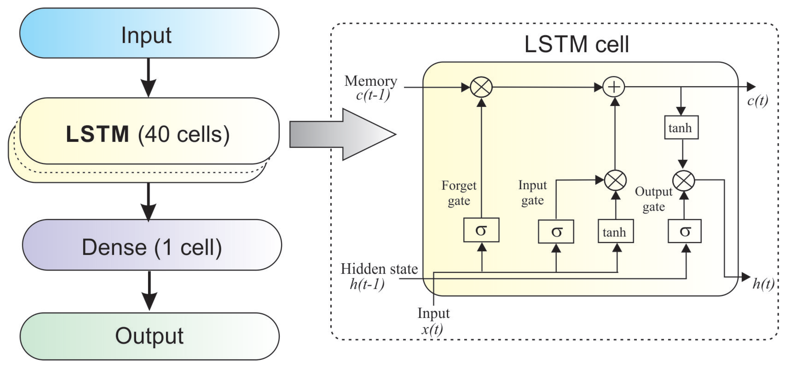
Artificial neural networks (ANNs) with integrated LSTM cells [29] are employed to perform the forecasting task. The LSTM architecture captures temporal dependencies across the input sequences and transmits the learned information to a fully connected layer, where each output node produces a single forecasted value. The dimensions of the input of the ANNs are the number of input time steps and the number of input variables. Figure 1 illustrates the architecture of the forecasting module. Figure 2 presents the overall structure of the artificial neural networks, along with a detailed schematic of the LSTM cells. Each LSTM unit consists of a memory block and three primary gates—input, output, and forget—that regulate information flow. This architecture enables the network to learn long-term dependencies by selectively retaining or discarding temporal information. Specifically, the input gate updates the cell’s content, while the forget gate determines what information in the memory state should be kept or discarded at any given moment. At the same time, the output gate manages the information that is passed from the memory unit. Rectangular boxes represent activation functions applied after matrix multiplication, while circular spots indicate element-wise operations. In Figure 2, x ( t ) , h ( t ) , and c ( t ) correspond to the input, hidden state, and cell activation vector, respectively, with σ denoting the sigmoid activation function. The cell’s output is a weighted sum of x ( t ) , h ( t 1 ) , and a bias term, passed through a sigmoid activation [30].
Multi-step ahead forecasting is accomplished through iterative application of an auto-regressive procedure across the forecasting horizon. In the final stage, the forecasted modes are recombined by summing the outputs of the individual ANNs, yielding the predicted values of the target variable in the multi-channel time series.

2.3. Case Study Framework

This study utilized multi-channel time series data collected from a large passenger ship’s electrical power consumption. The vessel employs an Integrated Power System (IPS) architecture [31], where a centralized diesel–electric plant supplies all onboard power requirements, including both service and propulsion needs [32].
The ship’s electrical distribution network consists of an 11 kV AC primary system powering air conditioning, propulsion, and bow thrusters, complemented by a 690/220 V AC secondary system serving accommodation areas, galleys, and auxiliary services, as illustrated in Figure 3.
Power measurements were recorded at the ship’s high voltage main switchboard connection points (highlighted in Figure 3) over approximately four months with ten-minute sampling intervals. Each dataset channel corresponded to a specific shipboard electrical load.
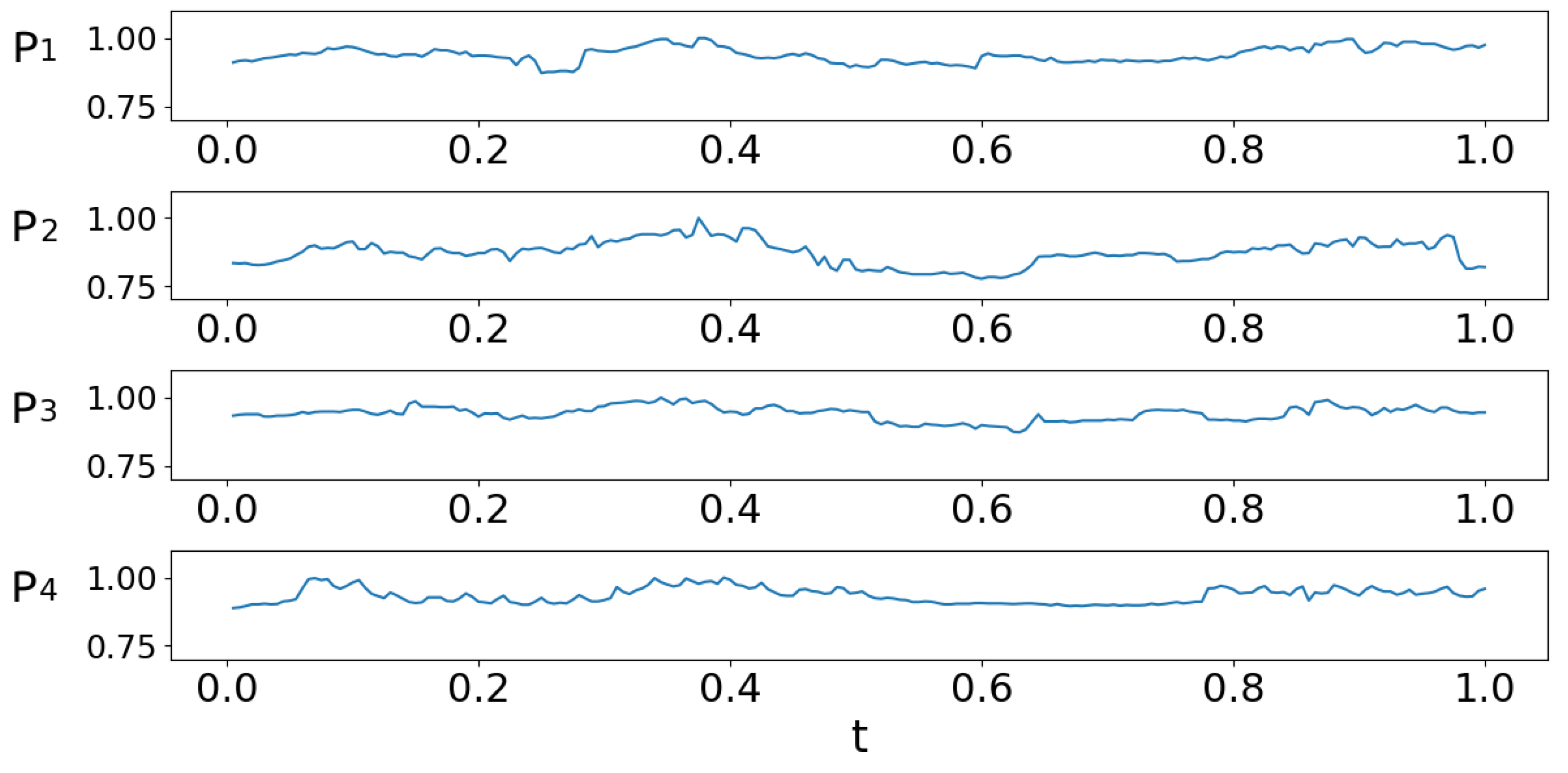
For our analysis, we selected four variables from the electrical load time series—designated as P 1 , P 2 , P 3 , and P 4 —to serve as the channels of the time series. Each variable comprised 17,569 data points (spanning roughly 122 days) that were normalized to the range [ 0.5 ,   0.5 ] before processing. Figure 4 illustrates a 200-time-step window of the four electrical power time series under consideration, normalized.

2.3.1. Causation and Correlation Among the Data Channels

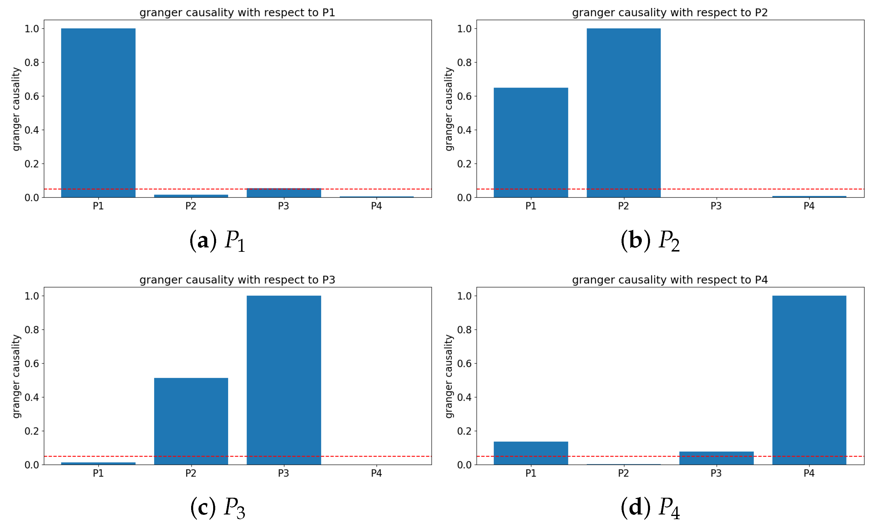
The data channels employed in this study demonstrated weak causality and correlations, which could be quantified using various coefficients. In this analysis, we utilized Granger coefficients to assess causality. Figure 5 presents the results of this assessment. Since Granger causality is designed to measure cross-causality, self-causality was normalized to 1. All values below the conventional Granger threshold (indicated by the dotted horizontal line in the figures) suggested a causal relationship with the respective channel.
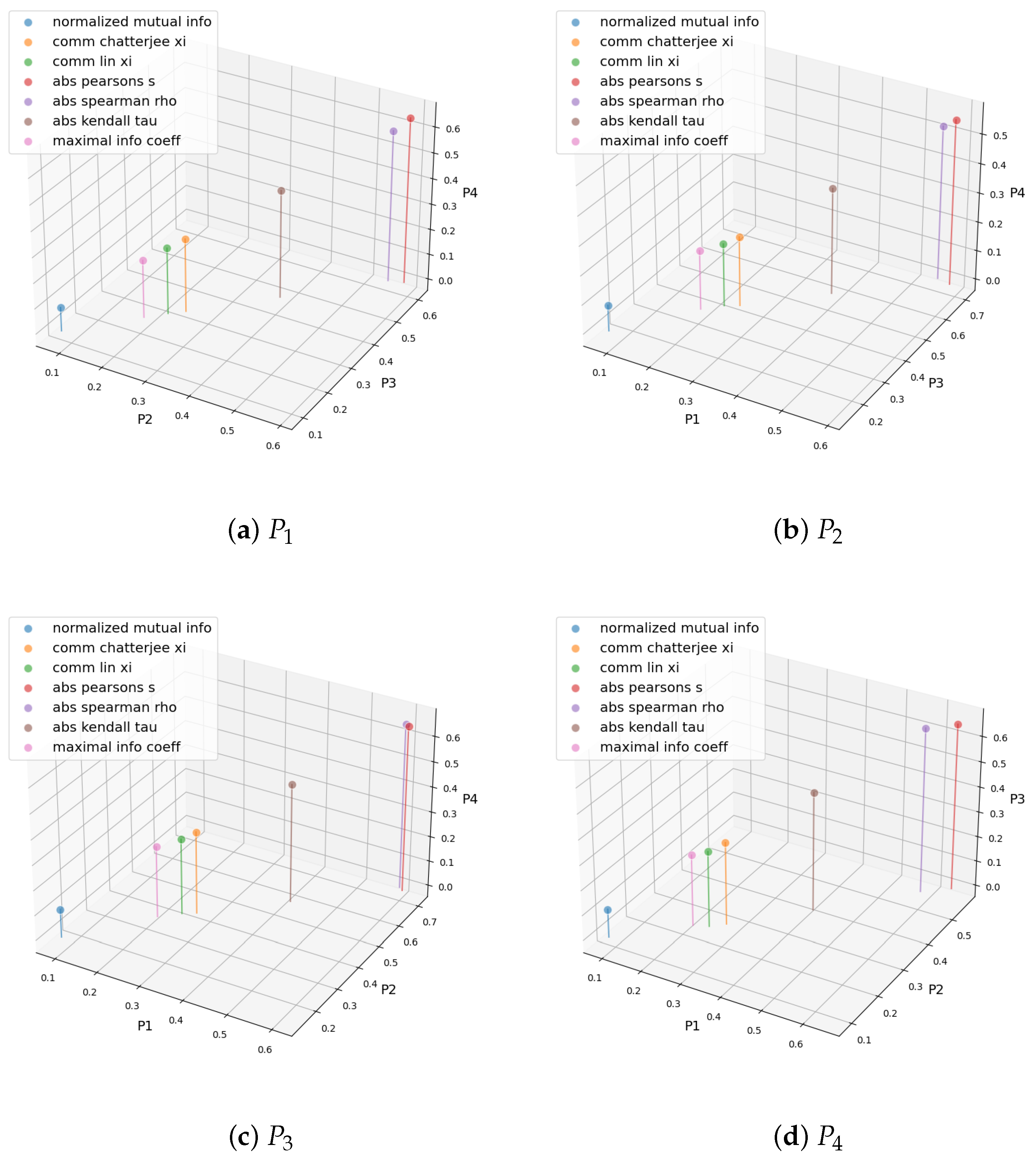
In this study, correlation was assessed using a range of well-established measures, including Pearson, Spearman, Kendall, and normalized mutual information, as well as more recent indices such as Chatterjee’s rank correlation [33], Lin’s coefficient [34], and the maximal information coefficient (MIC) [35]. As illustrated in Figure 6, the choice of correlation metric significantly influenced the interpretation, with several coefficients revealing a non-negligible degree of shared information among the data channels.
The weak but non-negligible causation and correlation observed across the data channels justified adopting a multi-channel scheme for forecasting. These relationships could be exploited through the productive interaction between the resulting modes of the decomposition and the learning process. Specifically, aligning the central frequencies of cooperating modes facilitated the learning task by enabling easier convergence of the optimization problem during training.

2.3.2. Prediction Module Setup

The artificial neural network hyperparameters and VMD parameters followed the values detailed in [7], which were determined using the first 8 h time window of P 1 as a validation set. These values were subsequently confirmed in [28], with the sole modification that Early Stopping was enabled during training. This latest configuration was adopted without modification for the present study, including the method of feeding the four input sequences to the ANN (parallel) and the training specifics, which involved using the Adam optimizer with the default learning rate (0.001) and a batch size of 40.
A similar strategy was employed to determine the number of modes [7].
The β value employed in this study was determined through comprehensive experiments conducted in the foundational work on NCVMD [27]. These experiments evaluated performance across diverse signal types, including the dataset utilized in the present study, and established an optimal balance between decomposition accuracy and central frequency alignment.
Since no additional parameter or hyperparameter tuning was performed for the algorithm presented in this study, all observations were reserved for testing purposes.
The number of modes K was set to 12, representing a balance between reconstruction accuracy and computational complexity. Central frequencies were initialized with six values uniformly spaced in the interval [ 0 ,   0.5 ] and six values randomly positioned within [ 0.25 ,   0.5 ] . Additional parameters included α = 2000 , β = 1200 (for auxiliary channels), τ = 1 , and ϵ = exp ( 7 ) , with the ADMM maximum iteration count set to 500.
Four test scenarios were established, each designating one of the four variables as the forecasting target using our proposed methodology. The artificial neural network structure, depicted in Figure 2, was trained using the first 121 days of data, with each time step corresponding to 10 min. The final day in each scenario was segmented into three consecutive 8 h periods (time slots 1, 2, and 3) for testing purposes. In total, the proposed method was evaluated using twelve test sets of 48 time steps each.
Each scenario was benchmarked against LSTM models with three different preprocessing approaches: single-channel VMD (one-to-one forecasting using past values of a single time series), MVMD, and VMDMS [28].
Table 1 presents the hyperparameters used in the ANN design, based on configurations from previous work [27,28].

3. Results

3.1. Decomposition in the Frequency Domain

As demonstrated in [7], conventional prediction methods applied to the given dataset result in suboptimal performance. Consequently, we adopted decomposition-based approaches. The decomposition of the four electrical power time series variables collected from the case study ship ( P 1 , P 2 , P 3 , and P 4 ) was carried out under the conditions specified in Section 2.3.
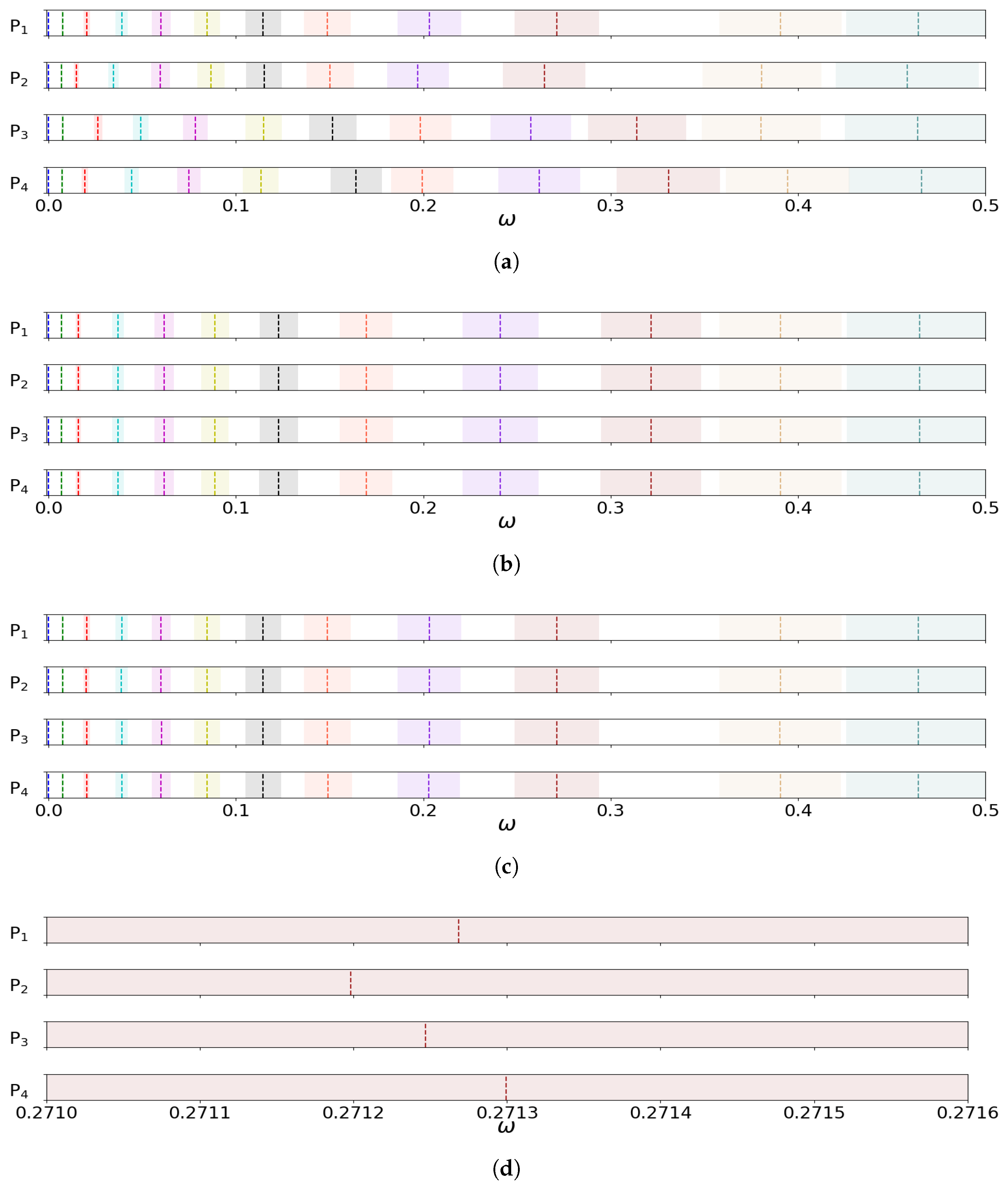
Figure 7 presents a set of graphs illustrating the K = 12 modes generated for each of the four variables under consideration, represented in the frequency domain. Graph (a) depicts VMD (and VMDMS, which produces an identical decomposition), generating non-aligned modes. Graph (b) shows NCVMD, which aligned the modes of the auxiliary channels with those of the main channel, here considered as the first channel: by design, in NCVMD, the P 1 representation was identical to that of VMD and VMDMS, while the representations of the other P i ( i = 2 4 ) channels’ modes approximately aligned with P 1 . Finally, Graph (c) illustrates MVMD, which perfectly aligned the modes’ central frequencies without prioritizing any particular channel, while Graph (d) shows a zoomed-in version of Graph (b) that highlights the misalignment among the central frequencies.

3.2. Forecasting Results

The accuracy of the proposed forecasting method was evaluated under the conditions described in Section 2.3. Benchmarks for assessing the performance of NCD-Pred were constructed using the same machine learning framework, differing only in the pre-processing decomposition module, which was varied among VMD, MVMD, and VMDMS in place of the NCVMD utilized in NCD-Pred. For clarity and brevity, these forecasting systems are referred to by their respective decomposition methods throughout this section, avoiding further definitions.
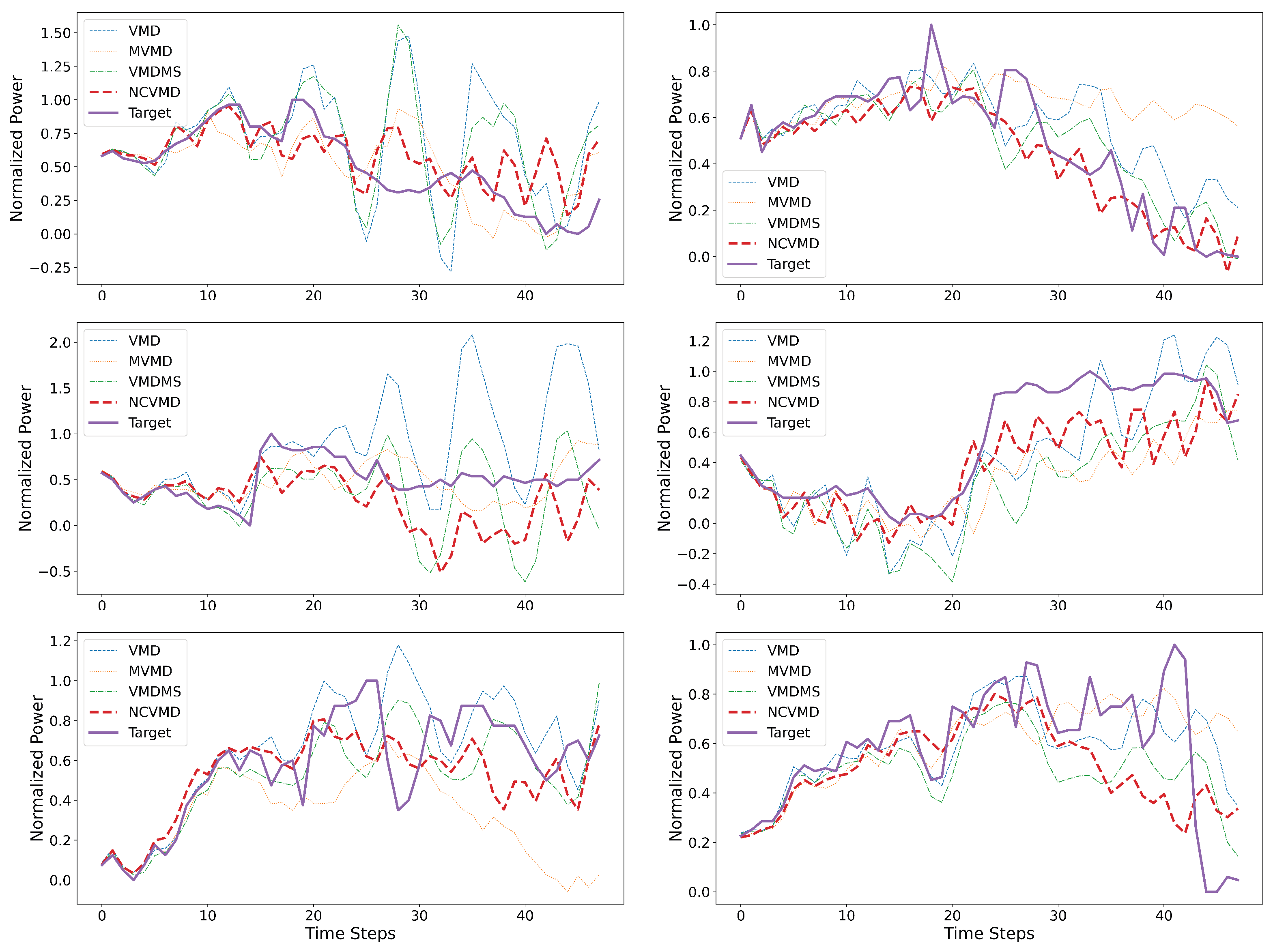
Multi-step ahead forecasting results for the powers P 1 and P 2 are given in Figure 8. The evaluation period spanned 24 h, partitioned into three 8 h time slots (labeled time slots 1, 2, and 3), corresponding to a 48-step forecasting horizon. To ensure operational data confidentiality, the power values shown in Figure 8 were normalized by the respective maximum observed values of P 1 and P 2 over the test duration. In each graph, the violet line represents observation (Target), the blue line depicts the result of VMD, the orange line depicts the results of MVMD, the green line represents VMDMS, and the red line depicts the results of NCD-Pred.
To quantitatively evaluate the accuracy of the proposed method, the Normalized Root Mean Squared Error (NRMSE), Normalized Mean Absolute Error (NMAE), and Symmetric Mean Absolute Percentage Error (sMAPE) were computed across all considered test scenarios. The formulae of these error metrics are provided in Equations (9)–(11). NRMSE emphasizes larger errors due to its squaring of residuals; NMAE provides a more straightforward interpretation by averaging the absolute errors, making it less sensitive to outliers; while sMAPE offers a symmetric perspective on percentage errors, balancing the impact of over- and under-forecasting. These complementary metrics helped to provide a more general understanding of the forecasting performance:
NRMSE = 100 1 n t = 1 n ( f t o t ) 2 o ˜
NMAE = 100 n t = 1 n | f t o t | o ˜
sMAPE = 100 n t = 1 n | f t o t | ( | f t | + | o t | ) 2
where o t is the observation (target), f t is the forecast, and o ˜ = max t [ 1 , n ] ( o t ) .
The obtained results are summarized in Table 2, Table 3 and Table 4, where table cells are color-coded using a heatmap: within each row, the best performances (lowest errors) are highlighted in white, the second-best in light red, and the highest errors in dark red. Analysis of the metrics confirms that the proposed NCD-Pred achieved a clear performance improvement over the benchmark methods. Across all adopted metrics, NCD-Pred produced the lowest forecasting error in six out of twelve instances, compared to two instances for the competing methods.

4. Discussion

This paper describes a forecasting system for accurate shipboard electric load forecasting, useful for ship energy management, a critical area for optimizing efficiency in large passenger ships, and aligned with recent international decarbonization policies.
The main focus of this work was to report the design of NCD-Pred, a novel methodology for multi-step-ahead forecasting, which combines NCVMD—a recently developed technique for multi-channel time series decomposition [27]—with an ANN architecture and an iterative approach for multi-step forecasting. NCD-Pred utilizes NCVMD to (1) establish a hierarchy within the multi-channel input signal, prioritizing the most informative channel (the main channel), which contains the critical forecasting information, while grouping the remaining channels as auxiliary sources of information, and (2) decompose multi-channel time series such that corresponding modes share similar regions in the frequency domain, facilitating the processing of aligned modes for forecasting purposes. Following decomposition, the resulting components are used as inputs for an LSTM-based forecasting model, whose outputs are subsequently recomposed to generate the overall power time series prediction.
To evaluate the proposed approach, we conducted extensive tests using electric load power time series data from a large, real-world passenger ship. Our tests indicate an improvement in overall forecasting performance by NCD-Pred compared to benchmark approaches based on VMD, MVMD [18], and VMDMS [28].
A key aspect of the algorithm is its applicability in real-world scenarios, such as energy management systems aboard ships. Although the decomposition and re-composition costs of NCVMD are comparable to those of VMD and other benchmarks—and are, in fact, negligible—the critical aspect lies in the number of modes into which the original signal is decomposed. Each mode effectively becomes a separate forecasting problem that requires training every 24 h (for a 24 h horizon composed of three consecutive 8 h windows). In the cases examined in [7,28] and in this study, the number of modes, K = 12, struck a good balance between simplifying the forecasting task and avoiding an excessive proliferation of forecasting problems: training requires approximately 8.3 min per time series, which is compatible with the requirement of performing daily retraining (every 24 h). Moreover, this value of K = 12 performed consistently well across all considered decomposition methods (VMD, MVMD, and NCVMD) when the update rate τ = 1 , as specified in [27]. The experiments were conducted using the following hardware configuration: Processor: 12th Gen Intel® Core i7-12850HX (24 cores, max 4.8 GHz); Architecture: x86_64 (64-bit); RAM: 62 GiB; Graphics: NVIDIA GPU (driver: nvidia, resolution: 1920 × 1080); VT-x supported.
Future research will focus on analyzing statistical characteristics such as information content, entropy, sensitivity to weak causation and correlation among channels, and the potential presence of outliers. This line of inquiry will be particularly valuable for cases where NCD-Pred outcomes underperform compared to the benchmark, helping to determine whether further improvements are achievable. Additionally, an advanced approach could involve combining various decomposition methods into an integrated solution, leveraging their respective strengths. This strategy aims to create a unified framework that harnesses the unique capabilities of each method to enhance overall performance.
NCD-Pred utilizes NCVMD to conduct forecasting using multi-channel inputs, avoiding restrictive assumptions about the data’s structure. This approach broadens the potential applications of NCVMD in multi-channel time series prediction. In future experiments, we plan to apply the presented algorithm to multi-channel datasets with diverse physical characteristics and statistical properties, aiming to refine our understanding of its limitations and potential.

Author Contributions

P.F.: Conceptualization, Investigation, Methodology, Software, Visualization, Writing—original draft, Writing—review and editing; G.L.T.: Conceptualization, Data curation, Validation, Writing—original draft, Writing—review and editing; M.M.: Conceptualization, Data curation, Validation, Writing—original draft, Writing—review and editing; M.D.: Funding acquisition, Conceptualization, Supervision, Writing—review and editing; M.C.D.P.: Conceptualization, Data curation, Funding acquisition, Project administration, Supervision, Validation, Writing—original draft, Writing—review and editing. All authors have read and agreed to the published version of the manuscript.

Funding

This research was funded by the Italian Ministry of University and Research (MUR) under the following grant: Sustainable Mobility Center (CNMS) Spoke 3, project id CN00000023, CUP: B43C22000440001.

Data Availability Statement

The data that support the findings of this study are available from the Fincantieri Group, but restrictions apply to the availability of these data, which were used under license for the current study and so are not publicly available. Data are, however, available from the authors upon reasonable request to the corresponding author and with the permission of the Fincantieri Group.

Acknowledgments

The authors would like to thank the Fincantieri Group for providing the shipboard electrical power consumption dataset and for the fruitful collaboration within the scope of the project that funded this research.

Conflicts of Interest

The authors declare no conflicts of interest.

References

  1. Rahimi, N.; Park, S.; Choi, W.; Oh, B.; Kim, S.; Cho, Y.h.; Ahn, S.; Chong, C.; Kim, D.; Jin, C.; et al. A Comprehensive Review on Ensemble Solar Power Forecasting Algorithms. J. Electr. Eng. Technol. 2023, 18, 719–733. [Google Scholar] [CrossRef] [PubMed]
  2. Dragomiretskiy, K.; Zosso, D. Variational Mode Decomposition. IEEE Trans. Signal Process. 2014, 62, 531–544. [Google Scholar] [CrossRef]
  3. Huang, N.E.; Shen, Z.; Long, S.R.; Wu, M.C.; Shih, H.H.; Zheng, Q.; Yen, N.C.; Tung, C.C.; Liu, H.H. The empirical mode decomposition and the Hilbert spectrum for nonlinear and non-stationary time series analysis. Proc. R. Soc. Lond. A 1998, 454, 903–995. [Google Scholar] [CrossRef]
  4. Haykal, V.; Cardot, H.; Ragot, N. A Combination of Variational Mode Decomposition with Neural Networks on Household Electricity Consumption Forecast. In Proceedings of the ITISE 2017, Granada, Spain, 18–20 September 2017. [Google Scholar]
  5. Chao, H.C.; Lin, F.I.; Pan, J.S.; Chien, W.T.; Lai, C.S. Power Load Forecasting Based on VMD and Attention-LSTM. In Proceedings of the 3rd International Conference On Data Science And Information Technology, Xiamen, China, 24–26 July 2020; pp. 19–25. [Google Scholar] [CrossRef]
  6. Huang, Y.; Huang, Z.; Yu, J.; Dai, X.; Li, Y. Short-term load forecasting based on IPSO-DBiLSTM network with variational mode decomposition and attention mechanism. Appl. Intell. 2023, 53, 12701–12718. [Google Scholar] [CrossRef]
  7. Fazzini, P.; La Tona, G.; Diez, M.; Di Piazza, M.C. Sailing Towards Efficiency: A Variational Mode Decomposition Based Approach to Forecasting Shipboard Electrical Power Consumption. In Proceedings of the 2024 IEEE International Conference on Electrical Systems for Aircraft, Railway, Ship Propulsion and Road Vehicles & International Transportation Electrification Conference (ESARS-ITEC), Naples, Italy, 26–29 November 2024; pp. 1–6. [Google Scholar] [CrossRef]
  8. Zhou, F.; Zhou, H.; Li, Z.; Zhao, K. Multi-Step Ahead Short-Term Electricity Load Forecasting Using VMD-TCN and Error Correction Strategy. Energies 2022, 15, 5375. [Google Scholar] [CrossRef]
  9. Zhang, Q.; Wu, J.; Ma, Y.; Li, G.; Ma, J.; Wang, C. Short-term load forecasting method with variational mode decomposition and stacking model fusion. Sustain. Energy Grids Netw. 2022, 30, 100622. [Google Scholar] [CrossRef]
  10. Xiong, Q.; Liu, M.; Li, Y.; Zheng, C.; Deng, S. Short-Term Load Forecasting Based on VMD and Deep TCN-Based Hybrid Model with Self-Attention Mechanism. Appl. Sci. 2023, 13, 12479. [Google Scholar] [CrossRef]
  11. Zhang, Z.; Hong, W.; Li, J. Electric Load Forecasting by Hybrid Self-Recurrent Support Vector Regression Model With Variational Mode Decomposition and Improved Cuckoo Search Algorithm. IEEE Access 2020, 8, 14642–14658. [Google Scholar] [CrossRef]
  12. Zhang, D.; Peng, X.; Pan, K. A Novel Online Method for Wind Speed Forecasting Based on Hybrid Decomposition and OSORELM. In Proceedings of the 2018 International Conference On Power System Technology (POWERCON), Guangzhou, China, 6–9 November 2018; pp. 1797–1804. [Google Scholar] [CrossRef]
  13. Xia, X.; Wang, X. A Novel Hybrid Model for Short-Term Wind Speed Forecasting Based on Twice Decomposition, PSR, and IMVO-ELM. Complexity 2022, 2022, 1–21. [Google Scholar] [CrossRef]
  14. Alemu, N.S.; Zheng, D.; Zhang, W.; Teshager, G. Short-term PV power forecasting using variational mode decomposition integrated with Ant colony optimization and neural network. Energy Rep. 2022, 8, 2022–2035. [Google Scholar] [CrossRef]
  15. Wang, Z.; Liu, Y.; Du, J.; Wang, Z.; Shao, Q. De-noising magnetotelluric data using variational mode decomposition combined with mathematical morphology filtering and wavelet thresholding. J. Appl. Geophys. 2022, 204, 104751. [Google Scholar] [CrossRef]
  16. Shi, J.; Zhou, J.; Feng, J.; Chen, H. Network traffic prediction model based on improved VMD and PSO-ELM. Int. J. Commun. Syst. 2023, 36, e5448. [Google Scholar] [CrossRef]
  17. Wang, Z.; Gao, R.; Wang, P.; Chen, H. A new perspective on air quality index time series forecasting: A ternary interval decomposition ensemble learning paradigm. Technol. Forecast. Soc. Change 2023, 191, 122504. [Google Scholar] [CrossRef]
  18. Rehman, N.; Aftab, H. Multivariate Variational Mode Decomposition. IEEE Trans. Signal Process. 2019, 67, 6039–6052. [Google Scholar] [CrossRef]
  19. Huang, Y.; Hasan, N.; Deng, C.; Bao, Y. Multivariate empirical mode decomposition based hybrid model for day-ahead peak load forecasting. Energy 2022, 239, 122245. [Google Scholar] [CrossRef]
  20. Rehman, N.; Mandic, D.P. Multivariate Empirical Mode Decomposition. Proc. R. Soc. A 2010, 466, 1291–1302. [Google Scholar] [CrossRef]
  21. International Maritime Organization (IMO). Fourth IMO GHG Study 2020 Full Report; International Maritime Organization (IMO): London, UK, 2021; Volume 6, pp. 951–952. [Google Scholar]
  22. DNV-GL. MARITIME FORECAST TO 2050—Energy Transition Outlook 2019; Technical Report; DNV-GL: Oslo, Norway, 2019. [Google Scholar]
  23. IMO. IMO Action to Reduce Greenhouse Gas Emissions from International Shipping; International Maritime Organization (IMO): London, UK, 2019. [Google Scholar]
  24. Lee, H.; Lee, J.; Roh, G.; Lee, S.; Choung, C.; Kang, H. Comparative Life Cycle Assessments and Economic Analyses of Alternative Marine Fuels: Insights for Practical Strategies. Sustainability 2024, 16, 2114. [Google Scholar] [CrossRef]
  25. Nivolianiti, E.; Karnavas, Y.L.; Charpentier, J.F. Energy management of shipboard microgrids integrating energy storage systems: A review. Renew. Sustain. Energy Rev. 2024, 189, 114012. [Google Scholar] [CrossRef]
  26. Di Piazza, M.; La Tona, G.; Luna, M.; Di Piazza, A. A two-stage Energy Management System for smart buildings reducing the impact of demand uncertainty. Energy Build. 2017, 139, 1–9. [Google Scholar] [CrossRef]
  27. Fazzini, P.; La Tona, G.; Diez, M.; Montuori, M.; Di Piazza, M.C. Multi-Channel Neighborhood-Constrained Variational Mode Decomposition. TechRxiv 2025. [Google Scholar] [CrossRef]
  28. Fazzini, P.; La Tona, G.; Diez, M.; Di Piazza, M.C. Enhanced forecasting of shipboard electrical power demand using multivariate input and variational mode decomposition with mode selection. Sci. Rep. 2025, 15, 23941. [Google Scholar] [CrossRef]
  29. Hochreiter, S. Long Short-term Memory. Neural Comput. 1997, 8, 1735–1780. [Google Scholar] [CrossRef]
  30. Fazzini, P.; Montuori, M.; Pasini, A.; Cuzzucoli, A.; Crotti, I.; Campana, E.F.; Petracchini, F.; Dobricic, S. Forecasting PM10 Levels Using Machine Learning Models in the Arctic: A Comparative Study. Remote Sens. 2023, 15, 3348. [Google Scholar] [CrossRef]
  31. Sulligoi, G.; Vicenzutti, A.; Menis, R. All-Electric Ship Design: From Electrical Propulsion to Integrated Electrical and Electronic Power Systems. IEEE Trans. Transp. Electrif. 2016, 2, 507–521. [Google Scholar] [CrossRef]
  32. Patel, M.R. Shipboard Electrical Power Systems; CRC Press: Boca Raton, FL, USA, 2021. [Google Scholar]
  33. Chatterjee, S. A New Coefficient of Correlation. J. Am. Stat. Assoc. 2021, 116, 2009–2022. [Google Scholar] [CrossRef]
  34. Lin, Z.; Han, F. On boosting the power of Chatterjee’s rank correlation. Biometrika 2022, 110, 283–299. [Google Scholar] [CrossRef]
  35. Reshef, D.N.; Reshef, Y.A.; Finucane, H.K.; Grossman, S.R.; McVean, G.; Turnbaugh, P.J.; Lander, E.S.; Mitzenmacher, M.; Sabeti, P.C. Detecting Novel Associations in Large Data Sets. Science 2011, 334, 1518–1524. [Google Scholar] [CrossRef]
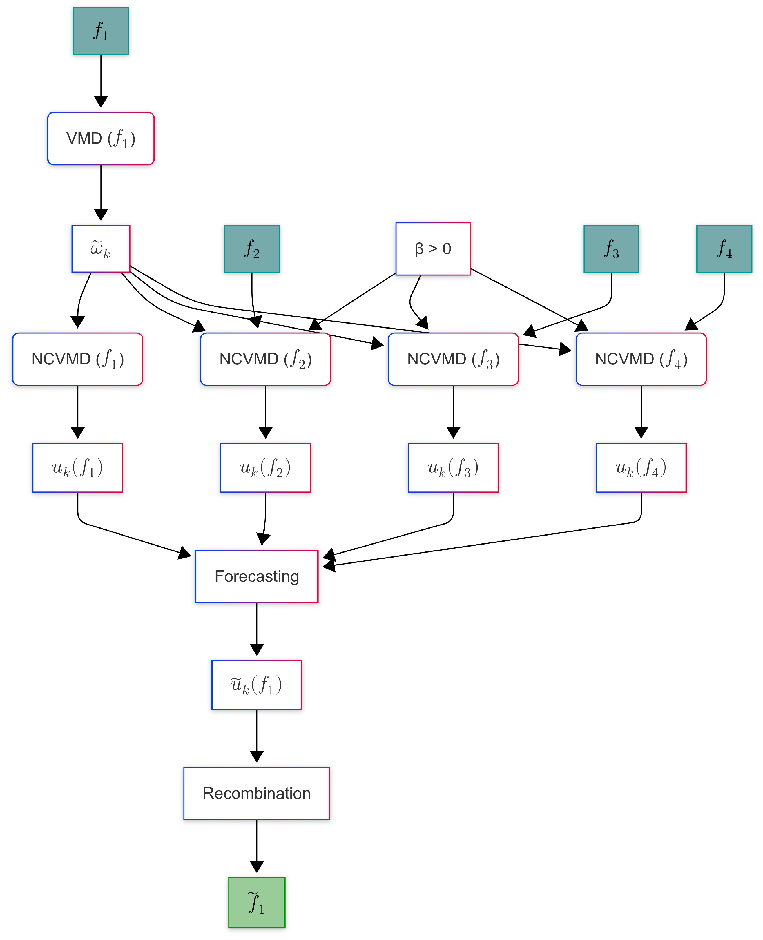
Figure 1. NCD-Pred: overall structure of the forecasting apparatus.
Forecasting 07 00044 g001
Figure 2. Overall structure of the ANNs and the detailed structure of LSTM cells as detailed in [27].
Forecasting 07 00044 g002
Figure 3. Electrical power system [7].
Forecasting 07 00044 g003
Figure 4. Shipboard electrical power demand dataset ( P 1 4 ), normalized.
Forecasting 07 00044 g004
Figure 5. Pairwise Granger coefficients among P 1 , P 2 , P 3 , and P 4 . The dotted horizontal line indicates the Granger threshold.
Forecasting 07 00044 g005
Figure 6. This figure of four 3D scatter plots represents the pairwise correlation coefficients among P 1 , P 2 , P 3 , and P 4 . Each plot is dedicated to one of these parameters. In each plot, the coordinates of a point indicate the correlation of the dedicated parameter with the other three. Specifically, in the P 1 plot, the X, Y, and Z coordinates of a point represent the correlation of P 1 with P 2 , P 3 , and P 4 , respectively. In the P 2 plot, the coordinates represent the correlation of P 2 with P 1 , P 3 , and P 4 , and so on for the P 3 and P 4 plots.
Forecasting 07 00044 g006
Figure 7. Frequency representation of modes when P 1 was the NCVMD main channel with a time window of 17,424 time steps, i.e., equal to the length of the train set: (a) VMD and VMDMS, which produced an identical decomposition; (b) MVMD; (c) NCVMD. By design, in NCVMD, the P 1 representation was identical to that of VMD and VMDMS, while the representations of the other P i tended to align approximately with P 1 . Note that across the entire spectrum, the imprecise alignment was not noticeable. However, considering the tenth central frequency and zooming into the frequency interval [0.271, 0.2716], the misalignment became visible, as shown in (d). In contrast with the NCVMD behavior, MVMD achieved perfect alignment without safeguarding any specific channel. The percentage decomposition errors in terms of NRMSE range from 0.3 % to 0.6 % , well within acceptable thresholds for the objectives of this study.
Forecasting 07 00044 g007
Figure 8. Forecasting results for the normalized powers P 1 and P 2 obtained when switching the decomposition module. First column: forecasts for the time slots 1, 2, and 3 of P 1 (top to bottom). Second column: forecasts for the time slots 1, 2, and 3 of P 2 (top to bottom). In the graphs, the violet line represents observation (Target), the blue line depicts the result when the decomposition module was VMD, the orange line depicts the results for MVMD, the green line represents the results for VMDMS, and the red dashed line depicts the results when using NCVMD as the decomposition module (i.e., NCD-Pred). The graphs were normalized by dividing by the maximum observed values of P 1 , P 2 over the 24 h test period.
Forecasting 07 00044 g008
Table 1. Model hyperparameters.
HyperparameterValue
Input steps for each mode150 140 130 120 100 80
60 40 30 25 20 20
Num. of LSTM cells40
Epochs5
Early Stoppingyes
Dense layer activationtanh()
Loss0.5 × [Mean Squared Error] +
0.5 × [Mean Cross Entropy]
Table 2. NRMSE forecasting error metrics. Darker shades correspond to larger errors.
Power/SlotVMDMVMDVMDMSNCD-Pred
P 1 —Slot 14.65892.61224.22942.5818
P 1 —Slot 23.62031.39342.42952.2225
P 1 —Slot 31.73842.83721.59221.4231
P 2 —Slot 13.64615.70572.92082.4994
P 2 —Slot 23.00143.79654.07152.6854
P 2 —Slot 32.65912.96442.78493.0040
P 3 —Slot 11.92802.17774.67582.3759
P 3 —Slot 22.40783.18662.10034.1193
P 3 —Slot 32.87071.60333.17762.0501
P 4 —Slot 13.02112.45492.16232.3475
P 4 —Slot 24.78631.31011.97310.7752
P 4 —Slot 36.06002.70434.86441.9290
Table 3. NMAE forecasting error metrics. Darker shades correspond to larger errors.
Power/SlotVMDMVMDVMDMSNCD-Pred
P 1 —Slot 13.26261.95282.91841.8662
P 1 —Slot 22.36331.13931.77581.7492
P 1 —Slot 31.09692.19901.12001.0671
P 2 —Slot 12.85443.93732.16561.8151
P 2 —Slot 22.37702.92993.35182.1180
P 2 —Slot 31.74551.88572.07992.0606
P 3 —Slot 11.48451.65523.69631.7773
P 3 —Slot 21.83592.05301.57782.7812
P 3 —Slot 32.18581.14482.38561.6204
P 4 —Slot 12.25291.61421.47181.6652
P 4 —Slot 23.30680.97361.55540.5938
P 4 —Slot 34.53941.79583.37221.3942
Table 4. SMAPE forecasting error metrics. Darker shades correspond to larger errors.
Power/SlotVMDMVMDVMDMSNCD-Pred
P 1 —Slot 13.41162.06263.05531.9761
P 1 —Slot 22.36911.17211.84611.8225
P 1 —Slot 31.12052.28931.15091.0996
P 2 —Slot 13.18954.41602.40752.0190
P 2 —Slot 22.51113.07603.57912.2223
P 2 —Slot 31.85462.00612.20582.1954
P 3 —Slot 11.54171.71763.77451.8458
P 3 —Slot 21.94582.16121.63732.9368
P 3 —Slot 32.24461.19002.43451.7018
P 4 —Slot 12.33081.67461.52281.7322
P 4 —Slot 23.28931.00641.60720.6115
P 4 —Slot 34.57521.81363.43721.4185
Disclaimer/Publisher’s Note: The statements, opinions and data contained in all publications are solely those of the individual author(s) and contributor(s) and not of MDPI and/or the editor(s). MDPI and/or the editor(s) disclaim responsibility for any injury to people or property resulting from any ideas, methods, instructions or products referred to in the content.