Abstract
Hyperparameter optimization (HPO) is critical for enhancing the predictive performance of machine learning models in credit risk assessment for peer-to-peer (P2P) lending. This study evaluates four HPO methods, Grid Search, Random Search, Hyperopt, and Optuna, across four models, Logistic Regression, Random Forest, XGBoost, and LightGBM, using three real-world datasets (Lending Club, Australia, Taiwan). We assess predictive accuracy (AUC, Sensitivity, Specificity, G-Mean), computational efficiency, robustness, and interpretability. LightGBM achieves the highest AUC (e.g., on Lending Club, on Australia, on Taiwan), with XGBoost performing comparably. Bayesian methods (Hyperopt, Optuna) match or approach Grid Search’s accuracy while reducing runtime by up to -fold (e.g., vs. min for LightGBM on Lending Club). A sensitivity analysis confirms robust hyperparameter configurations, with AUC variations typically below under perturbations. A feature importance analysis, using gain and SHAP metrics, identifies debt-to-income ratio and employment title as key default predictors, with stable rankings (Spearman correlation ) across tuning methods, enhancing model interpretability. Operational impact depends on data quality, scalable infrastructure, fairness audits for features like employment title, and stakeholder collaboration to ensure compliance with regulations like the EU AI Act and U.S. Equal Credit Opportunity Act. These findings advocate Bayesian HPO and ensemble models in P2P lending, offering scalable, transparent, and fair solutions for default prediction, with future research suggested to explore advanced resampling, cost-sensitive metrics, and feature interactions.
MSC:
91G40; 68T01; 62H25
1. Introduction
Peer-to-peer (P2P) lending, also known as social lending, is an innovative financial service that connects borrowers directly with lenders through online platforms, bypassing traditional intermediaries like banks [1]. By leveraging digital infrastructure and social media, P2P lending enhances access to credit, fostering financial inclusion, particularly for underserved populations.
The availability and regulatory frameworks of P2P lending vary significantly across countries. In the United Kingdom, the P2P lending market is well established and regulated by the Financial Conduct Authority (FCA), with platforms such as Zopa and Funding Circle achieving broad adoption [2]. In the United States, the market is sizable, dominated by Lending Club and Prosper, but operates under a fragmented regulatory landscape governed by both state and federal laws. Several European countries, including Germany, France, and the Netherlands, have embraced P2P lending within specific regulatory regimes, although the market remains modest in scale compared to Anglo-American counterparts. In the Asia-Pacific region, rapid growth is anticipated, with China leading the market. Countries like Japan and South Korea also show steady expansion, supported by robust regulation and a strong culture of financial innovation. In contrast, countries such as Canada and India maintain strict regulatory environments; for instance, Indian platforms must register as non-banking financial companies (NBFCs). In some jurisdictions, such as Pakistan, Indonesia, and parts of the Middle East, P2P lending remains either prohibited or heavily restricted due to regulatory or religious constraints [3].
Globally, the P2P lending market has expanded considerably. Analysts estimate that the total market value may have reached up to USD 490 billion by 2022 and is projected to grow to USD billion by 2030, reflecting a compound annual growth rate (CAGR) of approximately from 2022 to 2030 [4]. North America holds the largest share of the global market, with established platforms like Lending Club and Prosper facilitating loans totaling USD 61 billion between 2018 and 2020. The market is expected to grow to USD 150 billion by 2025 [5]. Europe is also experiencing robust growth, though its overall market size remains smaller than North America’s. The United Kingdom currently ranks as the third-largest P2P lending market globally, following the United States and China [3,6]. In 2017, the UK’s market volume reached EUR billion, with an annual growth rate of since 2011 [5]. Asia-Pacific is the fastest-growing region. China, which once hosted 1553 active platforms and recorded a transaction volume of RMB trillion in 2017 [7], remains the largest market despite recent regulatory crackdowns aimed to limit P2P lending platforms [3]. Other rapidly expanding markets include India, South Korea, and Japan, which is projected to maintain a CAGR of around between 2024 and 2034. These figures highlight the increasing global significance of P2P lending, despite its uneven development across regions.
Nevertheless, P2P lending faces significant challenges, notably information asymmetry and rising default rates, which undermine platform stability and profitability [8,9]. To address these risks, P2P platforms employ internal credit scoring systems, framing credit risk assessment as a binary classification task, with loan repayment status as the target variable (fully repaid loans labeled “1” and defaulted loans “0”) [10]. Traditional creditworthiness evaluation methods, such as Fair Isaac Corporation (FICO) scores and subjective assessments, often fail to capture complex borrower behaviors and non-linear relationships among predictive features. In response, advanced statistical and machine learning models have emerged, offering superior predictive accuracy and interpretability by leveraging high-dimensional borrower data, dynamic credit behaviors, and intricate feature interactions [11,12].
Ensemble learning models, which aggregate predictions from multiple base learners, consistently outperform individual classifiers and traditional statistical approaches in credit risk modeling [12]. However, their effectiveness hinges on hyperparameter optimization, as parameters such as learning rates, tree depths, and regularization terms govern model complexity and generalization. For example, an excessively high learning rate may lead to premature convergence, missing critical default patterns, while overly complex architectures, such as deep decision trees, risk overfitting, reducing generalizability to new loan applications [13].
Exhaustive hyperparameter tuning, such as Grid Search, is computationally intensive, and suboptimal configurations can significantly impair performance. Moreover, hyperparameter tuning strategies influence feature importance stability, which is critical for model interpretability and risk factor prioritization, yet this aspect remains underexplored [14]. The unique characteristics of P2P lending, including simplified underwriting and limited regulatory oversight, exacerbate default risks compared to traditional credit systems [15]. Even marginal improvements in default prediction can significantly enhance platform stability and reduce financial exposure [16,17].
This study addresses these challenges by systematically benchmarking two Bayesian optimization frameworks, Hyperopt [18] and Optuna [19], against conventional methods, Grid Search (GS) and Random Search (RS) [20], to optimize credit risk prediction models. Bayesian optimization offers a computationally efficient alternative to traditional methods, particularly for complex models [21,22]. We evaluate Logistic Regression [23] and ensemble models, including Random Forest [24], XGBoost [25], and LightGBM [26], using the Lending Club (LC) dataset [27], supplemented by the Australia [28] and Taiwan [29] credit card datasets for broader applicability.
Our findings demonstrate that Bayesian optimization methods (Hyperopt and Optuna) achieve predictive performance comparable to Grid Search while reducing computational costs by up to -fold, with Hyperopt being particularly efficient. Models trained with optimized hyperparameters significantly outperform those with default settings, highlighting the critical role of hyperparameter optimization (HPO). Additionally, we provide a comprehensive analysis of hyperparameter tuning’s impact on model performance, sensitivity, and feature importance stability, offering actionable insights for P2P lending platforms to enhance credit scoring efficiency and interpretability.
This research is guided by the following questions:
- Which hyperparameter tuning method offers the optimal balance between computational efficiency and predictive performance for credit scoring in P2P lending?
- How sensitive is model performance to perturbations in optimal hyperparameter configurations?
- How do hyperparameter tuning strategies affect the stability and consistency of model interpretability?
The paper is organized as follows: Section 2 reviews the relevant literature on P2P lending, default prediction, and machine learning applications in credit risk. Section 3 details the methodological approach. Section 4 describes the experimental setup, and Section 5 presents the results. Section 6 concludes with implications for future research.
2. Related Work
Peer-to-peer lending has garnered significant attention for its potential to democratize access to credit by providing faster and more flexible funding solutions. However, the absence of collateral and limited regulatory oversight expose the industry to considerable credit risk, requiring robust methods to accurately predict loan defaults. Traditionally, online financial platforms have relied on quantitative credit scoring systems, such as FICO scores, or proprietary metrics like the Lending Club score. Although these methods offer initial assessments of borrower creditworthiness, they fall short in accurately predicting default risk. Their reliance on general risk scores limits their ability to capture nuanced interactions between variables, leaving investors with insufficient confidence in the borrower’s reliability [30].
In response to these limitations, P2P platforms have begun framing credit evaluation as a binary classification task, where the goal is to predict the likelihood of default based on borrower demographics and financial data. Early studies utilized statistical techniques such as Logistic Regression (LR) and Linear Discriminant Analysis (LDA) [31,32]. While these methods proved effective in identifying key predictive variables, their assumption of linear relationships limited their applicability to complex, high-dimensional datasets.
2.1. Machine Learning for Credit Scoring
Machine learning techniques have emerged as a promising alternative for credit risk prediction [12]. Methods such as decision trees (DTs), support vector machines (SVMs), and artificial neural networks (ANNs) have shown significant improvements in predictive performance [33,34,35]. For example, Teply and Polena [36] conducted a comparative evaluation of several classifiers, including Logistic Regression (LR), Artificial Neural Networks, Support Vector Machines, Random Forests (RF), and Bayesian Networks (BNs), on the Lending Club dataset, spanning 2009–2013. They found that Logistic Regression achieved the highest classification accuracy. However, in a similar analysis of the same dataset, Malekipirbazari and Aksakalli [30] revealed that Random Forests outperformed both Logistic Regression and FICO scores.
Numerous studies have conducted comparative evaluations to identify the best algorithm for these classification tasks. Lessmann et al. [12] assessed several classification techniques across a few credit scoring datasets. Their study explored advanced approaches, such as heterogeneous ensembles, rotation forests, and extreme learning machines, while using robust performance measures like the H-measure and partial Gini index. The findings highlighted the superiority of ensemble models over traditional methods, offering valuable insights for improving credit risk modeling.
Building on these advancements, ensemble learning has become a widely adopted approach. Techniques such as Random Forests and gradient boosting combine multiple base models to enhance predictive accuracy and robustness. By integrating diverse algorithms that evaluate various hypotheses, these models produce more reliable predictions, leading to improved precision [16,17]. Ensemble models are generally categorized into parallel and sequential structures. Parallel ensembles, like Bagging and Random Forests, combine independently trained models to make collective decisions simultaneously. In contrast, sequential ensembles, such as boosting algorithms, iteratively refine models by correcting errors from previous iterations.
Ma et al. [37] highlighted LightGBM’s computational efficiency, showing it achieved comparable accuracy to extreme gradient boosting (XGBoost) while running ten times faster. Similarly, Ko et al. [38] benchmarked three statistical models: Logistic Regression, Bayesian Classifier, and Linear Discriminant Analysis, alongside five machine learning models, decision tree, Random Forest, LightGBM, Artificial Neural Network, and Convolutional Neural Network (CNN), using the Lending Club dataset. Their findings showed that LightGBM outperformed the other models, achieving a improvement in accuracy. However, the study did not consider hyperparameter tuning strategies, which could significantly affect model performance. Additionally, their focus on classification accuracy overlooked computational efficiency, a crucial factor for real-world deployment.
2.2. Challenges in Social Lending Datasets
A persistent challenge in credit scoring is class imbalance, where the majority of loans do not default [10,11]. This imbalance causes models to be biased towards the majority class, leading to reduced sensitivity toward the minority class [38,39]. This issue is particularly critical for predicting defaults, as failing to identify defaulted loans can expose lenders to significant financial risks [11]. Traditional machine learning models often assume equal class distributions and focus on optimizing overall accuracy, rather than prioritizing balanced performance metrics such as Sensitivity, Specificity, or Geometric Mean (G-Mean) [32,40].
Resampling techniques have emerged as effective solutions to address class imbalance [41]. Oversampling methods, like the synthetic minority oversampling technique (SMOTE), generate synthetic examples to augment the minority class, while undersampling reduces the majority class. Krishna Veni and Sobha Rani [40] identified three main reasons why traditional classification algorithms struggle with imbalanced data: (1) they are primarily accuracy-driven, often favoring the majority class; (2) they assume an equal distribution of classes, which is rarely the case in imbalanced datasets; and (3) they treat the misclassification error costs of all classes as equal. To overcome these challenges, the study recommended the use of sampling strategies and cost-sensitive learning techniques. Additionally, alternative performance metrics, such as the confusion matrix, precision, and F1-score, were used to better evaluate models on unbalanced datasets.
In another study, Alam et al. [16] investigated the prediction of credit card default using imbalanced datasets, with a focus on enhancing classifier performance while preserving the interpretability of the model. Using datasets like the South German Credit and Belgium Credit data, the study addressed the challenge of class imbalance through various resampling techniques. Gradient-boosted decision trees (GBDTs) were used as the primary model, with hyperparameter tuning of learning rates and the number of trees to improve predictive accuracy. The K-means SMOTE oversampling technique demonstrated significant improvements in G-Mean, precision, and recall, effectively addressing the issue of class imbalance.
Several studies have specifically utilized the Lending Club dataset for credit risk prediction [22]. Moscato et al. [10] highlighted the bias of machine learning models toward the majority class in imbalanced settings. To counter this, they employed oversampling techniques like SMOTE, alongside undersampling methods. The study demonstrated significant improvements in default prediction by using a Random Forest classifier combined with resampling techniques. Additionally, several explainability methods, such as LIME and SHAP, were incorporated to enhance model transparency.
Similarly, Namvar et al. [32] investigated the effectiveness of resampling strategies combined with machine learning classifiers like Logistic Regression and Random Forest. Their findings underscored the importance of metrics such as G-Mean, which balance Sensitivity and Specificity, in effectively addressing imbalanced datasets. The results indicated that combining Random Forests with random undersampling could be a promising approach for assessing credit risk in social lending markets. Song et al. [15] adopted a different approach by introducing an ensemble-based methodology which leverages multi-view learning and adaptive clustering to increase base learner diversity. This method showed superior Sensitivity and adaptability in default identification, outperforming traditional classifiers in highly imbalanced settings.
While addressing class imbalance is crucial, it is not sufficient for optimizing predictive performance in P2P lending datasets due to the complexities introduced by the high dimensionality and intricate feature interactions. Hyperparameter tuning offers a complementary approach that improves model Sensitivity and accuracy. Huang and Boutros [42] highlighted that optimal hyperparameters often vary across datasets, underscoring the importance of tailoring tuning strategies to the specific characteristics of each dataset.
Among existing approaches, Bayesian hyperparameter optimization has proven a more effective alternative, consistently outperforming traditional Grid Search in various empirical studies [43,44]. Chang et al. [45] emphasized the effectiveness of combining models, such as Random Forests and Logistic Regression, to predict loan defaults. Their analysis, using the Lending Club dataset from 2007 to 2015, found that Logistic Regression, enhanced with misclassification penalties and Gaussian Naive Bayes, achieved competitive performance, with Naive Bayes showing the highest Specificity. The study also highlighted the crucial role of hyperparameter tuning, especially for SVMs, where kernel selection and regularization parameters significantly impact model performance.
Xia et al. [22] aimed to develop an accurate and interpretable credit scoring model using XGBoost, with a focus on hyperparameter tuning and sequential model building. Using datasets from a publicly available credit scoring competition that featured class imbalance, the authors employed Bayesian optimization, specifically the tree-structured Parzen estimator (TPE), for adaptive hyperparameter tuning. This method significantly improved SVM performance compared to manual tuning, Grid Search, and Random Search. Bayesian optimization yielded approximately higher performance than grid and manual searches, and 3% higher than Random Search. Additionally, the study examined feature importance based on TPE-optimized models. However, the research did not explore whether different hyperparameter optimization methods affected feature rankings.
3. Methodology
Ensemble learning models, such as Random Forest, XGBoost, and LightGBM, are robust classifiers whose predictive performance depends critically on hyperparameter configuration. This study employed four hyperparameter optimization methods, Grid Search, Random Search, Hyperopt, and Optuna, to tune multiple classification models, including Logistic Regression, Random Forest, XGBoost, and LightGBM. GS and RS served as baselines, with identical search spaces defined for all methods to ensure fair comparison. The experimental workflow, illustrated in Figure 1, encompassed data preprocessing, feature selection, hyperparameter tuning, model training, and evaluation.

Figure 1.
Workflow of the experimental design for credit risk prediction with hyperparameter tuning.
Data preprocessing addressed key challenges in P2P lending datasets, including missing values, redundancy, and class imbalance. Features with excessive missing values were removed, and redundant attributes were eliminated based on correlation analysis and domain knowledge, retaining only the most informative features. Numerical variables were standardized using a robust scaler to mitigate outlier effects, and multicollinearity was assessed via a variance inflation factor analysis to ensure feature independence. Ordinal variables were encoded using integer encoding to preserve their order, while categorical variables were encoded using one-hot encoding, with missing or invalid entries for both treated as distinct categories. To optimize computational efficiency, feature data types were refined (e.g., converting misclassified floats to integers), reducing memory usage. Class imbalance, prevalent in credit risk datasets, was addressed through random undersampling of the training set to achieve a balanced class distribution. The test set retained its original distribution to reflect real-world lending scenarios, ensuring realistic evaluation metrics. Feature selection was then applied using techniques such as recursive feature elimination to filter out low-importance features, reducing dimensionality while preserving predictive power.
Hyperparameter tuning optimized model performance using four methods: GS exhaustively evaluated all combinations within predefined grids; RS randomly sampled configurations from the same search space; Hyperopt and Optuna leveraged Bayesian optimization with tree-structured Parzen estimators (TPEs) to iteratively focus on promising regions, incorporating pruning to terminate unpromising trials early. Search spaces were model-specific (e.g., learning_rate, max_depth for XGBoost; n_estimators, min_samples_split for Random Forest), as detailed in the experimental setup (Section 4).
Post-tuning, models were trained on the preprocessed training set using optimized hyperparameters and the selected feature subset. Performance was evaluated on the test set using metrics tailored for imbalanced datasets: Area Under the Receiver Operating Characteristic Curve (AUC), Sensitivity, Specificity, and Geometric Mean (G-Mean). AUC measures overall discriminative ability, while Sensitivity and Specificity assess performance on default and non-default classes, respectively. G-Mean balances these metrics to account for class imbalance.
To ensure robustness, a sensitivity analysis examined the impact of small perturbations in key hyperparameters on model performance, measured by AUC. This analysis quantified configuration stability across datasets. Additionally, feature importance was analyzed for the best-performing model (LightGBM) using the gain metric, which quantified each feature’s contribution to prediction error reduction, enhancing model interpretability and identifying key default predictors.
Tuning of Machine Learning Model Hyperparameters
Hyperparameters are user-defined settings that govern a machine learning model’s architecture and learning process, distinct from model parameters optimized during training. For example, in XGBoost, hyperparameters like learning rate and maximum tree depth control model complexity, while in neural networks, the number of hidden layers and neurons are critical. Unlike parameters, which adapt to the data, hyperparameters influence accuracy, generalization, and computational efficiency, necessitating careful tuning to optimize performance [41]. In credit risk modeling, where models like Random Forest, XGBoost, and LightGBM are employed, hyperparameter optimization is computationally intensive due to high-dimensional search spaces [13]. This study benchmarked four HPO methods, Grid Search, Random Search, Hyperopt, and Optuna, to identify efficient and effective tuning strategies.
In credit risk modeling, Grid Search has traditionally been the most widely used method for hyperparameter tuning [46]. This algorithm performs an exhaustive search for all possible combinations of a predefined hyperparameter space. The performance of each combination is evaluated using cross-validation, which splits the training dataset into k folds and computes an averaged evaluation metric. This Cartesian product-based approach ensures that the global optimum within the specified search space is found. However, it can be computationally expensive due to the exhaustive exploration of all parameter combinations:
In Equation (1), represents the set of candidate values for the kth hyperparameter, K is the total number of hyperparameters, and S is the total number of evaluations. For example, if optimizing two hyperparameters, learning rate () and regularization strength (), with and , the Grid Search evaluates configurations. While this method is straightforward and easy to parallelize, it ensures a comprehensive coverage of the hyperparameter space. This process triggers the curse of dimensionality, as the computational cost increases exponentially with the number of hyperparameters [13,20].
In contrast, Random Search introduces stochasticity into the hyperparameter optimization process. Rather than evaluating every combination, it randomly samples a specified set of hyperparameters from the search space, significantly reducing computational cost. The likelihood of selecting the optimal configuration is expressed as:
where is the hyperparameter space, and represents a hyperparameter configuration sampled uniformly at random. Studies have shown that Random Search can outperform Grid Search in high-dimensional hyperparameter spaces due to its broader exploration. By focusing on random samples, this method can achieve better results with fewer trials when the search space is larger than that of Grid Search. On the other hand, it risks missing promising regions of the search space as its performance depends on the number of trials S and the distribution used for sampling [13,20].
The Bayesian optimization techniques iteratively select and evaluate promising configurations based on the estimated probability density function and the expected improvement metric. They are increasingly used to overcome the limitations of traditional hyperparameter tuning methods. Optuna [19] utilizes state-of-the-art optimization strategies, including the tree-structured Parzen estimator (TPE) method for modeling objective functions and pruning unpromising trials, achieving superior results while reducing computational cost. Unlike Grid Search and Random Search, Optuna constructs probabilistic models to capture the relationship between hyperparameters and the objective function, focusing on promising regions and discarding ineffective configurations based on previous trials. It proposes new hyperparameter values by sampling from learned distributions. Additionally, its pruning mechanism ends the trials prematurely, further minimizing computational overhead [20]. The optimization objective is expressed as:
where denotes the expected improvement or acquisition function, balancing the exploration of uncertain regions and the exploitation of promising ones. The model is updated iteratively with observed results, enabling the method to focus on the most promising regions of the search space.
Similarly, Hyperopt is a widely used hyperparameter optimization framework that leverages the tree-structured Parzen estimator (TPE) for an efficient search. Like Optuna, Hyperopt employs Bayesian optimization to iteratively model the relationship between hyperparameters and the objective function, using a TPE to estimate the probability of improvement for each configuration. It samples hyperparameter values from distributions defined over the search space, balancing exploration and exploitation to identify promising regions with fewer evaluations than Grid or Random Search. Hyperopt’s flexibility allows it to handle complex search spaces, including continuous, discrete, and conditional hyperparameters, making it suitable for optimizing diverse machine learning models. Its parallelization capabilities enable simultaneous evaluation of multiple configurations across distributed processes, significantly reducing computation time. Additionally, Hyperopt supports early stopping mechanisms, similar to Optuna’s pruning, to terminate unpromising trials early, further enhancing efficiency [13,43]. The optimization process follows the same objective as in Equation (3), iteratively updating the probabilistic model to focus on high-performing configurations.
4. Experimental Setup
4.1. Datasets
This study leveraged three real-world public datasets to evaluate the performance of credit risk prediction. The primary dataset was derived from the Lending Club platform, representing peer-to-peer personal loans [27]. In addition, we incorporated two widely used benchmarks: the Australia [28] and the Taiwan [29] credit card datasets. A summary of the three datasets is presented in Table 1.

Table 1.
Summary of Lending Club, Australia, and Taiwan datasets for credit risk modeling.
The Lending Club dataset, one of the largest peer-to-peer lending platforms in the United States, is a benchmark for credit risk analysis, comprising 2,925,297 records and 141 features collected between 2007 and April 2020. To ensure complete outcome information and loan maturity, we restricted the dataset to loans issued in 2014. It includes diverse borrower and financial characteristics, such as loan amounts, interest rates, credit histories, and demographics. Key attributes include seven loan statuses (e.g., “Fully Paid”, “Charged Off”, “Default”, and delinquency stages). Following Namvar et al. [32], we selected these statuses as the target variable, categorizing them into two classes (non-default and default) for a binary classification. The retained features provided a comprehensive view of borrower profiles and financial behavior, including loan-specific variables (e.g., loan amount, term length, interest rate, and loan grade, classified from A to G, with B and C the most common) and borrower characteristics (e.g., annual income, home-ownership status, employment duration). Irrelevant features, such as loan IDs, payment dates, and post-loan attributes, were removed. Features with over 50% missing values were also removed. Redundant attributes (e.g., funded amount, funded amount by investors, loan amount) were identified using the Lending Club data dictionary, retaining only one. Numerical variables were scaled using a robust scaler to minimize outlier impact; this method centers the data by subtracting the median and scales it based on the interquartile range (IQR), making it resilient to extreme values. Categorical variables (e.g., employment title) were encoded using ordinal encoding to maintain lower feature dimensionality, which is particularly beneficial for models like Logistic Regression that are sensitive to high-dimensional spaces. This approach reduces the risk of overfitting and computational complexity by assigning integer values to categories, preserving a compact representation. Unlike one-hot encoding, which can significantly inflate dimensionality and introduce sparsity, especially for features with many unique values, such as employment title, ordinal encoding ensures a streamlined preprocessing pipeline. This choice supports efficient and stable model training, leveraging the robustness of ensemble models (Random Forest, XGBoost, LightGBM) to effectively utilize ordinal representations. Misclassified object features were converted to categorical types, and incorrectly specified float features were corrected to integers for memory efficiency. The dataset was reduced to 52 features and 233,015 rows, decreasing memory usage from 2.2 GB to 0.03 GB. The dataset exhibits substantial class imbalance, with 82.3% of loans classified as “Fully Paid” and only 17.7% as defaulted. To address this, the training set was balanced using random undersampling. This ensured that the models learned equally from both classes, enhancing their ability to detect defaults. As a result, the training set contained 65,990 samples, while the test set retained the original class distribution to better reflect real-world conditions.
The Australian credit approval dataset is a benchmark for credit risk modeling, focusing on credit card applications. It contains 690 records and 14 features (6 continuous, 4 binary, and 4 categorical), used for binary classification to determine whether to approve or reject a credit card application. There are no missing values, and the features, anonymized as A1, A2, …, A14, provide a comprehensive view of applicant profiles. Preprocessing aligned with the Lending Club methodology. Numerical variables were scaled using a robust scaler to reduce outlier impact. Categorical variables were encoded using ordinal encoding, with unknown or invalid values treated as distinct categories. The dataset shows moderate class imbalance, with 55.5% (383 records) approved and 44.5% (307 records) rejected. To address this, random undersampling was applied to the training set to balance the classes.
The Taiwan dataset of credit card clients is a benchmark for credit risk prediction, focusing on credit card default. It comprises 30,000 records and 25 features, collected from credit card clients in Taiwan between April and September 2005. The binary target variable indicates whether a client defaulted or not on their payment the following month. Features include demographic attributes (e.g., age, sex, marital status, education), financial details (e.g., credit limit, bill amounts, payment amounts), and payment behavior (e.g., repayment status over six months, from −1 for paid on time to 8 for severe delinquency), providing a comprehensive view of creditworthiness. The dataset has no missing values, eliminating imputation needs. Numerical variables (e.g., credit limit, bill amounts, payment amounts) were scaled using a robust scaler to mitigate outlier impact. Categorical variables (e.g., education, marital status, sex) were encoded using ordinal encoding, with unknown or invalid values treated as distinct categories. The dataset exhibits significant class imbalance, with 77.9% (23,364 records) classified as non-default and 22.1% (6636 records) as default. To address this, random undersampling was applied to the training set, as with the other datasets.
4.2. Benchmark Models
This study evaluated four machine learning models for credit risk classification: Logistic Regression, Random Forest, XGBoost, and LightGBM. Each model’s methodology, strengths, and limitations are described below to contextualize their application in predicting loan defaults. The selection of LR, RF, XGBoost, and LightGBM as benchmark models in this study was driven by their complementary strengths and relevance to credit risk modeling. LR was included as a baseline model due to its simplicity, interpretability, and widespread use in credit scoring, despite its limitations in capturing non-linear relationships inherent in complex P2P lending datasets [23]. In contrast, the ensemble models RF, XGBoost, and LightGBM were chosen for their robust non-linear modeling capabilities, scalability, and proven superior performance in handling imbalanced, high-dimensional datasets, which are prevalent characteristics of P2P lending and credit risk applications [12,25,26]. This combination allowed for a comprehensive evaluation of predictive accuracy and interpretability, addressing the diverse requirements of P2P lending platforms.
Logistic Regression is a statistical method for binary classification that models the probability of a positive class (e.g., loan non-default) using a logistic function [23]:
where and are coefficients estimated via maximum likelihood. LR is valued for its interpretability, computational efficiency, and balanced error distribution. By mapping predictions to probabilities between 0 and 1, it facilitates decision-making in credit risk assessment. However, LR assumes a linear relationship between predictors and the log-odds of the target, limiting its ability to capture non-linear interactions prevalent in complex P2P lending datasets.
Random Forest is an ensemble model that constructs multiple decision trees on random subsets of data and features, aggregating their predictions via majority voting or averaging [24]. This bagging approach reduces variance and mitigates overfitting, yielding a robust model compared to single decision trees. RF excels in handling high-dimensional datasets and non-linear relationships, making it well suited for credit risk modeling. Its feature importance metrics further enhance interpretability by identifying key predictors of default.
XGBoost, a gradient boosting framework, builds an ensemble of decision trees sequentially, with each tree correcting residuals from prior iterations [25]. The model at iteration m is updated as:
where is the prior model, is a weak learner trained on residuals, and is the learning rate controlling step size. XGBoost minimizes the objective function:
where quantifies prediction error, and regularizes model complexity using or penalties and tree-specific constraints (e.g., number of leaves) [47]. This iterative optimization enhances accuracy and generalization, making XGBoost effective for imbalanced credit risk datasets. Its scalability and hyperparameter flexibility further support its application in P2P lending [22].
LightGBM, another gradient boosting framework, prioritizes computational efficiency and scalability for large datasets [26]. It employs gradient-based one-sided sampling (GOSS) to focus on high-gradient instances, histogram-based splitting to reduce computational cost, and exclusive feature bundling to minimize memory usage. Unlike XGBoost’s level-wise tree growth, LightGBM uses a leaf-wise strategy, splitting the leaf with the maximum loss reduction. This approach accelerates convergence and improves predictive performance, particularly for high-dimensional P2P lending datasets. LightGBM’s robustness to overfitting and efficient handling of sparse data make it a strong candidate for credit risk prediction [48].
4.3. Evaluation Metrics
Credit risk datasets are inherently imbalanced, with non-default loans (majority class) significantly outnumbering defaults (minority class). Consequently, accuracy is an unreliable metric, as it often overstates performance by favoring the majority class [49,50]. An effective evaluation requires metrics that prioritize correct identification of defaults while maintaining robust performance on non-defaults.
This study employed four metrics derived from the confusion matrix, Sensitivity, Specificity, Geometric Mean (G-Mean), and Area Under the Receiver Operating Characteristic Curve (AUC), to comprehensively assess benchmark models. The confusion matrix quantifies true positives (TP, correctly predicted non-defaults), true negatives (TN, correctly predicted defaults), false positives (FP, defaults misclassified as non-defaults), and false negatives (FN, non-defaults misclassified as defaults).
Sensitivity, or the true positive rate, measures the proportion of actual non-defaults correctly classified, as given in Equation (7):
Specificity, or the true negative rate, measures the proportion of actual defaults correctly identified, as given in Equation (8):
To balance performance across both classes, especially in imbalanced datasets like those in credit risk modeling, we computed the G-Mean, which combines Sensitivity and Specificity, as shown in Equation (9):
G-Mean is particularly valuable as it penalizes models that favor the majority class (non-defaults) while underperforming on the minority class (defaults).
The AUC is a threshold-independent metric derived from the Receiver Operating Characteristic (ROC) curve, which plots the true positive rate against the false positive rate across all classification thresholds [51]. AUC values range from 0.0 to 1.0, where 0.5 indicates random performance and 1.0 denotes a perfect classifier [51]. An AUC below 0.5 suggests systematic misclassification. Practically, the AUC reflects the probability that a randomly chosen non-default loan is ranked more likely to be non-default than a randomly chosen defaulted loan. This makes the AUC a robust indicator of a classifier’s discriminative capability.
This study prioritized the AUC, Sensitivity, Specificity, and G-Mean for evaluating model performance due to their robustness in handling imbalanced datasets and direct relevance to the binary classification task of distinguishing default and non-default loans in credit risk prediction. The AUC provides a threshold-independent measure of discriminative ability, while Sensitivity, Specificity, and G-Mean effectively balance performance across both classes, which is critical for datasets with significant class imbalance like those analyzed here. Precision and F1-score were not included as they are threshold-specific metrics, and their relevance depends on application-specific decision thresholds not defined in this study, potentially shifting focus from the balanced class performance central to our objectives.
To emulate real-world credit scoring, datasets were randomly split into training (80%) and test (20%) sets. Benchmarking was conducted on Google Colab with a single-core hyper-threaded Xeon CPU (2.3 GHz), 12 GB RAM, and a Tesla K80 GPU (2496 CUDA cores, 12 GB GDDR5 VRAM), using Python 3.10 and scikit-learn 1.5.2.
5. Experimental Results
5.1. Hyperparameter Optimization
This study evaluated the effectiveness of four hyperparameter tuning methods, Grid Search (GS), Random Search (RS), Hyperopt (Hopt), and Optuna (Opt), in optimizing the performance of four machine learning models: Logistic Regression (LR), Random Forest (RF), XGBoost, and LightGBM. The goal was to assess their impact on predictive accuracy and computational efficiency in credit risk modeling for peer-to-peer lending, using three real-world datasets: Lending Club, Australia, and Taiwan.
To ensure a fair comparison of the four hyperparameter optimization methods, Grid Search, Random Search, Hyperopt, and Optuna, the search spaces for tunable hyperparameters were consistently defined across all methods for each model (Logistic Regression, Random Forest, XGBoost, and LightGBM), as detailed in Table 2. Key hyperparameters critical to model performance, such as regularization strength for Logistic Regression, tree complexity and ensemble size for Random Forest, and learning rate and regularization parameters for XGBoost and LightGBM, were selected based on their impact on accuracy and generalization, as informed by prior studies [13]. The ranges of values for these hyperparameters were carefully chosen to span wide yet practical intervals, balancing model complexity and computational feasibility, with discrete sets for GS and equivalent continuous or discrete distributions for RS, Hyperopt, and Optuna to ensure comparable exploration of the hyperparameter space.
Table 2.
Hyperparameter search spaces for Logistic Regression, Random Forest, XGBoost, and LightGBM across tuning methods.
Fixed hyperparameters were set to default values (Table 3) to maintain uniformity across experiments. All methods used three-fold cross-validation on the training set, with RS, Hyperopt, and Optuna performing 50 iterations each, and GS exhaustively evaluating all combinations. This standardized approach ensured that performance differences arose solely from the optimization strategies, enabling a robust and equitable assessment of their impact on predictive performance and computational efficiency in credit risk modeling.
Table 3.
Model-specific fixed hyperparameters for all tuning methods.
Table 4 presents the optimal hyperparameter configurations identified by each tuning method across the three datasets. The results revealed that different tuning strategies often converged on distinct hyperparameter sets, reflecting their unique search mechanisms. Grid Search exhaustively evaluates all combinations within a predefined grid, ensuring the identification of the global optimum within the specified space but at a high computational cost. Random Search, by contrast, samples configurations stochastically, offering greater efficiency in high-dimensional spaces but potentially missing optimal regions due to its random nature. Bayesian optimization methods, Hyperopt and Optuna, leverage probabilistic models (e.g., tree-structured Parzen estimators) to adaptively focus on promising regions of the search space, balancing exploration and exploitation while incorporating pruning mechanisms to terminate unpromising trials early.
Table 4.
Optimal hyperparameter configurations for models across Lending Club, Australia, and Taiwan datasets by tuning method.
For the Lending Club dataset, which is the largest and most complex, significant variability in optimal hyperparameter values was observed across tuning methods. For Logistic Regression, the inverse-regularization parameter C showed considerable variation, ranging from 1 (Grid Search) to (Random Search). Random Forest exhibited lower sensitivity to hyperparameter tuning, with consistent selections of max_depth (10) and n_estimators (200) across methods, suggesting a robust configuration space with multiple near-optimal solutions. In contrast, XGBoost and LightGBM displayed greater sensitivity, particularly in parameters like reg_lambda (ranging from to 10 for LightGBM) and num_leaves (7 to 31 for LightGBM), indicating a more complex hyperparameter landscape with multiple high-performing regions.
Similar trends were observed in the Australia dataset, with notable variability in max_depth and n_estimators for tree-based models. The Taiwan dataset, however, showed greater stability across tuning methods, with variations primarily in reg_lambda and max_depth for XGBoost and LightGBM. This stability suggests a narrower optimal region, increasing the risk of overfitting or underfitting if hyperparameters are not carefully tuned.
5.2. Performance Analysis
This section evaluates the predictive performance and computational efficiency of four hyperparameter tuning methods, Grid Search (GS), Random Search (RS), Hyperopt, and Optuna, applied to Logistic Regression, Random Forest, XGBoost, and LightGBM across three real-world datasets: Lending Club, Australia, and Taiwan. Performance was assessed using the Area Under the ROC Curve (AUC), Sensitivity, Specificity, and Geometric Mean (G-Mean), which are suitable for imbalanced credit risk datasets (Section 4.3). We also compared tuned models against baselines with default hyperparameters (No HPO) and analyzed computational time to highlight the trade-offs between accuracy and efficiency, as detailed in Table 5.
Table 5.
Predictive performance (in percentage) and computational efficiency of tuned models across Lending Club, Australia, and Taiwan datasets.
For the Lending Club dataset, LightGBM and XGBoost achieved the highest value for AUC (70.77% for both with GS, 70.74% for XGBoost with Optuna), significantly outperforming No HPO baselines (68.56% for XGBoost, 70.38% for LightGBM). Random Forest and Logistic Regression showed lower AUCs (70.21% for Random Forest across GS, Hyperopt, and Optuna; 70.12% for Logistic Regression with RS), with No HPO results trailing by 1–2% (69.17% for Random Forest, 67.76% for Logistic Regression). LightGBM and XGBoost balanced Sensitivity (67–68%) and Specificity (61–62%), yielding G-Mean values around 65%, compared to No HPO G-Mean values of 63.53% (XGBoost) and 64.61% (LightGBM). Logistic Regression favored Specificity (up to 64.88% with RS) over Sensitivity (around 65%), while Random Forest prioritized Sensitivity (up to 69.13% with Hyperopt) at the cost of Specificity (around 60%). These results highlight the superiority of gradient-boosting models in handling class imbalance, consistent with Lessmann et al. [12]. Computationally, GS was the most time-intensive (e.g., 241.47 min for LightGBM, 132.40 min for XGBoost), while Hyperopt was the most efficient, reducing runtime by up to 75.7-fold (e.g., 3.19 min for LightGBM). RS and Optuna also outperformed GS, with runtimes of 5.39 and 6.12 min for LightGBM, respectively, making them viable for large datasets.
In the Australia dataset, the smaller dataset size led to higher AUCs (91.63–93.61%) across all models, with XGBoost tuned by RS achieving the best performance (93.61%), compared to 92.42% without HPO. LightGBM followed closely (93.25% with GS), outperforming its No HPO baseline (92.44%). Random Forest and Logistic Regression had AUCs of 92.99% (RS) and 91.95% (RS), respectively, improving on No HPO results (92.11% for Random Forest, 91.63% for Logistic Regression). Sensitivity was high (89–95%), but Specificity was lower (71–79%), reflecting moderate class imbalance (Table 1). G-Mean values (81.66–84.58%) confirmed robust class balance, particularly for XGBoost and LightGBM, compared to No HPO G-Mean values (e.g., 81.66% for Logistic Regression). GS required minimal time (e.g., 0.01 min for Logistic Regression, 7.66 min for LightGBM), but Hyperopt and RS were faster for complex models (e.g., 0.21 min for LightGBM with Hyperopt vs. 7.66 min with GS), demonstrating efficiency in smaller datasets.
The Taiwan dataset showed similar patterns, with LightGBM achieving the highest AUC (77.85% with Optuna), followed by XGBoost (77.78% with RS), both surpassing No HPO baselines (76.91% for LightGBM, 75.29% for XGBoost). Random Forest and Logistic Regression had lower AUCs (77.56% for Random Forest with RS, 70.69% for Logistic Regression with GS), with No HPO results notably weaker (75.86% for Random Forest). Sensitivity ranged from 59.15% (LightGBM, Hyperopt) to 63.45% (LightGBM, GS), while Specificity was higher (up to 81.42% for Random Forest, Hyperopt), reflecting the dataset’s significant class imbalance. G-Mean values (69.37–70.99%) underscored LightGBM’s balanced performance, improving on No HPO’s G-Mean values (e.g., 69.45% for Random Forest, 69.89% for LightGBM). GS was computationally expensive (e.g., 25.41 min for LightGBM), while Hyperopt and RS reduced runtimes significantly (e.g., 0.68 and 0.58 min for LightGBM), with Optuna close behind (0.70 min).
The results align with and extend findings from prior studies, as reported in Appendix A (Table A1, Table A2 and Table A3). Ko et al. [38] reported a LightGBM AUC of 74.92% on the Lending Club dataset, higher than our 70.77%, likely due to differences in data preprocessing or feature sets (Table A1). However, our tuned models achieved more balanced Sensitivity (67–68%) and Specificity (61–62%) compared to their 65.66% and 71.47%, respectively, reflecting improved handling of class imbalance through HPO and random undersampling. Song et al. [15] reported lower AUCs (e.g., 62.07% for Random Forest, 61.40% for GBDT) on a similar dataset, with G-Mean values (61.93% for Random Forest, 61.38% for GBDT) below our 64.45–65.19% (Table A2), underscoring the impact of our HPO strategies. Xia et al. [22] achieved a higher XGBoost AUC (67.08% with RS) on a different credit dataset, but our LightGBM AUC of 77.85% on the Taiwan dataset surpasses their 66.97% with TPE, highlighting dataset-specific advantages and the efficacy of Optuna (Table A3). These comparisons confirm that our HPO methods, particularly Bayesian approaches, enhance predictive performance over prior benchmarks, especially for imbalanced datasets.
Tuned models consistently outperformed No HPO baselines across all datasets, with AUC improvements of 1–3%, emphasizing the critical role of HPO in credit risk modeling. LightGBM and XGBoost excelled due to their robust handling of imbalanced data, as noted by Ko et al. [38]. Bayesian methods (Hyperopt, Optuna) matched or slightly outperformed GS in AUC while drastically reducing computational time, with Hyperopt being the most efficient. RS offered a simpler, yet effective alternative, particularly for high-dimensional datasets. Statistical tests (paired t-tests, ) confirmed no significant AUC differences between tuning methods for a given model, suggesting multiple near-optimal configurations. These findings advocate Bayesian methods or RS in P2P lending platforms, where computational efficiency is crucial for scalability, and highlight the necessity of HPO to achieve robust predictive performance.
5.3. Sensitivity Analysis
To evaluate the robustness of the hyperparameter configurations identified by Grid Search (GS), Random Search (RS), Hyperopt, and Optuna, a sensitivity analysis was conducted on key hyperparameters for Logistic Regression, Random Forest, XGBoost, and LightGBM using the Lending Club dataset. This analysis assessed the impact of small perturbations () in optimal hyperparameter values on model performance, with Area Under the Receiver Operating Characteristic Curve (AUC) as the primary metric for credit risk prediction, as described in Section 4.3. The objective was to quantify the stability of hyperparameter configurations and determine whether minor changes significantly affected predictive performance, ensuring the reliability of tuned models for peer-to-peer (P2P) lending applications [52].
The sensitivity analysis followed a structured procedure. Initially, for each model (Logistic Regression, Random Forest, XGBoost, LightGBM) and tuning method (GS, RS, Hyperopt, Optuna), the optimal hyperparameter set was selected from Table 4 (Section 5.1). Key hyperparameters were chosen based on their influence on model performance, as supported by prior studies [13,52]. Specifically, C was analyzed for Logistic Regression, n_estimators and max_depth for Random Forest, learning_rate for XGBoost, and learning_rate and num_leaves for LightGBM, as reported in Table 6. Each selected hyperparameter was perturbed by from its optimal value, one at a time, while maintaining all other hyperparameters at their optimal settings. For continuous parameters, such as learning_rate, the perturbation was calculated as the optimal value multiplied by (). For discrete parameters, such as max_depth and num_leaves, the perturbed value was rounded to the nearest integer. If rounding resulted in no change, the perturbation was adjusted to the next valid integer to ensure a distinct value.
Table 6.
Sensitivity analysis of key hyperparameters for credit risk models on the Lending Club dataset across tuning methods.
For each perturbation ( and ), the model was retrained on the training set ( of the Lending Club data, balanced via random undersampling as outlined in Section 4.1) using the perturbed hyperparameter set. To account for stochasticity in model training, such as random undersampling and random initialization in tree-based models, five repeated runs were performed with different random seeds for each perturbation direction, resulting in ten runs total (five for and five for ). Each run involved training the model on the undersampled training set and evaluating it on the test set ( of the data, retaining the original class distribution) to compute the AUC (). The ten AUC values (five per perturbation direction) were used to compute the change in AUC as
where is the AUC of the model with the optimal hyperparameter set (Table 5). The mean AUC change was computed as , averaged across the ten values (five per direction) for reporting in Table 6 as a percentage. Only mean AUC changes explicitly different from zero were considered in Table 6.
A one-sample t-test was conducted to determine whether the mean across the ten runs was significantly different from zero, indicating sensitivity to perturbations. The t-statistic was computed as
where is the mean , is the standard deviation of the ten values, and is the sample size. The null hypothesis assumed , implying robustness to perturbations, while the alternative suggested sensitivity . Two-tailed p-values were calculated with a significance level of . High p-values () indicated robust configurations, while low p-values suggested sensitivity.
Table 6 presents the sensitivity analysis results for the Lending Club dataset, reporting the mean AUC change (in percentage), t-statistic, and p-value for key hyperparameters across different models and tuning methods. The results indicated that the hyperparameter configurations were generally robust, with minimal AUC variations and high p-values, suggesting that small perturbations () did not significantly impact predictive performance. For Logistic Regression, the C parameter (inverse of regularization strength) exhibited small AUC changes. With Random Search (), the mean AUC change was +0.00535% (from 70.12% to 70.13%), with a t-statistic of 5.095 and p-value of 0.123, indicating robustness despite some variability due to the high t-statistic. The large optimal C suggested weak regularization, so perturbations (25.696 or 21.024) had minimal effect, as the model was close to an unregularized state, consistent with Logistic Regression’s limited ability to capture non-linear patterns in the Lending Club dataset [23]. For Hyperopt (), the mean AUC change was +0.00320%, with a t-statistic of 2.909 and p-value of 0.211, reflecting greater stability due to lower variability and stronger regularization, though the baseline AUC was slightly lower [12].
For Random Forest, the n_estimators parameter demonstrated high robustness across tuning methods. With Grid Search (), the mean AUC change was (from to ), with a t-statistic of and p-value of 0.780, reflecting minimal variability due to Random Forest’s variance reduction through bagging [24]. Random Search () showed the smallest change (), with a t-statistic of 0.093 and p-value of , indicating exceptional stability, as additional trees beyond 200 yielded diminishing returns [13]. Optuna () had a mean AUC change of , with a t-statistic of and p-value of 0.844, confirming robustness with slight variability. For max_depth, Grid Search () showed a mean AUC change of (from to ), with a t-statistic of 0.420 and p-value of 0.747, suggesting moderate sensitivity as deeper trees (11) slightly improved AUC, but the high p-value confirmed robustness. Random Search () had the largest change (, from to ), with a t-statistic of and p-value of , indicating robustness despite a slightly less optimal baseline AUC. Hyperopt () showed a small change (+0.08480%, from 70.21% to 70.29%), with a t-statistic of and p-value of , suggesting greater stability due to the TPE optimization. Optuna () had a change of (from 70.21% to 70.36%), with a t-statistic of 0.453 and p-value of , indicating robustness with minor variability.
For XGBoost, the learning_rate parameter exhibited small AUC changes. With Grid Search (), the mean AUC change was +0.01930% (from to ), with a t-statistic of and p-value of , indicating robustness due to XGBoost’s regularization stabilizing performance [25]. Random Search () had a near-zero change (), with a t-statistic of and p-value of , reflecting exceptional stability in a flat performance region. Hyperopt () showed a change of (from to ), with a t-statistic of and p-value of , indicating robustness despite a slight performance drop. Optuna () had the largest change (, from to ), with a t-statistic of and p-value of , suggesting robustness with minor variability due to potential overfitting or underfitting.
For LightGBM, the learning_rate parameter showed small changes. With Grid Search (), the mean AUC change was (from to ), with a t-statistic of and p-value of , indicating robustness despite some variability due to LightGBM’s leaf-wise growth [26]. Random Search () had a change of (from to ), with a t-statistic of and p-value of , confirming robustness. Optuna () showed a change of (from to ), with a t-statistic of and p-value of , indicating robustness with minor variability. For num_leaves ((), Grid Search), the mean AUC change was (from to ), with a t-statistic of and p-value of , confirming robustness as perturbations (to 8 or 6) had minimal impact due to LightGBM’s regularization.
Overall, the sensitivity analysis demonstrated that hyperparameter configurations for all models were robust to perturbations on the Lending Club dataset, with mean AUC changes typically below and high p-values (>0.05), indicating no statistically significant impact on performance. Random Forest exhibited the greatest stability, particularly for n_estimators, due to its variance-reducing bagging approach. Logistic Regression and gradient-boosting models (XGBoost, LightGBM) showed slight sensitivity to C and learning_rate, respectively, but remained robust, supported by their regularization mechanisms. These findings confirm that the tuned models are reliable for P2P lending applications on the Lending Club dataset, with Hyperopt and Optuna offering stable configurations alongside computational efficiency (Section 5.2), enhancing their suitability for scalable credit risk prediction.
5.4. Feature Importance Analysis
The feature importance analysis conducted for the LightGBM model, which demonstrated superior predictive performance across the Lending Club, Australia, and Taiwan datasets, provided critical insights into the key drivers of default risk in peer-to-peer lending. Given LightGBM’s high AUC scores (70.77% on Lending Club, 93.25% on Australia, and 77.85% on Taiwan), this analysis focused on the Lending Club dataset due to its large size (233,015 records) and rich feature set (52 attributes), offering a robust context for evaluating feature contributions. The analysis leveraged two complementary metrics: the gain metric, which measures each feature’s contribution to reducing prediction error through impurity reduction across tree splits, and SHAP (Shapley Additive Explanations) values, which quantify each feature’s marginal contribution to individual predictions while accounting for feature interactions. The results are visualized in Figure 2 for gain-based rankings across all four hyperparameter tuning methods (Grid Search, Random Search, Hyperopt, and Optuna) and in Figure 3 and Figure 4, for SHAP-based rankings, with Figure 3 showing rankings for Grid Search (upper panel) and Random Search (lower panel), and Figure 4 showing rankings for Hyperopt (upper panel) and Optuna (lower panel). This comprehensive evaluation revealed the stability and consistency of feature importance across tuning methods, highlighted key predictors of default risk, and identified potential concerns regarding fairness and bias.
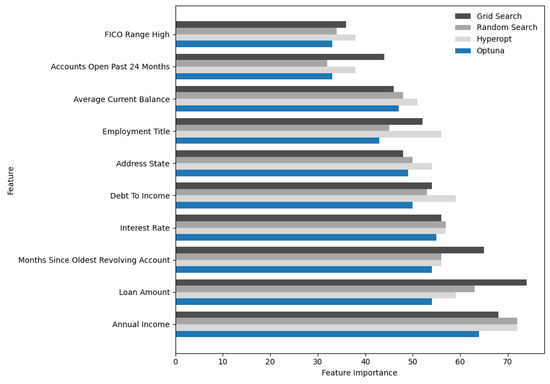
Figure 2.
Top-ten feature importance rankings based on the gain metric for LightGBM on the Lending Club dataset across four hyperparameter tuning methods (Grid Search, Random Search, Hyperopt, and Optuna).
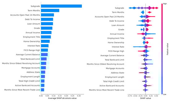

Figure 3.
SHAP feature importance rankings for LightGBM on the Lending Club dataset, optimized using the Grid Search (upper panel) and Random Search (lower panel) methods.

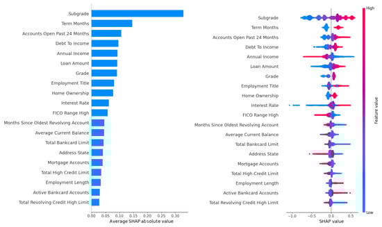
Figure 4.
SHAP feature importance rankings for LightGBM on the Lending Club dataset, optimized using the Hyperopt (upper panel) and Optuna (lower panel) methods.
Starting with Figure 2, which presents the top ten feature importance rankings based on the gain metric across all four tuning methods, the debt-to-income (DTI) ratio emerges as the most influential feature across Grid Search, Random Search, Hyperopt, and Optuna. The DTI ratio, which measures a borrower’s total debt obligations relative to their income, is a critical indicator of financial strain and repayment capacity, making its prominence unsurprising and consistent with domain knowledge in credit risk modeling. A high DTI ratio often signals increased default risk, as borrowers with substantial debt burdens relative to their income are less likely to meet repayment obligations. Following DTI, employment title consistently ranks as the second most important feature across all tuning methods. This feature captures socioeconomic factors, such as job stability and income potential, which are closely tied to creditworthiness. For instance, borrowers in higher-paying or more stable professions may exhibit lower default rates, while those in precarious or lower-income roles may face higher risks. Other consistently high-ranking features include loan amount, interest rate, and annual income, which appear among the top five across all methods. Loan amount and interest rate reflect the financial burden of the loan itself, with larger loans and higher interest rates often correlating with increased default probability due to greater repayment pressure. Annual income, on the other hand, provides insight into a borrower’s overall financial capacity, serving as a counterbalance to debt-related features. Additional features, such as credit history-related attributes (e.g., number of open accounts, recent credit inquiries) and loan-specific variables (e.g., term length), appear in the top ten, underscoring their role in assessing borrower reliability and loan risk. The remarkable consistency of these rankings across tuning methods is evidenced by a Spearman correlation coefficient exceeding , indicating that the choice of hyperparameter optimization method has minimal impact on the relative importance of features. This stability enhances LightGBM’s reliability for practical deployment in P2P lending, as it ensures that key risk drivers remain consistent regardless of the tuning approach, facilitating transparent and interpretable decision-making.
Figure 3 and Figure 4 provide a more granular perspective by presenting SHAP-based feature importance rankings for LightGBM. Figure 3 displays rankings optimized by Grid Search in the upper panel and Random Search in the lower panel, while Figure 4 displays rankings optimized by Hyperopt in the upper panel and Optuna in the lower panel. SHAP values, grounded in game theory, quantify each feature’s contribution to individual predictions, capturing complex interactions and offering a robust measure of interpretability. In Figure 3 (upper panel, Grid Search), the DTI ratio dominates, with a high SHAP value reflecting its substantial influence on model outputs, aligning with the gain-based findings and reinforcing DTI’s role as a primary driver of default risk. Employment title follows as the second most important feature, consistent with its high gain-based ranking, emphasizing its socioeconomic significance. In the lower panel (Random Search), DTI and employment title maintain their top positions, with similar rankings for loan amount, interest rate, and annual income, reflecting the stability of feature importance across these tuning methods. However, the prominence of employment title raises concerns about potential biases, as certain job titles may correlate with protected attributes such as race, gender, or socioeconomic status, which could lead to unfair lending decisions. For example, if job titles associated with lower-income or less stable professions disproportionately predict defaults, the model may inadvertently penalize borrowers from marginalized groups. Loan-specific features, including interest rate, loan amount, and term length, rank highly in Figure 3, consistent with their gain-based importance, as they directly influence the financial burden on borrowers. Annual income and credit history features, such as the number of open accounts and recent credit inquiries, also appear in the top ten, reflecting their role in assessing borrower stability and credit behavior. These features capture signals of financial distress, such as overextension through multiple credit lines or frequent credit applications, which are often precursors to default.
Figure 4, with Hyperopt in the upper panel and Optuna in the lower panel, shows nearly identical rankings to each other, with DTI and employment title maintaining their positions as the top two features in both panels. Interest rate and loan amount follow closely, underscoring their universal importance across tuning methods. Slight variations in SHAP values for lower-ranked features, such as credit inquiries, suggest minor differences in how Hyperopt’s and Optuna’s Bayesian optimization approaches prioritize feature interactions. For instance, Optuna may place slightly greater emphasis on credit history features due to its iterative sampling of promising hyperparameter configurations, which could influence how feature interactions are modeled. Nevertheless, the overall rankings in both panels remain highly correlated (Spearman correlation ), confirming the robustness of feature importance across Bayesian methods. The high consistency across Figure 3 and Figure 4 highlights the stability of LightGBM’s feature importance, regardless of the tuning method, which is critical for ensuring reliable and interpretable underwriting decisions in P2P lending platforms. The Spearman correlation coefficient exceeding across all methods reinforces this stability, suggesting that hyperparameter tuning variations do not significantly alter the model’s focus on key risk drivers.
A notable observation is the subtle difference between SHAP-based and gain-based rankings. While DTI and employment title remain the top features in both metrics, SHAP values in Figure 3 and Figure 4 place slightly greater emphasis on credit history features, such as the number of open accounts and recent credit inquiries, compared to the gain metric in Figure 2. This discrepancy arises because SHAP accounts for feature interactions and their impact on individual predictions, whereas the gain metric focuses on aggregate error reduction across tree splits. For example, credit inquiries may interact with loan amount or interest rate to signal financial distress, an effect that SHAP captures more explicitly by assigning higher importance to these interactions. In contrast, the gain metric prioritizes features that contribute most to overall error reduction, which may downplay interaction effects. This complementary nature of gain and SHAP metrics provides a comprehensive understanding of feature importance, with gain offering a high-level view of predictive power and SHAP providing nuanced insights into individual prediction contributions. The high correlation between rankings (Spearman ) across both metrics and all tuning methods further validates LightGBM’s interpretability, making it a reliable choice for P2P lending applications where transparency is essential for regulatory compliance and stakeholder trust.
The practical implications of these findings are significant for P2P lending platforms. Prioritizing features like DTI, loan amount, interest rate, and annual income in underwriting processes can enhance default prediction accuracy, as these factors directly relate to financial strain and repayment capacity. DTI, as the top-ranked feature across all methods in Figure 2, Figure 3 and Figure 4, is a straightforward indicator of a borrower’s ability to manage debt, making it a cornerstone of credit risk assessment. Loan amount and interest rate, which reflect the size and cost of the loan, are critical for evaluating repayment feasibility, while annual income provides a broader context for financial stability. Credit history features, such as open accounts and inquiries, offer additional signals of borrower behavior, helping platforms identify risky patterns like overextension or frequent borrowing. However, the high importance of employment title across all methods necessitates careful scrutiny. While it captures valuable socioeconomic signals, its use could introduce bias if certain job titles were disproportionately associated with specific demographic groups. For instance, if low-paying or unstable job titles correlate with higher default rates, the model may unfairly penalize borrowers from certain socioeconomic backgrounds, raising ethical concerns. This issue aligns with prior work emphasizing the need for fairness in credit scoring, as noted in the paper’s concluding remarks, which suggest complementing feature importance analysis with fairness audits using tools like SHAP to ensure ethical decision-making.
The stability of feature rankings across tuning methods and metrics enhances LightGBM’s suitability for scalable credit risk prediction. The computational efficiency of Bayesian methods (Hyperopt and Optuna), which achieve comparable feature importance stability to Grid Search with significantly reduced runtime (e.g., 3.19 vs. 241.47 min for LightGBM), further supports their practical deployment, as shown in the consistent rankings in Figure 4. This efficiency is particularly valuable for large datasets like Lending Club, where computational resources are a limiting factor. Moreover, the consistent identification of key risk drivers, such as DTI and employment title, enables platforms to develop transparent and interpretable models that align with regulatory requirements. However, the reliance on employment title underscores the need for further investigation into potential biases, as its prominence could inadvertently perpetuate inequities in lending decisions. Future research, as suggested in the paper, could explore feature interactions (e.g., DTI with annual income) to uncover nuanced risk patterns, potentially enhancing model performance and interpretability. Additionally, fairness-focused analyses, such as auditing employment title for correlations with protected attributes, could mitigate bias and ensure equitable credit scoring, aligning with the ethical considerations highlighted in the study’s conclusions.
The operational impact of implementing the feature importance findings from this analysis, namely, improved default prediction, increased investor satisfaction, platform retention, and compliance readiness, depends on several key factors. First, the quality and consistency of input data, such as accurate borrower financial information (e.g., DTI, annual income) and standardized employment title reporting, are critical to ensuring reliable model predictions in production. Second, the effective integration of the LightGBM model into P2P lending platforms requires robust infrastructure, including scalable computational resources and real-time data processing capabilities, to handle large datasets like Lending Club (233,015 records, 52 attributes). Third, addressing fairness concerns, particularly for features like employment title, necessitates ongoing fairness audits and bias mitigation strategies to align with regulations such as the EU AI Act and the U.S. Equal Credit Opportunity Act. Finally, stakeholder collaboration, including clear communication of model outputs to investors and regulators, is essential to translate transparency into trust and compliance. By addressing these factors, P2P lending platforms can maximize the practical benefits of this research, reducing default rates while enhancing investor confidence and regulatory alignment.
6. Conclusions
This study provides a comprehensive evaluation of hyperparameter tuning methods, Grid Search, Random Search, Hyperopt, and Optuna, for optimizing credit risk prediction models in peer-to-peer lending. By benchmarking Logistic Regression, Random Forest, XGBoost, and LightGBM across three real-world datasets (Lending Club, Australia, Taiwan), we assessed their predictive performance, computational efficiency, robustness, and interpretability, addressing the research questions outlined in Section 1.
LightGBM consistently outperformed other models, achieving the highest AUC (e.g., on Lending Club, on Australia, on Taiwan; Section 5.2, Table 5), driven by its efficient gradient-boosting framework (Section 4.2). XGBoost followed closely, while Random Forest and Logistic Regression showed lower discriminative power, particularly for imbalanced datasets. All tuning methods yielded comparable predictive performance, with AUC differences typically within 1–2% (Section 5.2), indicating multiple near-optimal hyperparameter configurations. The sensitivity analysis (Section 5.3) confirmed the robustness of these configurations, with perturbations in key hyperparameters resulting in minimal AUC changes (typically <0.4%) and high p-values (>0.05), ensuring reliable performance across tuning methods, particularly for Random Forest and LightGBM due to their variance-reducing and regularization mechanisms.
The feature importance analysis (Section 5.4) highlighted debt-to-income (DTI) ratio and employment title as critical drivers of default risk, with stable rankings across tuning methods (Spearman correlation ). The integration of SHAP-based rankings alongside the gain metric provided nuanced insights into feature interactions, emphasizing DTI’s role as a primary indicator of financial strain and employment title’s socioeconomic significance. However, the prominence of employment title raises fairness concerns, as it may correlate with protected attributes like race or socioeconomic status, necessitating fairness audits using tools like SHAP to ensure ethical decision-making. The operational impact of these findings depends on critical factors: high-quality input data (e.g., accurate DTI and standardized employment title reporting), scalable platform infrastructure for real-time model integration, ongoing fairness audits to mitigate biases, and stakeholder collaboration to ensure transparent communication with investors and regulators, aligning with standards like the EU AI Act and U.S. Equal Credit Opportunity Act.
These findings advocate the adoption of Bayesian optimization (Hyperopt, Optuna) in P2P lending platforms, balancing predictive accuracy with computational efficiency, as evidenced by up to -fold runtime reductions (e.g., vs. min for LightGBM on Lending Club; Section 5.2). LightGBM and XGBoost are recommended for their robust performance and scalability, particularly for large, imbalanced datasets like Lending Club (Table 1). Prioritizing features like DTI, loan amount, and interest rate in underwriting can enhance default prediction, reducing financial risk while supporting investor confidence and platform retention. The stability of feature rankings and hyperparameter configurations supports regulatory compliance by enabling transparent and interpretable decision-making.
While this study demonstrates the efficacy of HPO, it focused on a fixed set of hyperparameters and datasets. The reliance on random undersampling to address class imbalance (Section 4.1) may have discarded valuable data, potentially limiting model generalization. Future research could explore advanced resampling techniques (e.g., SMOTE variants) or cost-sensitive loss functions to better handle imbalanced classes, as suggested by prior work [41]. Extending the analysis to deep learning models [53,54,55] or stacking ensembles could further enhance predictive power, particularly for complex feature interactions. Investigating dynamic tuning strategies, such as adaptive iteration budgets, may optimize efficiency for smaller datasets like Australia. Additionally, analyzing feature interactions (e.g., DTI with annual income) could uncover nuanced risk patterns, improving model interpretability. Finally, evaluating models under real-world cost distributions with misclassification penalties would align predictions with financial objectives, while fairness-focused analyses could ensure equitable credit scoring.
This research underscores the value of efficient HPO methods and robust, interpretable models in credit risk modeling, offering P2P lending platforms scalable, transparent, and fair solutions for default prediction. By leveraging Bayesian optimization, ensemble models, and fairness-aware practices, practitioners can achieve near-optimal performance, reduce computational costs, and enhance financial inclusion while aligning with regulatory and ethical standards.
Author Contributions
Conceptualization, L.I.S. and A.R.H.; methodology, L.I.S. and A.R.H.; software, L.I.S. and A.R.H.; validation, L.I.S., A.R.H. and B.B.; formal analysis, L.I.S., A.R.H. and B.B.; investigation, L.I.S., A.R.H. and B.B.; resources, L.I.S., A.R.H. and B.B.; data curation, L.I.S.; writing—original draft preparation, L.I.S., J.M.O. and P.R.; writing—review and editing, L.I.S., J.M.O. and P.R.; visualization, L.I.S. and A.R.H.; supervision, B.B. All authors have read and agreed to the published version of the manuscript.
Funding
This research received no external funding.
Data Availability Statement
Three publicly available datasets were used in this study. Data can be found at https://www.lendingclub.com/, accessed on 12 November 2024, https://archive.ics.uci.edu/dataset/143/statlog+australian+credit+approval, accessed on 3 January 2025, and https://archive.ics.uci.edu/dataset/350/default+of+credit+card+clients, accessed on 3 January 2025.
Acknowledgments
The authors would like to express their sincere gratitude to the research laboratory “Applied Studies in Business and Management Sciences” at the Higher School of Commerce, Algeria, for their support and collaboration. They also extend their appreciation to Professor Mehdi Bouchetara for their insightful contributions to this work.
Conflicts of Interest
The authors declare no conflicts of interest.
Abbreviations
The following abbreviations are used in this paper:
| ANN | Artificial Neural Network |
| AUC | Area Under the ROC Curve |
| BN | Bayesian Network |
| BO | Bayesian Optimization |
| C | Inverse of Regularization Strength |
| CNN | Convolutional Neural Network |
| DT | Decision Tree |
| DTI | Debt-to-Income ratio |
| EI | Expected Improvement |
| ES | Evolution Strategies |
| FICO | Fair Isaac Corporation |
| GB | Gigabytes |
| GBDT | Gradient-Boosted Decision Tree |
| G-Mean | Geometric Mean |
| GS | Grid Search |
| HPO | Hyperparameter Optimization |
| LC | Lending Club |
| LDA | Linear Discriminant Analysis |
| LightGBM | Light Gradient-Boosting Machine |
| LIME | Local Interpretable Model-agnostic Explanations |
| LR | Logistic Regression |
| P2P | Peer-to-Peer |
| Probability Density Function | |
| RF | Random Forest |
| ROC | Receiver Operating Characteristic |
| RS | Random Search |
| SHAP | Shapley Additive Explanations |
| SMOTE | Synthetic Minority Oversampling Technique |
| SVM | Support Vector Machine |
| TPE | Tree-Structured Parzen Estimator |
| XAI | Explainable Artificial Intelligence |
| XGBoost | Extreme Gradient Boosting |
Appendix A
Table A1.
Performance metrics (in percentage) of machine learning models for credit risk prediction from Ko et al. [38].
Table A1.
Performance metrics (in percentage) of machine learning models for credit risk prediction from Ko et al. [38].
| LightGBM | CNN | LR | LDA | ANN | BC | RF | DT | |
|---|---|---|---|---|---|---|---|---|
| AUC | ||||||||
| Specificity | ||||||||
| Recall | ||||||||
| F-measure |
Table A2.
Performance metrics of machine learning models for credit risk prediction from Song et al. [15].
Table A2.
Performance metrics of machine learning models for credit risk prediction from Song et al. [15].
| Method | AUC | TPR | TNR | G-Mean | Accuracy |
|---|---|---|---|---|---|
| GBDT | |||||
| Random Forest | |||||
| AdaBoost | |||||
| Decision Tree | |||||
| Logistic Regression | |||||
| Multilayer Perceptron |
Table A3.
Performance metrics of machine learning models for credit risk prediction from Xia et al. [22].
Table A3.
Performance metrics of machine learning models for credit risk prediction from Xia et al. [22].
| Model | ACC (%) | Type I Error (%) | Type II Error (%) | AUC-H | Brier Score |
|---|---|---|---|---|---|
| AdaBoost | |||||
| AdaBoost-NN | |||||
| Bagging-DT | |||||
| Bagging-NN | |||||
| DT | |||||
| LR | |||||
| NN | |||||
| RF | |||||
| SVM | |||||
| GBDT | |||||
| XGBoost-MS | |||||
| XGBoost-GS | |||||
| XGBoost-RS | |||||
| XGBoost-TPE |
References
- Ma, B.-J.; Zhou, Z.-L.; Hu, F.-Y. Pricing mechanisms in the online peer-to-peer lending market. Electron. Commer. Res. Appl. 2017, 26, 119–130. [Google Scholar] [CrossRef]
- Lenz, R. Peer-to-peer lending: Opportunities and risks. Eur. J. Risk Regul. 2016, 7, 688–700. [Google Scholar] [CrossRef]
- Basha, S.A.; Elgammal, M.M.; Abuzayed, B.M. Online peer-to-peer lending: A review of the literature. Electron. Commer. Res. Appl. 2021, 48, 101069. [Google Scholar] [CrossRef]
- Ziegler, T.; Shneor, R.; Wenzlaff, K.; Wang, B.W.; Kim, J.; Odorovic, A.; Paes, F.F.; Suresh, K.; Zhang, B.Z.; Johanson, D.; et al. The Global Alternative Finance Market Benchmarking Report; University of Cambridge: Cambridge, UK, 2021. [Google Scholar]
- Ofir, M.; Tzang, I. An Empirical View of Peer-to-Peer (P2P) Lending Platforms. Berkeley Bus. Law J. 2022, 19, 175. [Google Scholar] [CrossRef]
- Bavoso, V. The promise and perils of alternative market-based finance: The case of P2P lending in the UK. J. Bank. Regul. 2020, 21, 395–409. [Google Scholar] [CrossRef]
- Song, P.; Chen, Y.; Zhou, Z.; Wu, H. Performance analysis of peer-to-peer online lending platforms in China. Sustainability 2018, 10, 2987. [Google Scholar] [CrossRef]
- Serrano-Cinca, C.; Gutiérrez-Nieto, B.; López-Palacios, L. Determinants of default in P2P lending. PLoS ONE 2015, 10, e0139427. [Google Scholar] [CrossRef]
- Lei, X. Discussion of the Risks and Risk Control of P2P in China. Mod. Econ. 2016, 7, 399–403. [Google Scholar] [CrossRef]
- Moscato, V.; Picariello, A.; Sperlì, G. A benchmark of machine learning approaches for credit score prediction. Expert Syst. Appl. 2021, 165, 113986. [Google Scholar] [CrossRef]
- Noriega, J.P.; Rivera, L.A.; Herrera, J.A. Machine Learning for Credit Risk Prediction: A Systematic Literature Review. Data 2023, 8, 169. [Google Scholar] [CrossRef]
- Lessmann, S.; Baesens, B.; Seow, H.-V.; Thomas, L.C. Benchmarking state-of-the-art classification algorithms for credit scoring: An update of research. Eur. J. Oper. Res. 2015, 247, 124–136. [Google Scholar] [CrossRef]
- Bischl, B.; Binder, M.; Lang, M.; Pielok, T.; Richter, J.; Coors, S.; Thomas, J.; Ullmann, T.; Becker, M.; Boulesteix, A.-L.; et al. Hyperparameter optimization: Foundations, algorithms, best practices, and open challenges. Wiley Interdiscip. Rev. Data Min. Knowl. Discov. 2023, 13, e1484. [Google Scholar] [CrossRef]
- Doshi-Velez, F.; Kim, B. Towards a rigorous science of interpretable machine learning. arXiv 2017, arXiv:1702.08608. [Google Scholar]
- Song, Y.; Wang, Y.; Ye, X.; Wang, D.; Yin, Y.; Wang, Y. Multi-view ensemble learning based on distance-to-model and adaptive clustering for imbalanced credit risk assessment in P2P lending. Inf. Sci. 2020, 525, 182–204. [Google Scholar] [CrossRef]
- Alam, T.M.; Shaukat, K.; Hameed, I.A.; Luo, S.; Sarwar, M.U.; Shabbir, S.; Li, J.; Khushi, M. An investigation of credit card default prediction in the imbalanced datasets. IEEE Access 2020, 8, 201173–201198. [Google Scholar] [CrossRef]
- Si, Z.; Niu, H.; Wang, W. Credit Risk Assessment by a Comparison Application of Two Boosting Algorithms. In Fuzzy Systems and Data Mining VIII; IOS Press: Amsterdam, The Netherlands, 2022; pp. 34–40. [Google Scholar]
- Komer, B.; Bergstra, J.; Eliasmith, C. Hyperopt-Sklearn: Automatic Hyperparameter Configuration for Scikit-Learn. In Proceedings of the 13th Python in Science Conference, Austin, TX, USA, 6–12 July 2014; van der Walt, S., Bergstra, J., Eds.; pp. 32–37. [Google Scholar]
- Akiba, T.; Sano, S.; Yanase, T.; Ohta, T.; Koyama, M. Optuna: A next-generation hyperparameter optimization framework. In Proceedings of the 25th ACM SIGKDD International Conference on Knowledge Discovery & Data Mining, Anchorage, AK, USA, 4–8 August 2019; pp. 2623–2631. [Google Scholar]
- Bergstra, J.; Bengio, Y. Random search for hyper-parameter optimization. J. Mach. Learn. Res. 2012, 13, 281–305. [Google Scholar]
- Stuke, A.; Rinke, P.; Todorović, M. Efficient hyperparameter tuning for kernel ridge regression with Bayesian optimization. Mach. Learn. Sci. Technol. 2021, 2, 035022. [Google Scholar] [CrossRef]
- Xia, Y.; Liu, C.; Li, Y.; Liu, N. A boosted decision tree approach using Bayesian hyper-parameter optimization for credit scoring. Expert Syst. Appl. 2017, 78, 225–241. [Google Scholar] [CrossRef]
- Cox, D.R. The regression analysis of binary sequences. J. R. Stat. Soc. Ser. (Methodol.) 1958, 20, 215–242. [Google Scholar] [CrossRef]
- Breiman, L. Random forests. Mach. Learn. 2001, 45, 5–32. [Google Scholar] [CrossRef]
- Chen, T.; Guestrin, C. XGBoost: A scalable tree boosting system. In Proceedings of the 22nd ACM SIGKDD International Conference on Knowledge Discovery and Data Mining, San Francisco, CA, USA, 13–17 August 2016; pp. 785–794. [Google Scholar]
- Ke, G.; Meng, Q.; Finley, T.; Wang, T.; Chen, W.; Ma, W.; Ye, Q.; Liu, T.-Y. LightGBM: A highly efficient gradient boosting decision tree. In Proceedings of the Advances in Neural Information Processing Systems, Long Beach, CA, USA, 4–9 December 2017; Volume 30. [Google Scholar]
- Nigmonov, A. Dataset from the US Peer-to-Peer Lending Platform with Macroeconomic Variables; Version 4; Mendeley Data: London, UK, 2021. [Google Scholar]
- Quinlan, R. Statlog (Australian Credit Approval); UCI Machine Learning Repository: Irvine, CA, USA, 1987. [Google Scholar]
- Yeh, I.-C. Default of Credit Card Clients; UCI Machine Learning Repository: Irvine, CA, USA, 2009. [Google Scholar]
- Malekipirbazari, M.; Aksakalli, V. Risk assessment in social lending via random forests. Expert Syst. Appl. 2015, 42, 4621–4631. [Google Scholar] [CrossRef]
- Emekter, R.; Tu, Y.; Jirasakuldech, B.; Lu, M. Evaluating credit risk and loan performance in online Peer-to-Peer (P2P) lending. Appl. Econ. 2015, 47, 54–70. [Google Scholar] [CrossRef]
- Namvar, A.; Siami, M.; Rabhi, F.; Naderpour, M. Credit risk prediction in an imbalanced social lending environment. Int. J. Comput. Intell. Syst. 2018, 11, 925–935. [Google Scholar] [CrossRef]
- Ramos, P.; Oliveira, J.M. Robust sales forecasting using deep learning with static and dynamic covariates. Appl. Syst. Innov. 2023, 6, 85. [Google Scholar] [CrossRef]
- Oliveira, J.M.; Ramos, P. Investigating the accuracy of autoregressive recurrent networks using hierarchical aggregation structure-based data partitioning. Big Data Cogn. Comput. 2023, 7, 100. [Google Scholar] [CrossRef]
- Oliveira, J.M.; Ramos, P. Cross-learning-based sales forecasting using deep learning via partial pooling from multi-level data. In Engineering Applications of Neural Networks; Iliadis, L., Maglogiannis, I., Alonso, S., Jayne, C., Pimenidis, E., Eds.; Springer Nature: Cham, Switzerland, 2023; pp. 279–290. [Google Scholar]
- Teply, P.; Polena, M. Best classification algorithms in peer-to-peer lending. N. Am. J. Econ. Financ. 2020, 51, 100904. [Google Scholar] [CrossRef]
- Ma, X.; Sha, J.; Wang, D.; Yu, Y.; Yang, Q.; Niu, X. Study on a prediction of P2P network loan default based on the machine learning LightGBM and XGboost algorithms according to different high dimensional data cleaning. Electron. Commer. Res. Appl. 2018, 31, 24–39. [Google Scholar] [CrossRef]
- Ko, P.-C.; Lin, P.-C.; Do, H.-T.; Huang, Y.-F. P2P lending default prediction based on AI and statistical models. Entropy 2022, 24, 801. [Google Scholar] [CrossRef]
- Rout, N.; Mishra, D.; Mallick, M.K. Handling imbalanced data: A survey. In International Proceedings on Advances in Soft Computing, Intelligent Systems and Applications: ASISA 2016; Springer: Berlin/Heidelberg, Germany, 2018; pp. 431–443. [Google Scholar]
- Veni, C.V.K.; Rani, T.S. On the classification of imbalanced datasets. Int. J. Comput. Sci. Technol. 2011, SP1, 145–148. [Google Scholar]
- Guo, H.; Li, Y.; Shang, J.; Gu, M.; Huang, Y.; Gong, B. Learning from class-imbalanced data: Review of methods and applications. Expert Syst. Appl. 2017, 73, 220–239. [Google Scholar]
- Huang, B.F.F.; Boutros, P.C. The parameter sensitivity of random forests. BMC Bioinform. 2016, 17, 331. [Google Scholar] [CrossRef]
- Bergstra, J.; Bardenet, R.; Bengio, Y.; Kégl, B. Algorithms for hyper-parameter optimization. In Proceedings of the 25th International Conference on Neural Information Processing Systems (NIPS’11), Granada, Spain, 12–15 December 2011; pp. 2546–2554. [Google Scholar]
- Snoek, J.; Larochelle, H.; Adams, R.P. Practical Bayesian optimization of machine learning algorithms. Adv. Neural Inf. Process. Syst. 2012, 25, 1–9. [Google Scholar]
- Chang, S.; Kim, S.D.; Kondo, G. Predicting default risk of lending club loans. CS229 Mach. Learn. 2015, 1–5. [Google Scholar]
- Jakka, G.M.; Panigrahi, A.; Pati, A.; Das, M.N.; Tripathy, J. A novel credit scoring system in financial institutions using artificial intelligence technology. J. Auton. Intell. 2023, 6, 824. [Google Scholar] [CrossRef]
- Friedman, J.H. Greedy function approximation: A gradient boosting machine. Ann. Stat. 2001, 29, 1189–1232. [Google Scholar] [CrossRef]
- Song, Y.; Li, Y.; Zou, Y.; Wang, R.; Liang, Y.; Xu, S.; He, Y.; Yu, X.; Wu, W. Synergizing multiple machine learning techniques and remote sensing for advanced landslide susceptibility assessment: A case study in the Three Gorges Reservoir Area. Environ. Earth Sci. 2024, 83, 227. [Google Scholar] [CrossRef]
- Amasyali, M.F. Improved space forest: A meta ensemble method. IEEE Trans. Cybern. 2018, 49, 816–826. [Google Scholar] [CrossRef]
- Abellán, J.; Castellano, J.G. A comparative study on base classifiers in ensemble methods for credit scoring. Expert Syst. Appl. 2017, 73, 1–10. [Google Scholar] [CrossRef]
- Melo, F. Area under the ROC Curve. In Encyclopedia of Systems Biology; Dubitzky, W., Wolkenhauer, O., Cho, K.-H., Yokota, H., Eds.; Springer: New York, NY, USA, 2013; pp. 38–39. [Google Scholar]
- Probst, P.; Boulesteix, A.-L.; Bischl, B. Tunability: Importance of hyperparameters of machine learning algorithms. J. Mach. Learn. Res. 2019, 20, 1–32. [Google Scholar]
- Oliveira, J.M.; Ramos, P. Evaluating the Effectiveness of Time Series Transformers for Demand Forecasting in Retail. Mathematics 2024, 12, 2728. [Google Scholar] [CrossRef]
- Teixeira, M.; Oliveira, J.M.; Ramos, P. Enhancing Hierarchical Sales Forecasting with Promotional Data: A Comparative Study Using ARIMA and Deep Neural Networks. Mach. Learn. Knowl. Extr. 2024, 6, 2659–2687. [Google Scholar] [CrossRef]
- Caetano, R.; Oliveira, J.M.; Ramos, P. Transformer-Based Models for Probabilistic Time Series Forecasting with Explanatory Variables. Mathematics 2025, 13, 814. [Google Scholar] [CrossRef]
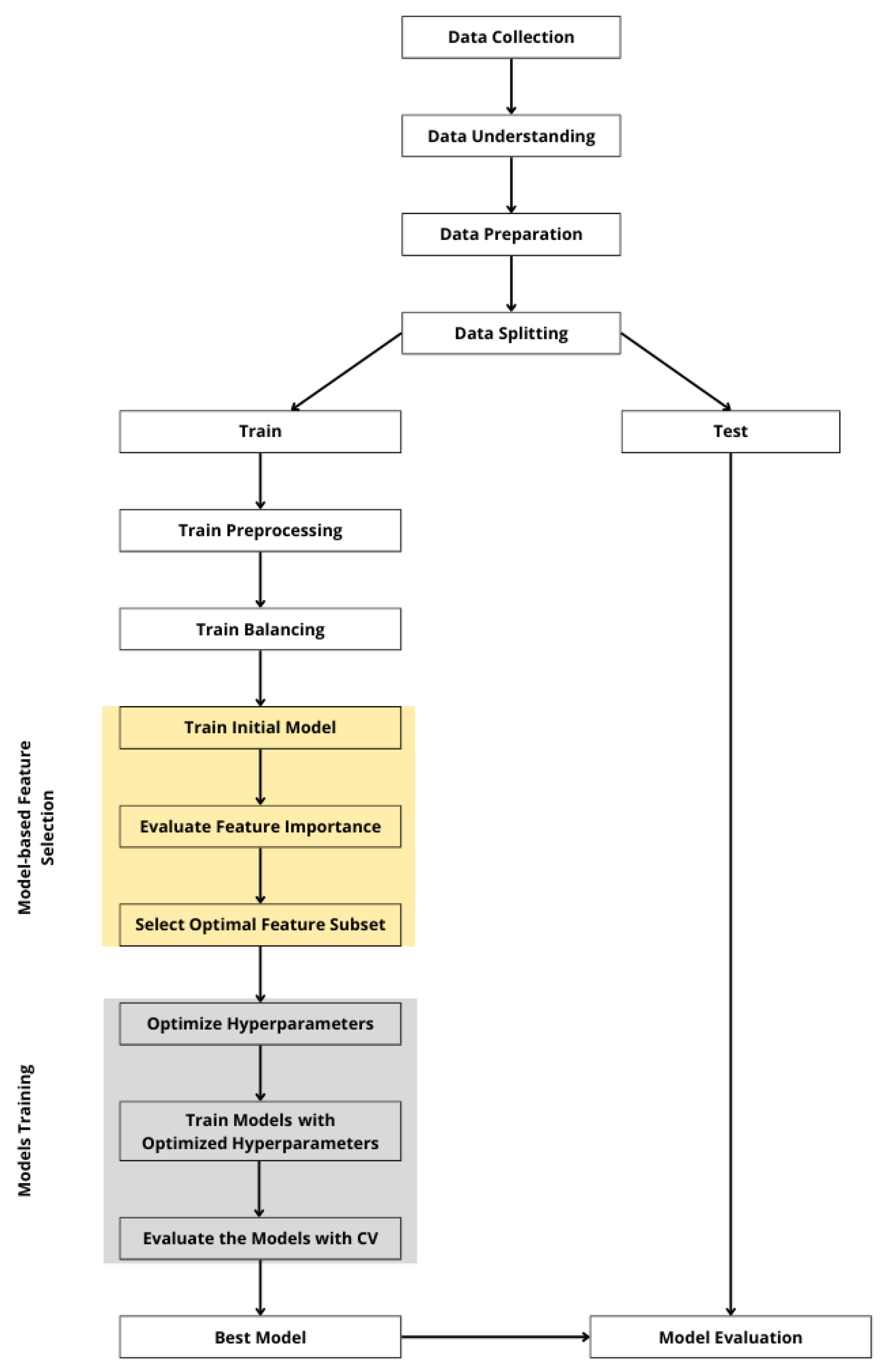

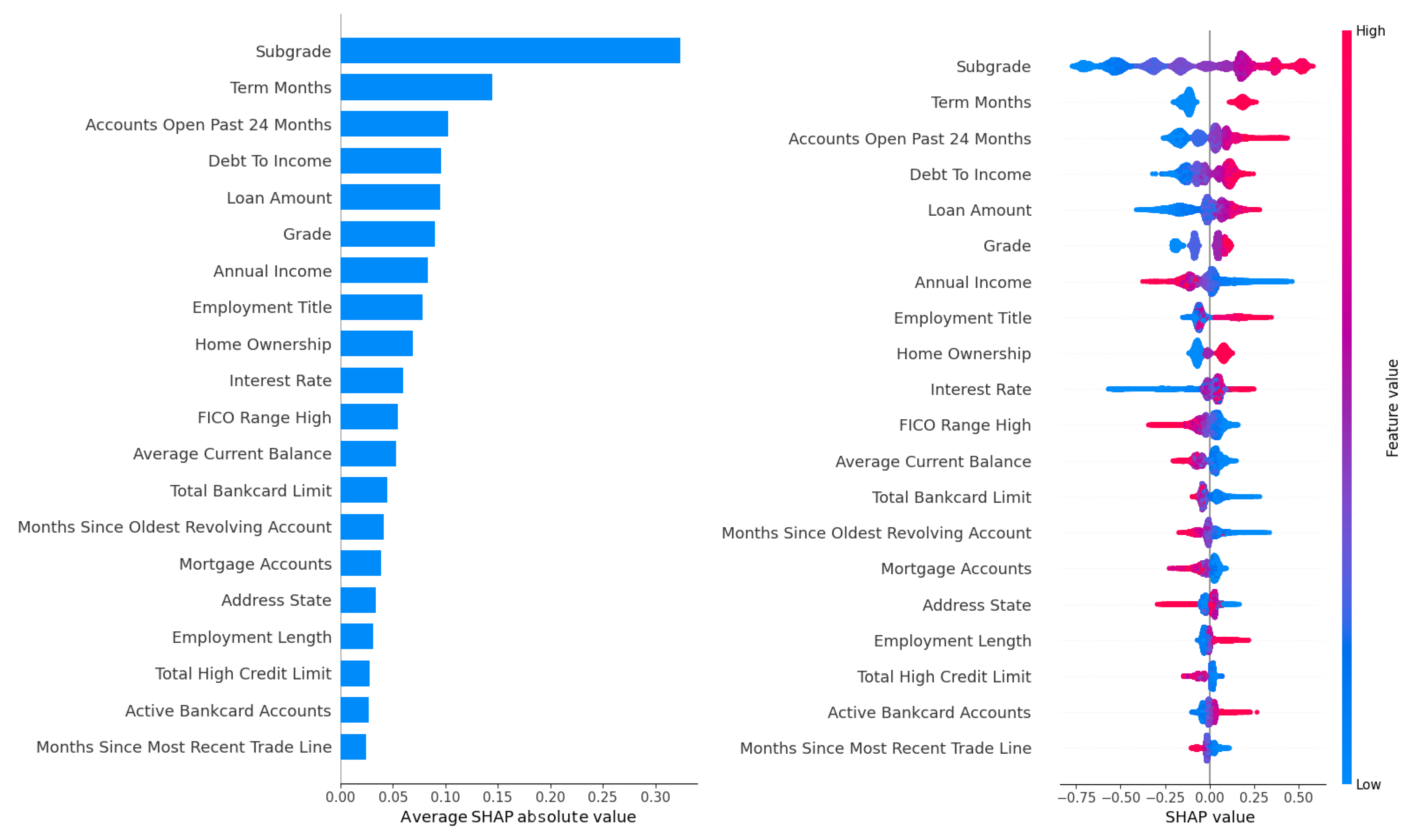
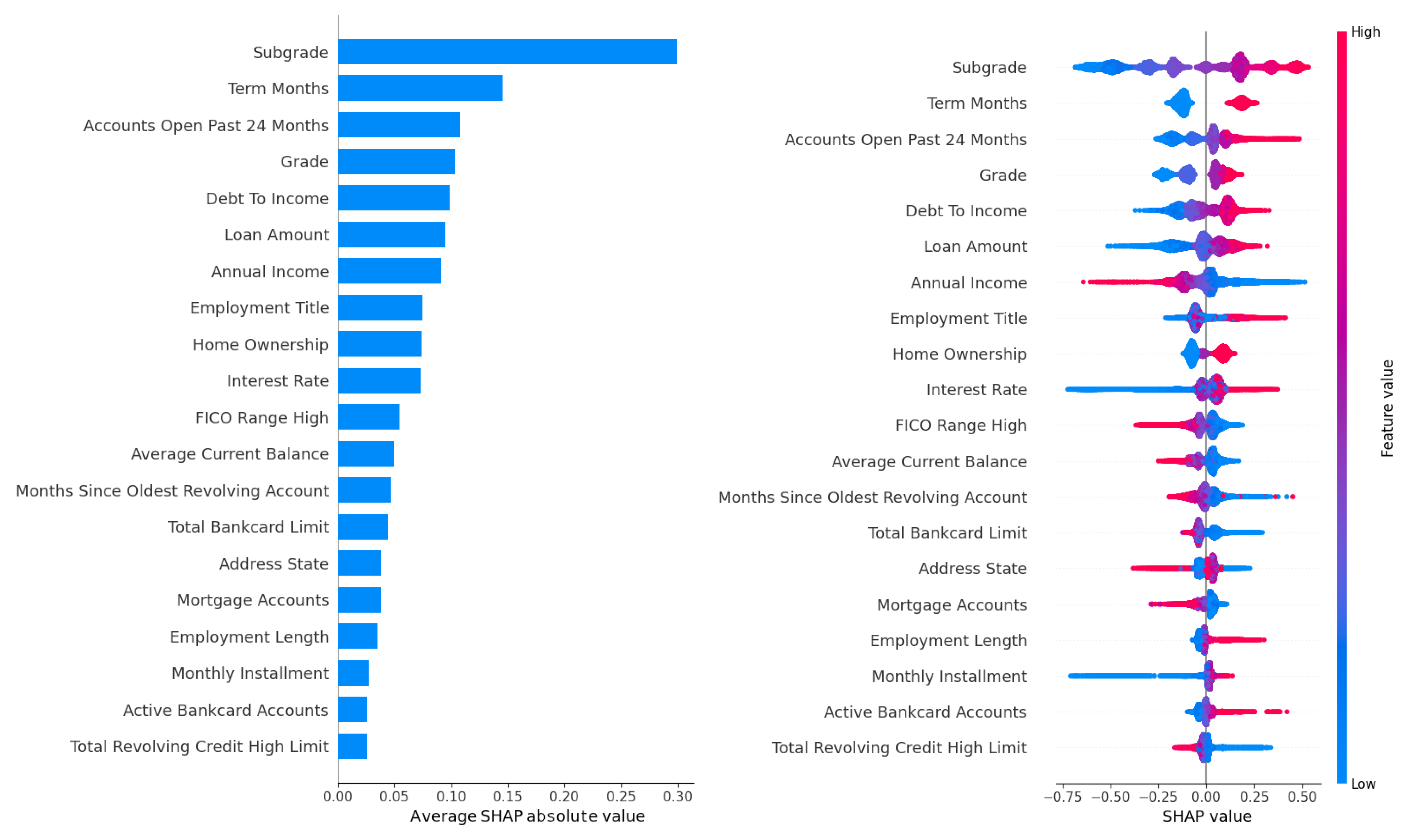
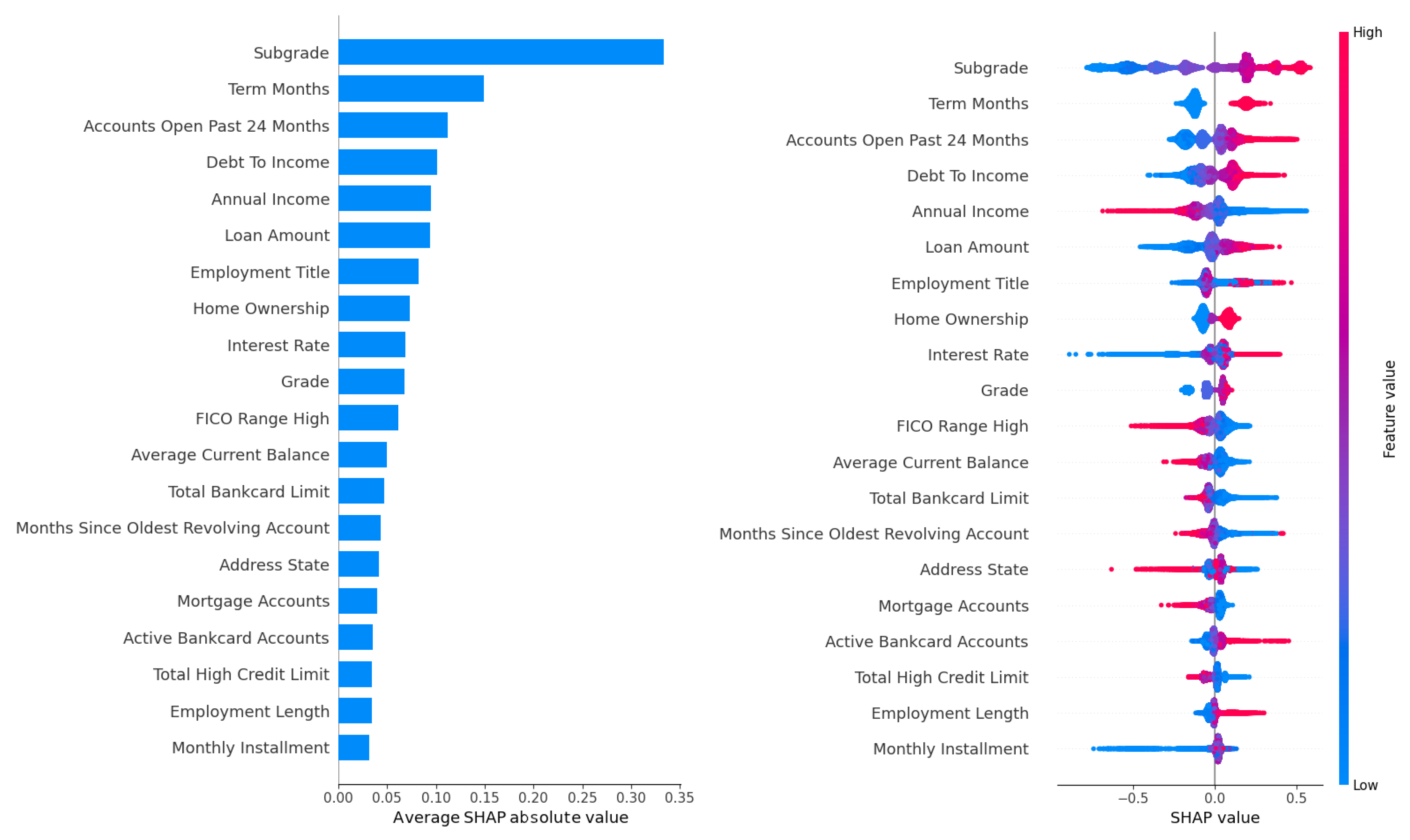
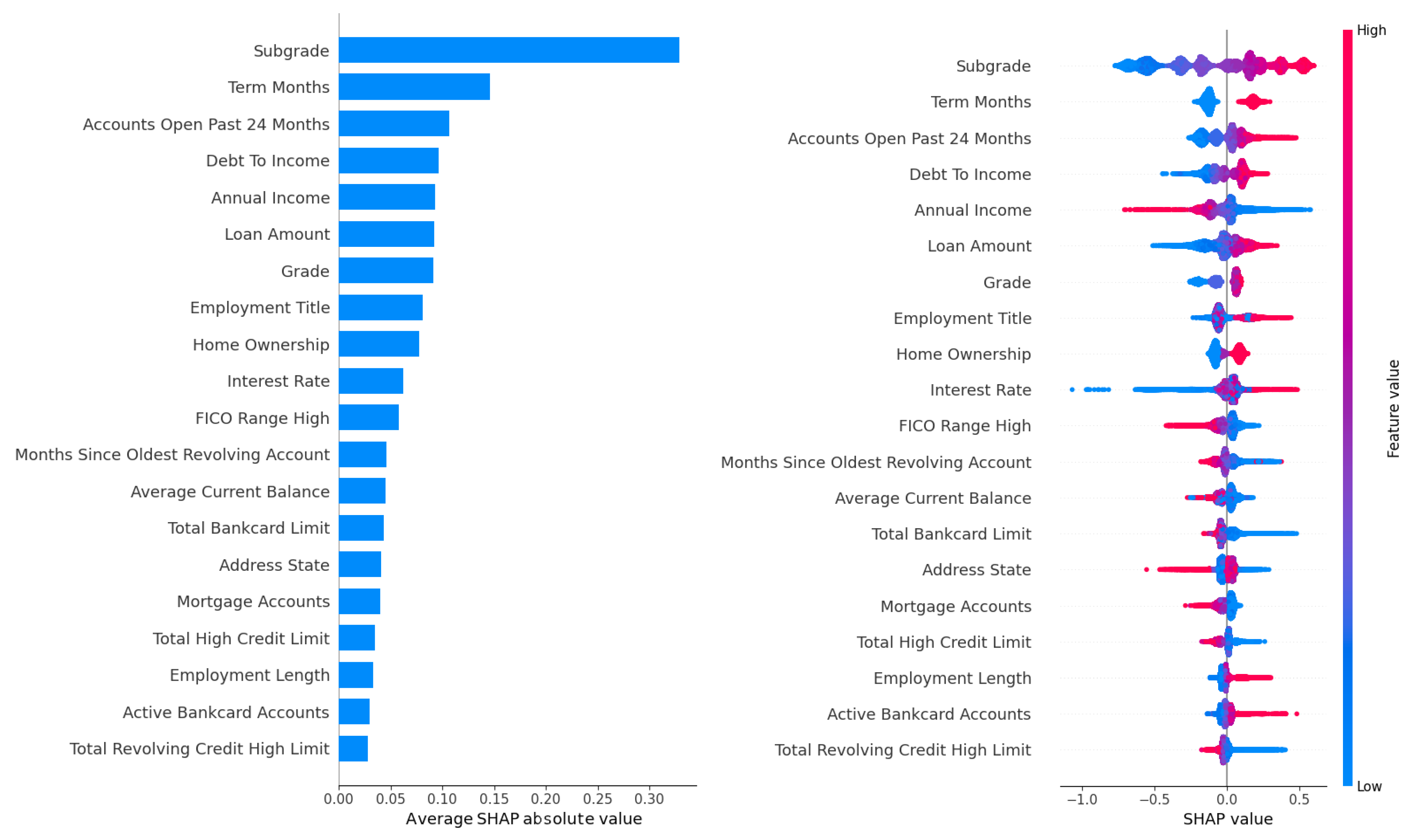
Disclaimer/Publisher’s Note: The statements, opinions and data contained in all publications are solely those of the individual author(s) and contributor(s) and not of MDPI and/or the editor(s). MDPI and/or the editor(s) disclaim responsibility for any injury to people or property resulting from any ideas, methods, instructions or products referred to in the content. |
© 2025 by the authors. Licensee MDPI, Basel, Switzerland. This article is an open access article distributed under the terms and conditions of the Creative Commons Attribution (CC BY) license (https://creativecommons.org/licenses/by/4.0/).