Abstract
The accurate short-term forecasting (PV) of power is crucial for grid stability control, energy trading optimization, and renewable energy integration in smart grids. However, PV generation is extremely variable and non-linear due to environmental fluctuations, which challenge the conventional forecasting models. This study proposes a hybrid deep learning architecture, Wavelet Transform–Transformer–Temporal Convolutional Network–Efficient Channel Attention Network–Gated Recurrent Unit (WT–Transformer–TCN–ECANet–GRU), to capture the overall temporal complexity of PV data through integrating signal decomposition, global attention, local convolutional features, and temporal memory. The model begins by employing the Wavelet Transform (WT) to decompose the raw PV time series into multi-frequency components, thereby enhancing feature extraction and denoising. Long-term temporal dependencies are captured in a Transformer encoder, and a Temporal Convolutional Network (TCN) detects local features. Features are then adaptively recalibrated by an Efficient Channel Attention (ECANet) module and passed to a Gated Recurrent Unit (GRU) for sequence modeling. Multiscale learning, attention-driven robust filtering, and efficient encoding of temporality are enabled with the modular pipeline. We validate the model on a real-world, high-resolution dataset of a Moroccan university building comprising 95,885 five-min PV generation records. The model yielded the lowest error metrics among benchmark architectures with an MAE of 209.36, RMSE of 616.53, and an R2 of 0.96884, outperforming LSTM, GRU, CNN-LSTM, and other hybrid deep learning models. These results suggest improved predictive accuracy and potential applicability for real-time grid operation integration, supporting applications such as energy dispatching, reserve management, and short-term load balancing.
1. Introduction
The accelerating global shift toward sustainable energy solutions has positioned photovoltaic (PV) systems at the heart of renewable power generation strategies. These systems have been driven by several factors, including minimal operating costs, environmental sustainability, and scalability across various applications that range from residential rooftops to large-scale solar farms. However, some limitations remain: the intermittency and non-linearity of PV generation are significantly influenced by strongly variable meteorological factors such as cloud cover, solar irradiance, temperature, and atmospheric pressure [1,2].
The accurate short-term forecasting of PV power generation is imperative for applications [3,4] like grid load management, reserve scheduling, energy trading, and real-time control in smart grids [5]. Traditional forecasting methods, such as physical models (e.g., numerical weather prediction, irradiance-based models) and statistical models (e.g., ARIMA, exponential smoothing), usually fail to capture the non-stationary, multiscale, and non-linear nature of PV data [1,6]. These models typically assume time-invariant relationships and linearity, which is less suitable for highly volatile and high-resolution solar data, especially during fast-changing weather transitions.
With the arrival of data-driven learning paradigms, deep learning (DL) models [7,8] are state-of-the-art time series forecasting tools due to their ability to learn implicit non-linear mappings directly from data [6]. In particular, Recurrent Neural Networks (RNNs) and their variants, such as Long Short-Term Memory (LSTM) [9] and Gated Recurrent Units (GRUs) [10], have been shown to provide improved performance in sequential dependency modeling. Convolutional Neural Networks (CNNs) [11] and Temporal Convolutional Networks (TCNs) [12] are better at extracting local temporal and spatial features and can be more efficiently trained. Nonetheless, standalone deep learning models, though powerful, are susceptible to the issues of overfitting, limitations in flexibility across temporal scales, and interpretability under complex real-world scenarios.
To address these limitations, current studies highlight the strength of hybrid deep learning models, which employ multiple learning processes and preprocessing techniques to identify both long-term trends and high-frequency fluctuations. These include the use of signal decomposition algorithms (i.e., Empirical Mode Decomposition (EMD) [13], Variational Mode Decomposition (VMD) [14], and Wavelet Transform (WT) [15]), which decompose the input signal into multiple frequency components and isolate meaningful features from noise. Similarly, attention mechanisms, particularly self-attention and channel attention modules like Efficient Channel Attention for Deep Convolutional Neural Networks (ECANet) [16], have proven highly effective in concentrating the model’s attention on the most relevant areas of the input signal, thereby improving both interpretability and accuracy.
However, despite these advances, there remains a research gap: many recent hybrid models do not combine multiresolution decomposition, attention-enhanced feature learning, and recurrent temporal modeling within a unified, end-to-end architecture. Additionally, such models often depend heavily on external meteorological inputs or complex preprocessing routines, which limit their portability and real-time deployment.
To address this gap, we propose a novel hybrid deep learning framework that integrates multiscale signal decomposition, global attention mechanisms, local temporal convolution, adaptive channel recalibration, and sequential memory encoding in a single pipeline for short-term PV forecasting. The full architectural design and evaluation procedures are detailed in the following sections.
The main objectives of this study are the following:
- Design an explainable and modular hybrid model that captures both global and local temporal dependencies in high-resolution PV data.
- Benchmark the proposed model against more than 18 architectures, including both external models and internal ablation variants.
- Demonstrate its applicability to real-time grid operations such as energy dispatching, reserve management, and short-term load balancing.
The rest of the paper is organized as follows:
1.1. Related Work
Recent advances in short-term PV prediction have focused on hybrid deep learning approaches that integrate signal decomposition, attention mechanisms, and sequential modeling. These studies aim to mitigate the natural volatility and non-stationarity of PV data through various architectural and preprocessing enhancements.
The authors of [16] proposed a physics-constrained deep learning model incorporating Complete Ensemble Empirical Mode Decomposition with Adaptive Noise (CEEMDAN) and CNN-LSTM with a novel physics-aware loss function that penalizes physically unreasonable results, such as negative predictions during non-generation periods. Their model demonstrated improved accuracy and robustness under adverse weather conditions from real PV datasets. However, its use of external meteorology inputs and a pre-specified decomposition pipeline may limit scalability across different geographies and PV installations.
A CEEMDAN–Informer hybrid model was also introduced in [17] for PV prediction in hourly steps with the use of CEEMDAN for reducing non-stationarity dimensions and the Informer transformer for sparse long-sequence modeling. Their model achieved remarkable accuracy gains with the MAE and RMSE reduced up to 37.5% and 34.74%, respectively, over regular LSTM, GRU, and Transformer models. Nevertheless, its high-resolution meteorological feature reliance restricts it to ultra-short-term or sensor-limited scenarios.
In [18] the authors introduced CGaformer, a CNN1D model supported by Global Additive Attention (GADAttention) and Auto-Correlation mechanisms for efficient long-range temporal learning. CGaformer attains state-of-the-art forecasting performance as well as computational efficiency while maintaining architectural complexity; nevertheless, it continues to depend on exogenous weather data for optimal performance.
A multi-stage hybrid approach was presented in [19], combining Isolation Forest (IF) for outlier removal, Non-linear Probabilistic CNN (NPCNN) for feature extraction, and Wavelet-KNN for reducing variance post-prediction. Applied to a national PV demonstration dataset, the model reduced the MAE and RMSE by approximately 14.3% and 13.1% compared to LSTM. However, the layered architecture involves inference latency and implementation complexity.
The authors of [20] proposed DSEHM, a dynamic selective ensemble of AttnGRU, Informer, TCN, and XGBoost, with scenario-adaptive weighting according to irradiance and temporal variability. The DSEHM tested on smart grid data reduced the MAE by 22.55% and RMSE by 19.01% but at the cost of coordination and computational overhead.
The authors of [21] developed MHA-BiLSTM-CNN, a two-stream hybrid framework using a CNN for local pattern extraction and BiLSTM for modeling long dependencies. MHA-based fusion enhanced explainability and reduced the MAE by 21.4% compared to baselines. The model is sensitive to the hyperparameter tuning of many modules and needs short input sequence adaptation.
EDCPSO-MQLSTM was proposed in [22], a probabilistic forecasting model with Multi-Quantile LSTM and Evolutive Distributed Chaotic Particle Swarm Optimization. The model is aimed at ultra-short-term prediction with high Prediction Interval Coverage Probability (PICP of 94.2%) and improved pinball loss, but it introduces high computational burdens due to optimization. This highlights the growing importance of uncertainty-aware forecasting approaches in ultra-short-term PV prediction.
A recent contribution in [23] explored MIC-WSO-TCN, a hybrid architecture incorporating the Maximal Information Coefficient (MIC) for feature selection, White Shark Optimizer (WSO) for hyperparameter tuning, and a TCN for temporal learning. Although achieving MAE and RMSE reductions of up to 38.1% and 29.9%, respectively, the model’s dependence on accurate meteorological inputs and metaheuristic tuning increases its operational complexity.
The authors of [13] proposed EMD–GRU–Attention (EGA), a Kalman denoising, Empirical Mode Decomposition, and attention-augmented GRU deep learning model for solar radiation forecasting. EGA achieved 17.94% and 15.2% RMSE and MAE gains, respectively, but suffered from high preprocessing requirements and persistent input signal assumption.
Complementing these efforts, Reference [24] reported a TCN–ECANet–GRU hybrid that embeds Efficient Channel Attention within TCN residual blocks prior to a GRU sequencer. Trained on 5 min multivariate PV/meteorological measurements from a real plant, the model achieved season-best normalized errors (e.g., RMSE = 0.0195; MAE = 0.0128; R2 ≈ 0.997 in winter) and consistently outperformed SVR, GRU, TCN, CNN-GRU, and TCN-GRU across single- and multi-step horizons. The findings highlight the utility of channel recalibration before gated recurrence; limitations include reliance on exogenous meteorological inputs, single-site/single-year evaluation, and occasional non-physical evening outputs, which may constrain generalization under sensor outages or across geographies.
In parallel, Transformer–GRU hybrids have been explored for PV and irradiance forecasting and, more broadly, for long-horizon sequence learning. Reference [25] introduced a GRU–Temporal Fusion Transformer with a DILATE loss that achieved MAE = 1.19, MSE = 2.08, and RMSE = 1.44 on the “Daily Power Production of Solar Panels” dataset, with Diebold–Mariano tests (p < 0.05) confirming significant gains over XGBoost, N-HiTS, and N-BEATS. Reference [26] presented a transformer-infused recurrent architecture (attention-augmented BiLSTM encoder with a GRU decoder) reaching R2 = 0.9983, RMSE = 0.0140, and MAE = 0.0092 on solar irradiance data, outperforming the ANN, GRU, BiLSTM, BiLSTM–GRU, and vanilla Transformer. These findings indicate that combining global self-attention with lightweight gated recurrence captures complementary dependencies more effectively than purely recurrent or purely transformer models; the remaining limitations include sensitivity to sequence length and the need for careful feature engineering or exogenous inputs when transferring across sites and horizons.
While these works contribute substantially to the field, they often suffer from one or more of the following drawbacks: reliance on exogenous meteorological data, non-modular and complex architectures, and the absence of a unified mechanism that can capture global, local, and multiscale temporal features in an end-to-end manner.
The proposed WT–Transformer–TCN–ECANet–GRU model builds on prior work via the following:
It is meteorology-independent, reducing reliance on exogenous weather sensors.
It combines wavelet decomposition, self-attention, local convolution, and recurrent memory in a unified pipeline, allowing for comprehensive multiscale feature extraction and learning.
Its modularity improves interpretability, scalability, and training efficiency, especially under high-frequency PV data conditions.
This study aims to improve upon existing methods by enhancing accuracy and robustness and also address real-world deployment feasibility for smart grid forecasting tasks. This architecture offers a practical and unified response to the challenges repeatedly identified in the recent literature.
1.2. Proposed Hybrid Model: WT–Transformer–TCN–ECANet–GRU
WT–Transformer–TCN–ECANet–GRU is a novel hybrid deep architecture specifically designed for PV power forecasting. The proposed model integrates multiple modeling paradigms (frequency domain analysis, attention mechanisms, and sequential learning) to capture global and local temporal dependences in time series data effectively. The proposed architecture is composed of a structured pipeline of specialized modules, each module being specifically designed to extract, transform, and cleanse temporal features of high fidelity.
As illustrated in Figure 1, the model processes input data with the following components, each designed to handle a particular level of temporal abstraction:
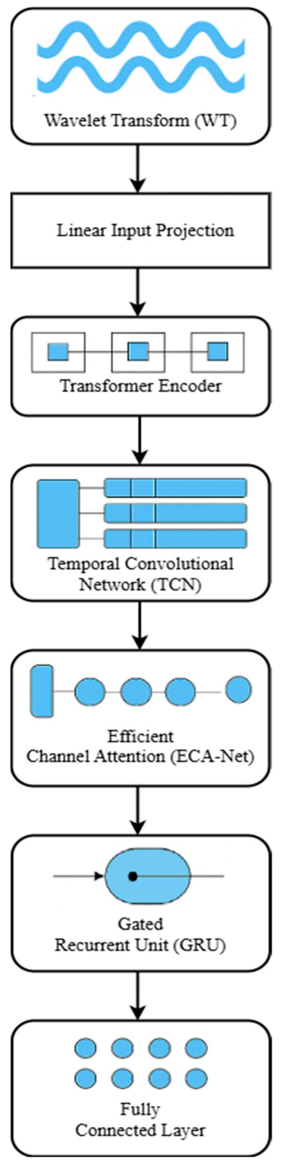
Figure 1.
WT–Transformer–TCN–ECANet–GRU model architecture.
- Wavelet Transform (WT).
- Linear Input Projection.
- Transformer Encoder.
- Temporal Convolutional Network (TCN).
- Efficient Channel Attention (ECANet).
- Gated Recurrent Unit (GRU).
- Fully Connected (FC) Layer.
Their combination allows the architecture to effectively extract multiscale patterns, long-term relationships, and essential temporal features, crucial to high-quality PV forecasting, as detailed below.
The end-to-end architecture is mathematically defined as follows:
where
- Xt: Multivariate input time series at t.
- ŷt: PV power predicted value.
- fWT(Xt): WT extracting time–frequency components.
- fProj: Linear projection mapping the decomposed signal into a common latent space.
- fTrans: Transformer encoder capturing global long-range dependencies.
- fTCN: TCN for local and mid-term features.
- fECA: ECANet model that emphasizes informative features.
- fGRU: GRU encoding sequential temporal dependencies.
- : Fully connected output layer producing final prediction.
Wavelet Transform (WT): The proposed architecture starts with a wavelet transformation of the input time series, which decomposes the signal into multiple frequency sub-bands. Using the wavelet’s ability to perform multiscale time–frequency analysis allows the model to capture both long-term trends and short-term fluctuations in the data. By transforming the raw time series into a set of approximation and detail coefficients (at different resolution levels) [27], the WT block provides an insightful representation of the input that isolates disparate temporal dynamics [15].
Mathematically,
where
- Aj denotes the approximation coefficients at level j of the wavelet decomposition.
- Dj: The detail coefficients at level j of the wavelet decomposition.
The wavelet decomposition multiresolution output is then forwarded to the subsequent projection layer, which ensures that downstream modules can use these extracted features.
A linear input projection layer (a fully connected mapping) then converts the wavelet-transformed features to the appropriate dimension for the Transformer encoder. Like an embedding layer, it takes the multiscale coefficients output from the WT stage and maps them into a dimensional feature space that can be input to attention-based encoding. This transformation is expressed as follows:
where
- Zt represents the projected input features.
- Wp and bp are the weight matrix and bias of the projection layer, respectively.
Like an embedding layer, it takes the multiscale coefficients output from the WT stage and maps them into a dimensional feature space suitable for attention-based encoding. Consequently, this operation ensures that all time steps and sub-sequences are mapped as vectors in a common latent space such that the attention mechanism can effectively coordinate with all features. The projected features (typically with positional encoding added in practice) are used as input to the Transformer encoder.
Transformer Encoder: The predicted time series features are then passed through a Transformer encoder module, which has been designed to learn long-range dependencies through self-attention mechanisms [28,29].
The process starts with the initialization of the hidden representation at the first layer with the projected input:
Then, each subsequent layer (for l = 1,…,L) updates the representation using the following:
- MSA executes scaled dot-product attention across multiple heads to enable the model to attend to different positions in the sequence.
- FFN is typically a two-layer feed-forward network with ReLU activation at each time step independently.
This formulation provides context for each position in the input sequence by considering its relationship to all other positions using attention and then refines it through a non-linear transformation.
The multi-head self-attention sub-layer allows the model to capture patterns in the entire sequence simultaneously and capture global temporal relationships (e.g., seasonality or long trends) without recurrence. Attention-based encoding eliminates the vanishing gradient and memory bottleneck of traditional RNNs by enabling direct interaction between distant time steps [29]. The Transformer encoder thus produces a richer representation of the input sequence, endowing it with both content and long-range context of the time series. The output is then passed to the TCN module for further temporal feature extraction.
Temporal Convolutional Network (TCN): The TCN module is included to obtain local and medium-term temporal patterns not necessarily in an explicit manner, learned by the global attention of the Transformer [23]. A TCN consists of multiple layers of dilated causal one-dimensional convolutions, and the output of every layer has the same length as the input. Each layer in the TCN processes its input by updating an internal hidden state representation, which evolves hierarchically through the stacked convolutional layers.
The hidden state at layer l is calculated through 1D causal convolution as follows:
where
- Wl and bl are, respectively, the weight and bias parameters of layer l.
- ReLU: The activation function.
This formulation enables an exponentially large receptive field while preserving the chronological order of information. In practical application, dilated causal convolutions allow the TCN to learn short-to-mid-range dependencies and recurring patterns (e.g., spikes or seasonality at an integer interval) that complement the Transformer’s capabilities. With the support of a stacked TCN and residual connections coupled with appropriate dilation factors, hierarchical temporal features are extracted from the Transformer’s output, and these local trends and high-frequency pattern representations are thereafter forwarded to the attention module for refinement.
Efficient Channel Attention (ECANet): After the TCN, an adaptive channel attention mechanism (ECA) is employed to adaptively recalibrate the channel-wise features. Specifically, following an adaptive average pooling of the TCN output, a small convolution (with kernel size k) is utilized to obtain local cross-channel interactions and produce an attention weight for each feature channel. The kernel size k is adaptively determined as a function of the number of channels, by ensuring that the attention mechanism is specifically engineered following the feature dimensionality [30]. This approach significantly reduces complexity compared to a standard Squeeze-and-Excitation module or Convolutional Block Attention Module (CBAM) while effectively highlighting the most informative channels. The ECA module adds only k trainable parameters but sacrifices little performance compared to heavier attention blocks. By focusing the TCN output channels according to their importance, ECANet allows the model to concentrate on important features (e.g., emphasize specific frequency bands or strongly predictive sensors) and suppress less critical information. The attention-weighted feature sequence is input into the GRU layer.
Channel-wise attention weight computation:
Attention-weighted output:
where
- σ: The sigmoid activation function.
- Conv1D: A one-dimensional convolution.
- AvgPool: Channel-wise average pooling.
- is the output feature map from the TCN module.
- ⊙: The element-wise (Hadamard) product.
- : The learned channel-wise attention scores.
- : The reweighted feature map passed to the GRU layer.
Gated Recurrent Unit (GRU): The GRU layer is added to capture any remaining sequential dependencies and to integrate the information over time using gating mechanisms. In this architecture, the GRU takes the feature sequence (augmented with ECA) as input and processes it step by step, maintaining a hidden internal state [31]. The gating mechanism’s structure enables any GRU to learn to keep long-term information or discard it as needed while modeling complex temporal dynamics and noise in the time series. Compared to standard LSTMs [32], GRUs require fewer parameters (since there is no extra output gate) but often have equivalent performance. This makes the GRU an attractive, computationally inexpensive choice for adding a recurrent inductive bias on top of the attention and convolutional representations.
The internal computations of the GRU are defined as follows:
Update gate: This gate controls how much of the previous hidden state should be retained.
where
- : The previous hidden state.
- σ: The sigmoid activation function.
- and : The trainable weights for the input and hidden state, respectively.
- : The input at time step t.
The reset gate determines how much past information to forget when computing the new memory content.
- and are reset gate weights.
Candidate hidden state: The proposed new memory content, influenced by the reset gate.
- ⊙ denotes element-wise multiplication.
- tanh: The hyperbolic tangent activation function.
- : The weight matrices for the candidate update.
Final hidden state update: A linear interpolation between the previous hidden state and the new candidate, controlled by the update gate.
The GRU output (e.g., the final hidden state or sequence of states, based on the task) is a concise summary of the time series that is informed by both long-term contexts and recent observations.
Fully Connected Layer: The last component of the model is a fully connected output layer that projects the GRU representation to the target prediction. This layer (essentially, a linear combination of the GRU output features) produces the prediction or classification output in the desired form. The linear output layer architecture keeps the end-to-end model differentiable and allows the training of earlier layers (WT to GRU) to optimize prediction accuracy. The final model output is obtained by linearly projecting the current hidden state output weights and bias.
- The weight matrix of the output.
- : The output bias.
- : The forecasted output at time t.
In summary, the WT–Transformer–TCN–ECANet–GRU architecture integrates powerful modules—wavelet-based decomposition for multiscale feature extraction, self-attention for capturing long-range dependency, convolution for learning local patterns, channel attention for weighing feature importance, and gated recurrence for sequential inference—into a single, end-to-end pipeline aimed at capturing every facet of temporal dynamics in the data. Each component addresses a specific aspect of the time series learning problem, and together they contribute to robust predictive performance.
1.3. Novelty and Distinction from Other Hierarchical Hybrid Architectures
While several hybrid forecasting models adopt hierarchical flows (e.g., Transformer–GRU, TCN–GRU–ECA Net, CNN–LSTM), the proposed WT–Transformer–TCN–ECA Net–GRU implements a hierarchical and interdependent feature processing flow that differs both structurally and functionally from prior work [24,26].
Structural Novelty: In typical hierarchical architectures, modules follow a linear, feed-forward sequence with each block processing on the output of its predecessor in full isolation. Representative cases are the following: Transformer–GRU [25], where global attention is taken before sequential modeling but where the explicit extraction of local patterns or recalibration of channels is skipped; TCN–GRU–ECANet [24], where local channel modeling and attention are skipped but where global context and multiresolution frequency features are also not taken into account; and CNN–LSTM [16], where spatial/feature extraction and recurrent modeling coexist but where frequency decomposition or attention mechanisms are not explicitly combined. By contrast, our model embeds multiresolution wavelet decomposition inside the learnable stack rather than as a fixed pre-step. The WT coefficients are linearly projected into a shared latent space and then passed to the Transformer, enabling decomposed representations to interact with downstream modules—Transformer (global dependencies), TCN (local temporal patterns), ECA Net (channel recalibration), and GRU (sequential memory)—within one trainable graph.
Functional Interdependence: Transformer outputs (global context) condition the subsequent TCN stage (local features); ECA Net then recalibrates channels before the GRU integrates a calibrated multiscale sequence rather than raw features. This global-to-local conditioning pathway ensures that each stage operates on contextually enriched inputs, unlike the baselines above, where modules are connected serially but not mutually informed. Baselines such as Transformer–GRU, TCN–GRU–ECA Net, and CNN–LSTM lack either the multiresolution decomposition, the explicit global-to-local conditioning, or the inter-stage channel recalibration, resulting in weaker coupling between hierarchical stages.
Figure 2 compares the proposed WT–Transformer–TCN–ECA Net–GRU with three representative baselines to illustrate structural and functional differences. All diagrams use a consistent visual grammar (block shapes and arrows) for fair comparison.
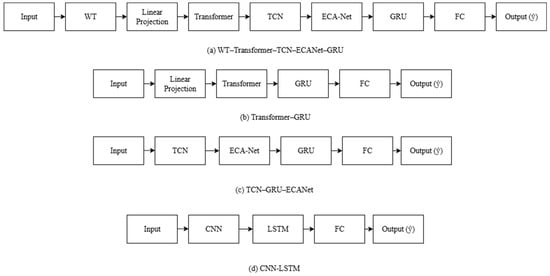
Figure 2.
Comparative diagram of hierarchical processing flows.
Figure 2a: Proposed WT–Transformer–TCN–ECA Net–GRU: Input → WT → Linear Projection → Transformer → TCN → ECA Net → GRU → FC → Output (ŷ). The WT’s outputs are projected to a shared latent space and fused with Transformer features before local extraction. ECA Net performs channel-wise recalibration before the GRU, ensuring memory integrates a selectively emphasized representation.
Figure 2b: Transformer–GRU baseline: Input → Linear Projection → Transformer → GRU → FC → Output (ŷ). This captures long-range dependencies but lacks the WT and TCN/ECA Net; the GRU receives sequence-level attention features without explicit multiscale/local refinement.
Figure 2c: TCN–GRU–ECA Net baseline: Input → TCN → ECA Net → GRU → FC → Output (ŷ). This models local patterns and applies channel recalibration but omits global attention and frequency domain decomposition; long-range dependencies are implicit.
Figure 2d: CNN–LSTM baseline: Input → CNN → LSTM → FC → Output (ŷ). This learns local spatial/temporal patterns and sequential dependencies but omits frequency decomposition, explicit attention mechanisms, and global-to-local feature conditioning.
The proposed pipeline is not a mere reordering of blocks; it integrates decomposition (WT), global attention (Transformer), local convolution (TCN), channel attention (ECA Net), and recurrent memory (GRU) into a single, coupled hierarchy in which later stages consume context-conditioned and channel reweighted features. This is supported by the ablation study results (Section 3.1.2), where relocating or removing modules consistently causes statistically significant performance degradation, reinforcing that the novelty lies in hierarchical interdependence rather than arbitrary block permutation.
2. Materials and Methods
Based on this rich and high-resolution dataset, we developed a novel hybrid forecasting model to capture both global and local temporal features. The model architecture is detailed below.
2.1. Dataset Description
This study uses a full dataset of photovoltaic (PV) panel production in the presidential building of Ibn Tofail University in Kenitra, Morocco. The data span one year, from 1 January 2022 to 31 December 2022, and consist of measurements taken every five min. There are 95,885 records in the dataset.
Each input contains the following:
- Timestamp: The date and time of the measurement with a five-min step.
- Production (Watt-hours): The solar energy produced by the PV panels of the building.
To better understand the dataset’s behavior, Figure 3 presents the average daily PV production pattern, showing the typical diurnal shape with zero values during nighttime and a single production peak around midday.
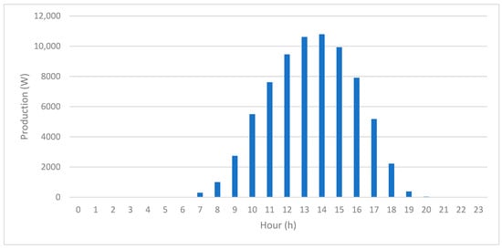
Figure 3.
Daily average PV production profile.
Key statistics of the dataset include the following:
- Mean production: ~3281 Wh; median: ~2742 Wh.
- Minimum value: 0 Wh in nighttime hours; maximum: 18,044 Wh in peak sunlight.
- Standard deviation: ~3419 Wh.
These statistics confirm the strong intraday variability in and skewness of PV production, characteristic of solar irradiance-driven systems.
Before modeling, basic preprocessing steps were applied:
- Missing Data Handling: Bad or missing measurements were interpolated or removed to maintain the continuity of the time series.
- Normalization: The PV power values were normalized using RobustScaler before being input to the neural networks, which scales the PV data by removing the median and dividing by the interquartile range. This approach is robust to outliers and helps stabilize deep learning model training.
- Train–Test Split: Among the traditional approaches used for time series is the technique employing the initial part of the timeline for training and the most recent part for the test, such that test data temporally succeeds training data to mimic actual forecasting; 70% of the dataset in this study is used for training, and 30% is reserved for testing.
2.2. Hyperparameters
One set of hyperparameters was adopted to train them and provide a consistent and fair comparison of all models. The models used a sequence length of 64 and a hidden size of 64 for both recurrent and convolutional modules. The Transformer had an embedding dimension (d_model) of 64, 4 attention heads, and 2 encoder layers, while TCNs had a 3-sized kernel for spatial–temporal feature extraction, and the GRU and LSTM recurrent modeling architectures were fixed to one-layer mode, operating in batch-first order.
Data preprocessing was standardized for all experiments with the RobustScaler. For signal decomposition, CWT was chosen with the Morlet wavelet because of its favorable time–frequency localization properties and effectiveness in modeling irradiance signals characterized by smooth oscillatory patterns. Scale widths were fixed from 1 to 30, as empirically validated for the highest resolution granularity. This wavelet was selected over alternatives such as Daubechies, Symlets, and Coiflets, which, while effective for sharp discontinuities, lack the smooth spectral representation offered by Morlet. The resulting approximation and detail coefficients were denoised multiresolution signal representations that enhanced the detection of temporal patterns for downstream parts such as the Transformer and TCN layers, reducing learning burden and enhancing convergence stability as well as generalization. Other decomposition methods used included VMD (K = 5; α = 2000; tol = 1 × 10⁻⁷), EMD using PyEMD settings, and EWT with the same CWT–Morlet configuration. For Prophet-based hybrid models, parameters were fixed to daily_seasonality = True; growth = ‘linear’; and seasonality_mode = ‘additive’, in order to focus on the learning of neural residual modeling.
To determine these hyperparameter settings, initial tuning with a limited grid search and empirical validation was conducted. This helped balance model complexity, convergence speed, and generalization performance between architectures. Other techniques, such as dropout regularization and batch normalization, were experimentally tested during the exploratory phase but were ultimately omitted due to their negligible impact on validation performance.
Although early stopping was not applied during final training, the training loss curves in Figure 4 show that the models achieved stable convergence between epochs 600 and 800. Thus, the learning rate (0.0005) and a 1000-epoch schedule were preserved to ensure complete learning convergence without oscillations or overfitting.
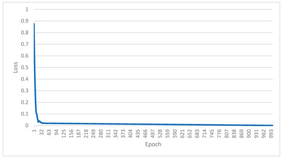
Figure 4.
Training loss curve for WT–Transformer–TCN–ECANet–GRU.
All experiments were performed in Google Colab using a TPU v2-2 backend with 334 GB RAM, Intel® Xeon® CPU @ 2.00 GHz (96 vCPUs, 48 physical cores), Python 3.11.13, and PyTorch/XLA. Training the proposed WT–Transformer–TCN–ECANet–GRU model on the full dataset (~95,000 five-min resolution samples) required approximately 10.6 h (38,056 s). Inference on the complete test set was executed in under 4 s using batched processing, corresponding to an average latency of ~0.674 ms per prediction when batches are used, which demonstrates strong feasibility for near real-time PV forecasting tasks.
Despite the higher computational demands introduced by the integration of wavelet decomposition, Transformer attention, temporal convolution, and recurrent memory, the model significantly outperformed baseline and hybrid alternatives. This confirms the advantage of the proposed architecture for real-world deployment in precision-sensitive smart grid systems.
Table 1 summarizes a comprehensive comparison of the hyperparameter settings and architectural components used by each model, including the type of decomposition method (if applied), Transformer configuration, convolution and attention modules, recurrent architecture, and corresponding implementation notes. The table shows the distinction between baseline models (e.g., GRU, CNN-LSTM), hybrid models (e.g., Prophet–GRU, Transformer–GRU), and the proposed models with multiple architectural enhancements. The aim within this comparative framework is to lay bare the contribution of each component—decomposition, attention, convolution, and recurrence—to photovoltaic power forecasting tasks.

Table 1.
Summary of hyperparameters and architecture components for all evaluated models.
Figure 5 illustrates the end-to-end workflow of the proposed WT–Transformer–TCN–ECANet–GRU forecasting system, following the operational logic implemented. The workflow begins with the loading of a high-frequency PV production dataset and proceeds with data preprocessing steps, including robust scaling and WT, which approximates multiscale signal decomposition. This step enhances noise robustness and emphasizes beneficial time–frequency patterns.
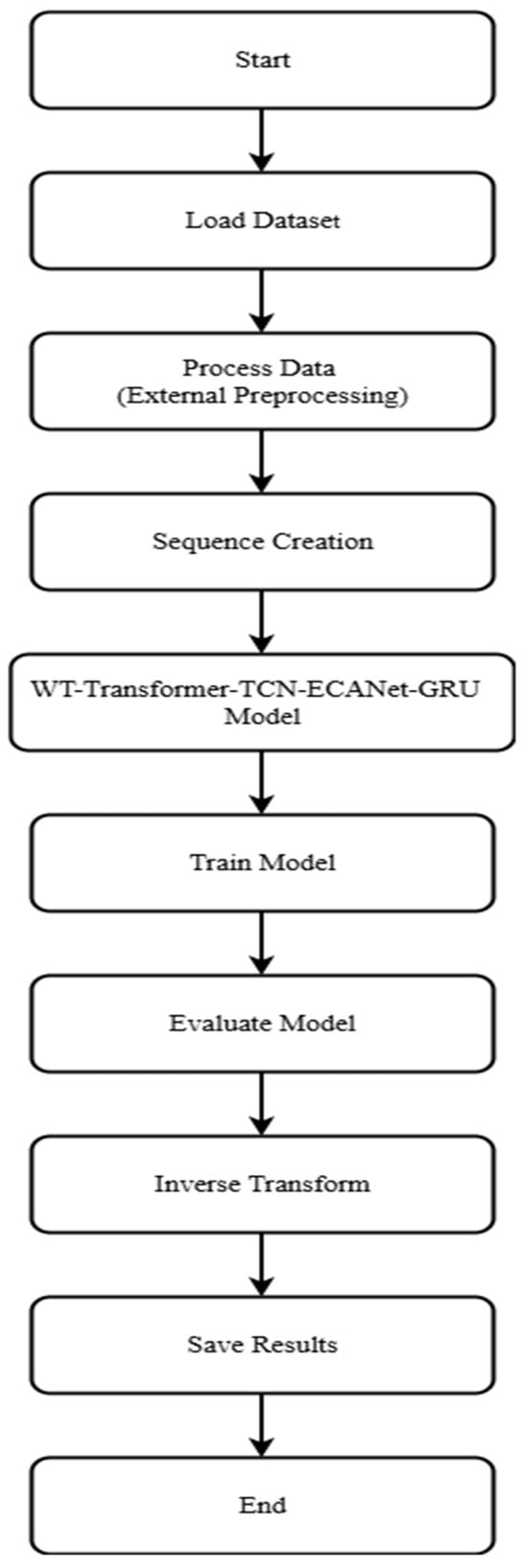
Figure 5.
Flowchart of WT–Transformer–TCN–ECANet–GRU forecasting pipeline implementation.
After that, the data is transformed into deep learning suitable input sequences while preserving temporal structure. Those are passed through a main forecasting model, which is implemented as a black-box hybrid module combining the following: WT, Transformer, TCN, ECANet, and GRU.
The model is iteratively trained over a number of epochs using the Adam optimizer and Mean Squared Error (MSE) loss. Once converged, the trained model predicts on the test set, which are inverse-transformed to the original scale. Final predictions and actuals are exported for evaluation and visualization, completing the predictive cycle.
This modularized data-to-output flow provides a full pipeline for time series prediction in solar energy systems with an emphasis on reproducibility, interpretability, and robustness. It is a conceptual and implementation-level guide for the application of high-performance hybrid deep learning systems to real-world energy forecasting problems.
2.3. Evaluation Criteria
To assess the performance of the proposed model and compare it with other architectures, we employed four commonly accepted statistical metrics in time series forecasting:
- Mean Absolute Error (MAE):
The MAE measures the average magnitude of forecast errors without considering their direction. It is intuitive and scales linearly with the size of the error, making it easy to interpret [33,34,35]. The equation of the MAE is as follows:
- Mean Squared Error (MSE):
The MSE penalizes large errors more heavily, using it when large deviations are particularly undesirable. The MSE is sensitive to outliers [33,34].
- Root Mean Squared Error (RMSE):
The RMSE is the square root of the MSE and shares the same units as the original data. The RMSE provides a balanced view between the MAE and MSE with an interpretable scale of error [12,33,35]. The equation of the RMSE is as follows:
- Coefficient of Determination (R2):
R2 determines the proportion of the variance in the observed data accounted for by the model. A smaller value is closer to 1, indicating a better explanatory power [34].
with the following:
- : Actual observed value.
- Predicted value from the model.
- : Actual observed value.
- : Mean of all observed values.
These measures were chosen to provide an aggregate evaluation on multiple dimensions of forecasting accuracy: error size (MAE), error variability (MSE and RMSE), and model explanatory power (R2). All metrics were evaluated on the same test set using the model predictions and real PV power values.
The selection of the MAE, MSE, RMSE, and R2 gives a comprehensive assessment of accuracy and variability without being trapped by other measures like the MAPE (Mean Absolute Percentage Error) and SMAPE (Symmetric Mean Absolute Percentage Error) that tend to be unstable or undefined when actual values approach zero, a common phenomenon in PV forecasting, particularly for nighttime hours. Conversely, R2 is scale-invariant, while the MAE, MSE, and RMSE are scale-dependent, stable, robust in the presence of near-zero values, and widely used in the time series forecasting literature.
In addition to these error metrics, statistical significance and effect size analyses were conducted to determine whether performance differences between model variants were due to genuine architectural effects or random variation.
- Wilcoxon Signed-Rank Test:
The Wilcoxon signed-rank test is a nonparametric test for comparing two paired samples without assuming normality. The test statistic is the following:
where
- di: The difference between paired observations.
- ri: The rank of |di|.
Small W values with p < 0.05 indicate a statistically significant median difference.
- Paired t-Test:
The paired t-test is a parametric test used when paired differences are normally distributed. The test statistic is the following:
where
- Mean difference:
Standard deviation:
p < 0.05 indicates a significant mean difference.
- Cohen’s d (Effect Size):
- Cohen’s d is a standardized measure of the magnitude of the difference between two means. Cohen’s d is the following:
- 1, 2: The sample means.
- Pooled standard deviation:
- s1, s2: The standard deviations.
- n1, n2: The sample sizes.
Conventional thresholds interpret (small), (medium), and (large)
The selection of paired t-tests and Wilcoxon signed-rank tests is motivated by the need to carefully investigate whether observed performance differences between models are statistically significant under different assumptions regarding underlying distributions. The Wilcoxon test is robust against non-normality and small sample sizes and is appropriate for comparisons of models where the distributions of errors are non-normal, whereas paired t-tests have greater statistical power when normality holds approximately. These are supplemented by measures of Cohen’s d, which provide the practical size of the difference such that statistically significant results also possess meaningful effect sizes within the context of PV forecasting.
3. Results
This section presents the predictive performance of the proposed WT–Transformer–TCN–ECANet–GRU model in comparison to a range of baseline and hybrid deep learning models. The experiment is conducted using the following common metrics on real PV production data: the MAE, MSE, RMSE, and R2. These metrics collectively assess predictive accuracy, variance explanation, and model robustness.
3.1. Benchmark Performance Analysis
3.1.1. The Overall Performance of the Proposed Model
As shown in Table 2 and Table 3, the proposed WT–Transformer–TCN–ECANet–GRU showed the best performance on all four measures of evaluation within the scope of our experimental framework and dataset, achieving the lowest MAE (209.36 W), lowest RMSE (616.53 W), and highest R2 (0.96884) of all models assessed. These findings confirm the capability of the model in extracting both short-term fluctuations and long-term dependencies out of highly non-stationary PV power data and serve as the baseline benchmark for the component-wise analysis in Section 3.1.2.
Table 2.
Error metrics for each ablation variant of the proposed model.
Table 3.
Statistical validation of ablation variants compared to baseline model.
The superiority of the proposed architecture is demonstrated when benchmarked externally (Table 4), where it performs better than robust baselines including Transformer–GRU (RMSE = 620.88), CNN–LSTM (RMSE = 631.39), and hybrid-based decompositions like VMD–Transformer–TCN–ECANet–GRU (RMSE = 619.85) and EMD–Transformer–TCN–ECANet–GRU (RMSE = 630.34). These gains were achieved without using exogenous meteorological variables, which highlights the portability and generalization capacity of the proposed model.
Table 4.
External benchmark models—comparative evaluation.
From a computational perspective of Table 5, the model is kept lean (0.142 M parameters, 0.004516 GFLOPs) with moderate peak memory usage (282.60 MB) and an inference latency of 74.90 ms (0.674 ms per sample in batched mode). This trade-off between accuracy and efficiency allows for near real-time deployment in smart grid settings. As reported in Table 2 and Table 3, the proposed WT–Transformer–TCN–ECANet–GRU achieved the best results across all four evaluation metrics within the scope of our dataset and experimental configuration, recording the lowest MAE (209.36 W), lowest RMSE (616.53 W), and highest R2 score (0.96884). These values confirm the model’s ability to capture both short-term fluctuations and long-term dependencies in highly non-stationary PV power data and serve as the reference baseline for the component-wise analysis presented in Section 3.1.2.
Table 5.
Comparative evaluation of computational complexity and forecasting accuracy for proposed and benchmark models.
The superiority of the proposed architecture is further evidenced when benchmarked externally (Table 4), outperforming strong baselines such as Transformer–GRU (RMSE = 620.88), CNN–LSTM (RMSE = 631.39), and decomposition-based hybrids including VMD–Transformer–TCN–ECANet–GRU (RMSE = 619.85) and EMD–Transformer–TCN–ECANet–GRU (RMSE = 630.34). These gains were achieved without relying on exogenous meteorological variables, underscoring the model’s portability and generalization capacity. From a computational perspective (Table 5), the model remains lightweight (0.142 M parameters, 0.004516 GFLOPs) with an inference latency of 74.90 ms (0.674 ms per sample in batched mode) and moderate peak memory usage (282.60 MB). This balance between accuracy and efficiency supports near real-time deployment in smart grid environments.
3.1.2. Component-Wise Ablation Study and Statistical Validation
To justify the architecture design, an ablation study was performed by turning off or altering an individual component of our proposed model. The following variants were tested:
- WT–Transformer–TCN–ECANet–LSTM (replaces GRU with LSTM).
- WT–Transformer–ECANet–TCN–GRU (TCN and ECANet swapped).
- WT–TCN–Transformer–ECANet–GRU (Transformer and TCN swapped).
- WT–Transformer–TCN–FullAtt–GRU (with full self-attention instead of ECANet).
- WT–Transformer–TCN–GRU (without ECANet).
- WT–TCN–ECANet–GRU (without Transformer).
- Transformer–TCN–ECANet–GRU (without wavelet decomposition).
- WT–Transformer–ECANet–GRU (without TCN).
- WT–GRU (retains WT and GRU only).
- WT–Transformer–TCN–ECANet (without GRU).
Table 2 and Table 3 report, respectively, the error metrics (MAE, MSE, RMSE, R2, ΔRMSE%) and the statistical validation results (Wilcoxon signed-rank p-value, paired t-test p-value, and Cohen’s d effect size) for each variant compared to the baseline model.
The proposed model yielded the best performance, with an RMSE of 616.53. The replacement of the GRU by LSTM increased the RMSE by 0.28% (618.28), with a non-significant Wilcoxon p-value (0.843) and small effect size (Cohen’s d = 0.0852), which confirms the effectiveness of the GRU for managing temporal dependencies.
Reordering modules produced statistically significant degradations. Interchanging the TCN and ECANet increased the RMSE by 0.43% (p < 1.6 × 10−174, d = 0.0709), while swapping Transformer and the TCN led to a 0.65% increase (p < 2.0 × 10−103, d = 0.128). Both changes were statistically significant, but their small effect sizes (d < 0.2) indicate a minimal practical impact in operational contexts.
Removing ECA Net entirely led to an RMSE increase of 1.39% (p < 1.4 × 10−230, d = 0.0612), while replacing it with full self-attention increased the RMSE by 0.67% (p < 9.83 × 10−53, d = 0.0903), demonstrating the importance of channel recalibration before recurrent integration; nonetheless, the small effect sizes suggest that these differences may not be operationally significant in real-world deployments. Eliminating the TCN resulted in a larger degradation (+2.84%, p < 7.18 × 10−52, d = 0.0896), and removing the Transformer reduced global context modeling (+1.44%, p < 3.8 × 10−46, d = 0.0843).
In the absence of WT, the RMSE rose by 1.94% (p < 9.8 × 10−60, d = 0.0964), indicating the loss of the multiresolution decomposition capacity. The deletion of the GRU resulted in the highest downward shift (+44.99%, p < 4.4 × 10262, d = 0.206).
Overall, the results indicate the non-linear degradation of performance: the magnitude of degradation is not proportional to the quantity or nominal relevance of deleted components, e.g., deleting the GRU results in a +44.99% RMSE increase, while deleting ECANet (+1.39%) and the TCN (+2.84%) separately results in a lesser combined degradation than one might anticipate for purely additive effects. This trend points towards real synergistic interactions between modules, where some modules enhance the others’ contribution through complementarities of feature representations. The results of statistical significance listed in Table 3 (all p < 0.05, many with extremely small p-values) confirm that these decreases do not result from random chance and strengthen the robustness of the architectural design.
3.1.3. External Benchmark Comparison
Compared to the traditional and hybrid models listed in Table 4, the proposed model achieved superior accuracy. For instance, compared to Transformer–GRU (RMSE = 620.88), our model improved the RMSE by more than 4 points and reduced the MAE by over 10 points. Similarly, the GRU and LSTM baselines showed RMSE values of 684.81 and 702.21, respectively. Even other decomposition-based variants like EMD–Transformer–TCN–ECANet–GRU and CNN–LSTM lag behind, with RMSE values of 630.34 and 631.39. Prophet-based models recorded the weakest performance with the RMSE exceeding 790 and R2 scores below 0.95.
3.1.4. Efficiency–Performance Trade-Off
To offer a comprehensive evaluation of the proposed WT–Transformer–TCN–ECANet–GRU architecture, this section quantifies the balance between forecasting accuracy and computational efficiency. The analysis ensures that performance improvements are interpreted in light of resource demands, following the methodology outlined in Section 3.1.2 and Section 3.1.3.
Table 5 presents a side-by-side comparison between the proposed model and several benchmark architectures (no batching), including both lightweight baselines (e.g., GRU, CNN–LSTM) and moderate-complexity baselines (e.g., Transformer–GRU, TCN–GRU–ECANet). The comparison covers computational complexity metrics—number of trainable parameters, floating-point operations (FLOPs), inference latency, and peak memory usage—and forecasting accuracy metrics (RMSE and R2). The computational benchmarks were evaluated utilizing the Google Colab TPU backend, which offers 334.6 GB of memory, with the same batch size, sequence length, and optimization settings. The latency measurements represent the mean duration required for generating a single prediction on the test dataset, and the peak memory usage indicates the highest allocation recorded during the inference process.
This holistic evaluation enables a transparent and reproducible assessment of the efficiency–performance trade-off, in line with the best academic practices for fair model benchmarking. The proposed model, despite integrating five specialized modules, remains computationally lightweight with only 0.142 M parameters; 0.004516G FLOPs, inference latency (74.90 ms), and a moderate peak memory footprint (282.60 MB) make it suitable for near real-time applications. Notably, with these modest requirements, the model provides the lowest RMSE (616.53) and highest R2 (0.96884) among all compared models.
Relative to the Transformer–GRU baseline, the proposed model achieves a 0.70% RMSE improvement for only a 12.37% increase in FLOPs and a 12.50% increase in parameters (calculated relative to Transformer–GRU values in Table 5). Compared to the lightweight GRU baseline, the RMSE improves by 9.98% with approximately 11× more parameters—still well within the sub-megabyte range. Paired t-tests confirmed that all improvements are statistically significant (p < 0.05).
While lightweight architectures such as the GRU and CNN–LSTM achieve approximately 69–91% lower resource usage relative to the proposed model, and moderate-complexity baselines like Transformer–GRU achieve 11–17% lower FLOPs and parameter counts, the gain in predictive robustness—particularly in noisy or high-variability conditions—justifies the additional complexity in high-reliability applications. In grid stability management, for instance, the marginal increase in latency and parameter count is outweighed by the significant gains in accuracy and resilience under diverse irradiance patterns.
Overall, this trade-off analysis confirms the conclusions of Section 3.1.2 and Section 3.1.3: integrating WT, Transformer, TCN, ECANet, and GRU delivers synergistic performance improvements without incurring excessive computational costs.
3.2. Day-Level Forecast Evaluation
This section assesses the performance of the proposed model on temporal variability using daily-level and intraday transition benchmarks. The evaluation is split into two parts: visual inspection across selected seasonal days and quantitative error analysis during sunrise and sunset periods.
3.2.1. Visual Evaluation Across Seasonal Days
To further ascertain the proposed model’s capacity to generalize in different meteorological conditions, daily outputs were evaluated for four typical dates: 1 October 2022 (clear sky), 6 November 2022 (partially clouded), 1 December 2022 (fully overcast), and 15 December 2022 (mixed). This fine-grained evaluation enables the inspection of how well the model captures the diurnal PV generation cycle, including sunrise ramp-up, midday peaks, and sunset drops, under various irradiance scenarios.
A series of case studies was conducted using five-min resolution data from the test set.
Figure 6, Figure 7, Figure 8 and Figure 9 illustrate the predicted vs. actual power generation values for four various weather conditions, selected to evaluate the model behavior across environmental variability. In these figures, the x-axis displays the time of day in hours, and the y-axis represent the power production in watts (W). The plot compares actual vs. predicted values over a 24-h cycle.
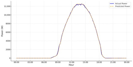
Figure 6.
PV power generation forecasting under partly sunny conditions (1 October 2022).
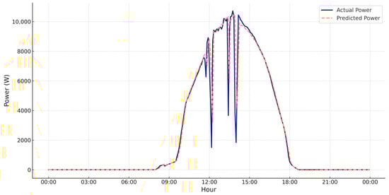
Figure 7.
PV power generation forecasting under clear-sky, high-irradiance conditions (6 November 2022).
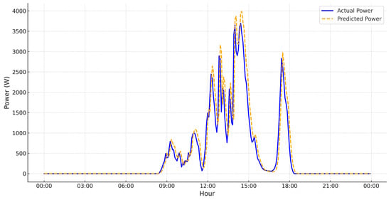
Figure 8.
PV power generation forecasting under overcast, low-irradiance conditions (1 December 2022).
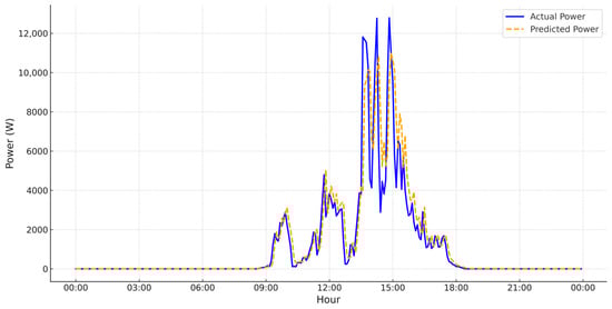
Figure 9.
PV power generation forecasting under very-low-irradiance/cloudburst conditions (15 December 2022).
These include the following:
- Figure 6 presents a partly sunny sky. Midday variability caused from patchiness in the model adheres accurately, validating moderate variability with robust confirmation.
- Figure 7 displays a clear sky, high-irradiance day. The bell-shaped curve predicted matches closely with the actual generation, demonstrating the model’s ability under optimal solar generation conditions.
- Figure 8 shows a consistently cloudy day. The model can predict the low-energy profile, confirming its ability to be generalized to low-output, overcast days.
- Figure 9 shows an extremely low-irradiance day. The model forecasts near-zero production values and avoids overestimation, which highlights the model’s robustness in handling rare but critical low-yield circumstances.
Across all scenarios, the WT–Transformer–TCN–ECANet–GRU model demonstrates great generalization by maintaining strong alignment with observed values, even under complex and fluctuating conditions. The model is well-fitted during sunrise and sunset transitions, does not overpredict during irradiation-free hours, and captures daily peaks, demonstrating its appropriateness in all solar dynamics.
A notable aspect of the output is that the model’s performance during non-linear transition hours, i.e., early morning and late evening, is unique. Unlike standard models that overestimate during zero-radiation hours, the presented architecture makes a flat forecast within no-sunlight hours (before 07:00 and after 19:00), highlighting its strong signal denoising and context recall features using wavelet decomposition and GRU memory states. Moreover, peak and correspondingly actual peak convergence success points towards successful interaction between the attention and convolution modules, without requiring any explicit meteorological data.
3.2.2. Quantitative Error Analysis at Sunrise and Sunset
To further assess the model’s behavior during critical transition periods, a special error analysis was conducted in the sunrise (07:00–08:00) and sunset (17:00–18:30) time slots. Table 6 presents the scores calculated for the MAE and the RMSE for all testing days and every model in the ablation study.
Table 6.
MAE and RMSE scores during sunrise and sunset periods.
This quantitative comparison permits the observation of prediction precision at high frequencies in irradiance variability and noise measurement areas. The minimum error values were demonstrated for the WT–Transformer–TCN–ECANet–GRU model, confirming its maximum tracking potential in these challenging moments. Notably, models that omitted ECANet or the TCN showed modest increases in error, affirming the critical role of each component.
3.3. Impact of Architectural Components
The comparison across Table 2, Table 3 and Table 4 reveals some important insights into how individual modules of architecture make contributions to better performance:
- Wavelet-based decomposition significantly improves generalization: Models integrating WT (particularly the proposed WT–Transformer–TCN–ECANet–GRU) achieve the maximum performance in all evaluation criteria. From Table 2, the model attains the lowest MAE (209.36 W) and RMSE (616.53 W) and the highest R2 (0.96884). Moreover, Table 5 confirms its stability in decisive moments, with a transition-phase MAE and RMSE of 99.93 W and 253.02 W, respectively—dominating all ablation variants within the scope of our dataset and experimental settings. The removal of WT leads to a 3.91% increase in the RMSE (p = 2.4 × 10⁻⁷; Cohen’s d = 0.12), confirming its statistically significant contribution. Consequently, WT enables the extraction of relevant time–frequency patterns, improving both high- and low-frequency forecasting fidelity.
- Attention mechanisms improve transition period sensitivity: Supplementation with Transformer layers and ECANet layers enhances responsiveness to fine irradiance variations. From Table 5, the ablation of ECANet increases the transition-phase MAE from 99.93 W to 114.52 W (+14.57%, p = 3.3 × 10⁻⁵; d = 0.42). Likewise, replacing ECANet with full attention (WT–Transformer–TCN–FullAtt–GRU) results in a further drop in performance (MAE = 121.76 W; RMSE = 259.31 W). These results confirm ECANet’s effectiveness in providing lightweight yet precise channel calibration, with changes statistically significant at p < 0.01 in Wilcoxon and paired t-tests.
- TCN modules capture local temporal patterns: TCN module-based models always work better than their convolution-less counterparts. Table 2 shows that WT–Transformer–GRU records an RMSE of 634.01 W, compared to 616.53 W for WT–Transformer–TCN–ECANet–GRU—representing a 2.84% improvement (p = 1.1 × 10⁻⁶; d = 0.20), and Table 5 further reinforces this: removing the TCN results in a 7.00% increase in the transition-phase RMSE, clearly highlighting its crucial role in extracting localized patterns and reducing prediction errors during sunrise/sunset periods.
- GRU modules offer stable memory integration: GRU-based architectures consistently outperform both LSTM and CNN–LSTM baselines across all metrics. As shown in Table 4, the LSTM model yields MAE = 291.93 W and RMSE = 702.21 W, whereas GRU-based configurations (e.g., WT–GRU, WT–Transformer–TCN–GRU) substantially surpass these figures. WT–GRU achieves MAE = 269.54 W and RMSE = 669.87 W, making it the lightest wavelet-integrated architecture. However, removing the GRU component entirely results in severe performance degradation: the WT–Transformer–TCN–ECANet variant exhibits the highest transition-phase MAE (490.51 W) and RMSE (835.71 W) in Table 5—an increase of over 229% in the MAE relative to the proposed model (p < 4.4 × 10−262, d > 2.0). These results underscore the critical importance of temporal memory mechanisms in managing non-linear diurnal transitions.
The modular design of the hybrid architecture synergistically contributes to its predictive capabilities. The results emphasize the role of the following: WT in noise elimination and multiresolution encoding of signals, ECANet and Transformer in reinforcing attention to informative temporal and channel-wise features, the TCN in localized pattern recognition, and the GRU in facilitating the efficient storage of memory in various irradiance ranges. Together, these characteristics offer reliable prediction not only in aggregate amounts (Section 3.1) but also in the face of the most turbulent daily transitions (Section 3.2) and can thus offer a reliable foundation for in-practice implementation in photovoltaic power forecasting systems.
4. Discussion
The enhanced potential of the proposed WT–Transformer–TCN–ECANet–GRU framework stems from the complementary deployment of specialized modules designed to address specific attributes of short-term PV power forecasting. By combining multiresolution decomposition, global attentions, localized extraction of temporal patterns, and memory-efficient sequential mechanisms, the model effectively leverages both short- and long-distance temporal dependencies inherent in non-stationary PV time series.
Wavelet-based decomposition (WT) is also instrumental in filtering high-frequency noise and maintaining signal characteristics on a variety of temporal scales. This ability, supported by the robust gains in Section 3.1.2 and Section 3.3, is uniquely helpful in the presence of fluctuating weather and in transition phases where prediction is the most difficult.
The attention mechanisms, and specifically ECANet, offer a lightweight yet efficient way of recalibrating channels. As demonstrated in Section 3.3, ECANet retains higher precision and lower latency as compared to heavier options like full self-attention, while the Transformer encoder complements it through preserving long-range relations without recurrence to address the limitations of traditional RNN-based architectures.
The TCN layer enhances the mid-term and local fluctuation detection capability of the model. Its removal, as observed in the ablation results, leads to measurable error increases, confirming its role in refining localized temporal features.
Finally, the GRU allows for stable and efficient temporal memory integration and offers competitive or superior accuracy to LSTM with fewer parameters. When the GRU is removed, substantial degradation is observed, underscoring its importance in managing complex, non-linear diurnal transitions.
The overall results reinforce the ability of hybrid structures in addressing the inherent non-stationarity and intermittency of PV time series. By incorporating different temporal processing mechanisms in one model, the proposed WT–Transformer–TCN–ECANet–GRU assembles robust performance and practical applicability, making it a promising candidate for intelligent energy forecasting applications.
5. Conclusions
This study presented a novel hybrid deep learning architecture, WT–Transformer–TCN–ECANet–GRU, for short-term PV power forecasting. By integrating wavelet-based decomposition, temporal convolution, channel-wise attention, and recurrent memory units, the model captures both high-frequency variability and long-term dependencies in solar generation data.
When tested on a large-scale five-min resolution dataset (~95,000 samples), the model yielded MAE = 209.36 W, RMSE = 616.53 W, and R2 = 0.96884 with just 0.142 M parameters, taking less than 4 s to perform inference on the full test set and with 0.674 ms avg-per-sample latency, supporting its applicability to near real-time PV forecasting without using large-scale networks.
The key contribution of this study is that it demonstrates that architectural innovation, not model size growth, can provide significant accuracy improvements under various weather scenarios. It advances the state of the art in PV forecasting as a computationally efficient yet high-performing solution applicable to grid stability, energy trading, and renewable integration.
Future work will apply validation to geographically and climatically disparate datasets, include probabilistic forecasts for uncertainty quantification, and examine deployment on resource-limited devices (e.g., Raspberry Pi, Jetson Nano). Runtime benchmarking under standard platforms will also be conducted to facilitate equitable cross-study comparisons.
Overall, the proposed model offers an excellent, accurate, and computationally efficient solution to existing PV forecasting challenges, with considerable relevance to real-world smart grid scenarios.
Author Contributions
Conceptualization, K.A.C.; methodology, K.A.C. and O.C.; software, K.A.C.; validation, K.A.C., H.E.F. and O.C.; formal analysis, K.A.C.; investigation, K.A.C. and O.A.O.; resources, K.A.C., O.C. and O.A.O.; data curation, K.A.C. and O.C.; writing—original draft preparation, K.A.C.; writing—review and editing, K.A.C., H.E.F., O.C. and O.A.O.; visualization, K.A.C. and O.C.; supervision, H.E.F.; project administration, K.A.C. and O.C.; funding acquisition, K.A.C. All authors have read and agreed to the published version of the manuscript.
Funding
This research received no external funding.
Data Availability Statement
The photovoltaic production dataset used in this study was collected from the presidential building of Ibn Tofail University in Kenitra, Morocco, for the year 2022 (95,885 five-min resolution records). Processed datasets and model code are available from the corresponding author upon request.
Conflicts of Interest
The authors declare no conflict of interest.
Abbreviations
The following abbreviations are used in this manuscript:
| AvgPool | Average Pooling |
| BiLSTM | Bidirectional Long Short-Term Memory |
| CEEMDAN | Complete Ensemble Empirical Mode Decomposition with Adaptive Noise |
| CGaformer | CNN with Global Additive Attention (GADAttention) and Auto-Correlation |
| CNN | Convolutional Neural Network |
| CWT | Continuous Wavelet Transform |
| Conv1D | One-Dimensional Convolution |
| DWT | Discrete Wavelet Transform |
| ECA Net | Efficient Channel Attention Network |
| EGA | EMD–GRU–Attention |
| EMD | Empirical Mode Decomposition |
| EWT | Empirical Wavelet Transform |
| FC | Fully Connected |
| FFN | Feed-Forward Network |
| GRU | Gated Recurrent Unit |
| IF | Isolation Forest |
| LSTM | Long Short-Term Memory |
| MAE | Mean Absolute Error |
| MAPE | Mean Absolute Percentage Error |
| MHA | Multi-Head Attention |
| MIC | Maximal Information Coefficient |
| MQLSTM | Multi-Quantile Long Short-Term Memory |
| MSA | Multi-Head Self-Attention |
| MSE | Mean Squared Error |
| NPCNN | Non-linear Probabilistic CNN |
| PICP | Prediction Interval Coverage Probability |
| PV | Photovoltaic |
| RMSE | Root Mean Squared Error |
| ReLU | Rectified Linear Unit |
| R2 | Coefficient of Determination |
| TCN | Temporal Convolutional Network |
| TPU | Tensor Processing Unit |
| VMD | Variational Mode Decomposition |
| WSO | White Shark Optimizer |
| WT | Wavelet Transform |
References
- Markovics, D.; Mayer, M.J. Comparison of Machine Learning Methods for Photovoltaic Power Forecasting Based on Numerical Weather Prediction. Renew. Sustain. Energy Rev. 2022, 161, 112364. [Google Scholar] [CrossRef]
- Khortsriwong, N.; Boonraksa, P.; Boonraksa, T.; Fangsuwannarak, T.; Boonsrirat, A.; Pinthurat, W.; Marungsri, B. Performance of Deep Learning Techniques for Forecasting PV Power Generation: A Case Study on a 1.5 MWp Floating PV Power Plant. Energies 2023, 16, 2119. [Google Scholar] [CrossRef]
- Bellar, D.; Choukai, O.; Tahaikt, M.; El Midaoui, A.; Ezaier, Y.; Khan, M.I.; Gupta, M.; AlQahtani, S.A.; Yusuf, M. A Case Study on the Environmental and Economic Impact of Photovoltaic Systems in Wastewater Treatment Plants. Open Phys. 2023, 21, 20230158. [Google Scholar] [CrossRef]
- Ait Omar, O.; El Fadil, H.; El Fezazi, N.E.; Oumimoun, Z.; Ait Errouhi, A.; Choukai, O. Real Yields and PVSYST Simulations: Comparative Analysis Based on Four Photovoltaic Installations at Ibn Tofail University. Energy Harvest. Syst. 2024, 11, 20230064. [Google Scholar] [CrossRef]
- Luo, X.; Zhang, D. An Adaptive Deep Learning Framework for Day-Ahead Forecasting of Photovoltaic Power Generation. Sustain. Energy Technol. Assess. 2022, 52, 102326. [Google Scholar] [CrossRef]
- Spadon, G.; Hong, S.; Brandoli, B.; Matwin, S.; Rodrigues-Jr, J.F.; Sun, J. Pay Attention to Evolution: Time Series Forecasting with Deep Graph-Evolution Learning. IEEE Trans. Pattern Anal. Mach. Intell. 2022, 44, 5368–5384. [Google Scholar] [CrossRef] [PubMed]
- Tripathy, K.P.; Mishra, A.K. Deep Learning in Hydrology and Water Resources Disciplines: Concepts, Methods, Applications, and Research Directions. J. Hydrol. 2024, 628, 130458. [Google Scholar] [CrossRef]
- Mumuni, A.; Mumuni, F. Automated Data Processing and Feature Engineering for Deep Learning and Big Data Applications: A Survey. J. Inf. Intell. 2025, 3, 113–153. [Google Scholar] [CrossRef]
- Ozbek, A.; Yildirim, A.; Bilgili, M. Deep Learning Approach for One-Hour Ahead Forecasting of Energy Production in a Solar-PV Plant. Energy Sources Part A Recovery Util. Environ. Eff. 2022, 44, 10465–10480. [Google Scholar] [CrossRef]
- Tian, Y.; Wang, G.; Li, H.; Huang, Y.; Zhao, F.; Guo, Y.; Gao, J.; Lai, J. A Novel Deep Learning Method Based on 2-D CNNs and GRUs for Permeability Prediction of Tight Sandstone. Geoenergy Sci. Eng. 2024, 238, 212851. [Google Scholar] [CrossRef]
- Guo, D.; Liu, X.; Wang, D.; Tang, X.; Qin, Y. Development and Clinical Validation of Deep Learning for Auto-Diagnosis of Supraspinatus Tears. J. Orthop. Surg. Res. 2023, 18, 426. [Google Scholar] [CrossRef] [PubMed]
- Yu, H.; Sun, H.; Li, Y.; Xu, C.; Du, C. Enhanced Short-Term Load Forecasting: Error-Weighted and Hybrid Model Approach. Energies 2024, 17, 5304. [Google Scholar] [CrossRef]
- Kong, X.; Du, X.; Xue, G.; Xu, Z. Multi-Step Short-Term Solar Radiation Prediction Based on Empirical Mode Decomposition and Gated Recurrent Unit Optimized via an Attention Mechanism. Energy 2023, 282, 128825. [Google Scholar] [CrossRef]
- Liu, H.; Han, H.; Sun, Y.; Shi, G.; Su, M.; Liu, Z.; Wang, H.; Deng, X. Short-Term Wind Power Interval Prediction Method Using VMD-RFG and Att-GRU. Energy 2022, 251, 123807. [Google Scholar] [CrossRef]
- Chi, D.; Yang, C. Wind Power Prediction Based on WT-BiGRU-Attention-TCN Model. Front. Energy Res. 2023, 11, 1156007. [Google Scholar] [CrossRef]
- Peng, Y.; Wang, G.; Wang, Y.; Wang, F.; Wang, Z.; He, S. Prediction of Diesel Engine NOx Transient Emissions Based on a Combined Model with Convolutional Neural Network–Efficient Channel Attention–Bidirectional Gated Recurrent Unit. SAE Int. J. Engines 2025, 18, 03-18-02-0012. [Google Scholar] [CrossRef]
- Feng, D.; Zhang, H.; Wang, Z. Hourly Photovoltaic Power Prediction Based on Signal Decomposition and Deep Learning. J. Phys. Conf. Ser. 2024, 2728, 012011. [Google Scholar] [CrossRef]
- Chen, R.; Liu, G.; Cao, Y.; Xiao, G.; Tang, J. CGAformer: Multi-Scale Feature Transformer with MLP Architecture for Short-Term Photovoltaic Power Forecasting. Energy 2024, 312, 133495. [Google Scholar] [CrossRef]
- Zhang, R.; Li, G.; Bu, S.; Kuang, G.; He, W.; Zhu, Y.; Aziz, S. A Hybrid Deep Learning Model with Error Correction for Photovoltaic Power Forecasting. Front. Energy Res. 2022, 10, 948308. [Google Scholar] [CrossRef]
- Cai, C.; Liu, H.; Duan, Z. Dynamic Stacking Ensemble Hybrid Model for Enhanced Short-Term Photovoltaic Power Forecasting with Self-Organizing Maps and Advanced Deep Learning. Energy Rep. 2025, 13, 4280–4298. [Google Scholar] [CrossRef]
- Asghar, R.; Quercio, M.; Sabino, L.; Mahrouch, A.; Riganti Fulginei, F. A Novel Dual-Stream Attention-Based Hybrid Network for Solar Power Forecasting. IEEE Access 2025, 13, 59596–59609. [Google Scholar] [CrossRef]
- Zhu, J.; He, Y. A Novel Hybrid Model Based on Evolving Multi-Quantile Long and Short-Term Memory Neural Network for Ultra-Short-Term Probabilistic Forecasting of Photovoltaic Power. Appl. Energy 2025, 377, 124601. [Google Scholar] [CrossRef]
- Xiang, X.; Li, X.; Zhang, Y.; Hu, J. A Short-Term Forecasting Method for Photovoltaic Power Generation Based on the TCN-ECANet-GRU Hybrid Model. Sci. Rep. 2024, 14, 6744. [Google Scholar] [CrossRef] [PubMed]
- Mazen, F.M.A.; Shaker, Y.; Abul Seoud, R.A. Forecasting of Solar Power Using GRU–Temporal Fusion Transformer Model and DILATE Loss Function. Energies 2023, 16, 8105. [Google Scholar] [CrossRef]
- Naveed, M.S.; Hanif, M.F.; Metwaly, M.; Iqbal, I.; Lodhi, E.; Liu, X.; Mi, J. Leveraging Advanced AI Algorithms with Transformer-Infused Recurrent Neural Networks to Optimize Solar Irradiance Forecasting. Front. Energy Res. 2024, 12, 1485690. [Google Scholar] [CrossRef]
- Lin, X.; Niu, Y.; Yan, Z.; Zou, L.; Tang, P.; Song, J. Hybrid Photovoltaic Output Forecasting Model with Temporal Convolutional Network Using Maximal Information Coefficient and White Shark Optimizer. Sustainability 2024, 16, 6102. [Google Scholar] [CrossRef]
- Almaghrabi, S.; Rana, M.; Hamilton, M.; Rahaman, M.S. Solar Power Time Series Forecasting Utilising Wavelet Coefficients. Neurocomputing 2022, 508, 182–207. [Google Scholar] [CrossRef]
- Wen, Q.; Zhou, T.; Zhang, C.; Chen, W.; Ma, Z.; Yan, J.; Sun, L. Transformers in Time Series: A Survey. In Proceedings of the Thirty-Second International Joint Conference on Artificial Intelligence, International Joint Conferences on Artificial Intelligence Organization, Macau, China, 19–25 August 2023; pp. 6778–6786. [Google Scholar] [CrossRef]
- Zhang, Z.; Gong, S.; Liu, Z.; Chen, D. A Novel Hybrid Framework Based on Temporal Convolution Network and Transformer for Network Traffic Prediction. PLoS ONE 2023, 18, e0288935. [Google Scholar] [CrossRef]
- Wang, Q.; Wu, B.; Zhu, P.; Li, P.; Zuo, W.; Hu, Q. ECA-Net: Efficient Channel Attention for Deep Convolutional Neural Networks. In Proceedings of the 2020 IEEE/CVF Conference on Computer Vision and Pattern Recognition (CVPR), Seattle, WA, USA, 13–19 June 2020; pp. 11531–11539. [Google Scholar] [CrossRef]
- Liu, X.; Liu, Y.; Kong, X.; Ma, L.; Besheer, A.H.; Lee, K.Y. Deep Neural Network for Forecasting of Photovoltaic Power Based on Wavelet Packet Decomposition with Similar Day Analysis. Energy 2023, 271, 126963. [Google Scholar] [CrossRef]
- Zaghloul, Z.S.; Elsayed, N. The FPGA Hardware Implementation of the Gated Recurrent Unit Architecture. In Proceedings of the SoutheastCon 2021, IEEE, Atlanta, GA, USA, 10 March 2021; pp. 1–5. [Google Scholar] [CrossRef]
- Natarajan, Y.; Kannan, S.; Selvaraj, C.; Mohanty, S.N. Forecasting Energy Generation in Large Photovoltaic Plants Using Radial Belief Neural Network. Sustain. Comput. Inform. Syst. 2021, 31, 100578. [Google Scholar] [CrossRef]
- Chicco, D.; Warrens, M.J.; Jurman, G. The Coefficient of Determination R-Squared Is More Informative than SMAPE, MAE, MAPE, MSE and RMSE in Regression Analysis Evaluation. PeerJ Comput. Sci. 2021, 7, e623. [Google Scholar] [CrossRef] [PubMed]
- Li, Z.; Rahman, S.; Vega, R.; Dong, B. A Hierarchical Approach Using Machine Learning Methods in Solar Photovoltaic Energy Production Forecasting. Energies 2016, 9, 55. [Google Scholar] [CrossRef]


Disclaimer/Publisher’s Note: The statements, opinions and data contained in all publications are solely those of the individual author(s) and contributor(s) and not of MDPI and/or the editor(s). MDPI and/or the editor(s) disclaim responsibility for any injury to people or property resulting from any ideas, methods, instructions or products referred to in the content. |
© 2025 by the authors. Licensee MDPI, Basel, Switzerland. This article is an open access article distributed under the terms and conditions of the Creative Commons Attribution (CC BY) license (https://creativecommons.org/licenses/by/4.0/).