Abstract
The neural architecture search technique is used to automate the engineering of neural network models. Several studies have applied this approach, mainly in the fields of image processing and natural language processing. Its application generally requires very long computing times before converging on the optimal architecture. This study proposes a hybrid approach that combines transfer learning and dynamic search space adaptation (TL-DSS) to reduce the architecture search time. To validate this approach, Long Short-Term Memory (LSTM) models were designed using different evolutionary algorithms, including artificial bee colony (ABC), genetic algorithm (GA), differential evolution (DE), and particle swarm optimization (PSO), which were developed to predict trends in global horizontal irradiation data. The performance measures of this approach include the performance of the proposed models, as evaluated via RMSE over a 24-h prediction window of the solar irradiance data trend on one hand, and CPU search time on the other. The results show that, in addition to reducing the search time by up to 89.09% depending on the search algorithm, the proposed approach enables the creation of models that are up to 99% more accurate than the non-enhanced approach. This study demonstrates that it is possible to reduce the search time of a neural architecture while ensuring that models achieve good performance.
1. Introduction
Designing and fine-tuning a suitable deep neural network (DNN) architecture has grown increasingly complex as applications demand ever more sophisticated models [1,2]. The common challenge lies in searching large, high-dimensional design spaces of layer configurations, hyperparameters, and connectivity patterns [3,4]. Conventional neural architecture search (NAS) methods address this problem by exhaustively or semi-exhaustively exploring candidate models [4]. However, doing so often proves computationally prohibitive [5]. Studies that adopt NAS frequently fail to address search-space redundancy, inadvertently prolonging search times for candidate architectures that offer only marginal gains [6,7]. Even more efficient search strategies frequently overlook how to prune unproductive subspaces or how to leverage knowledge gained from previously trained candidates [3].
To overcome these limitations, this work proposes a novel hybrid adaptive NAS approach which is specifically designed for global horizontal irradiance (GHI) trend forecasting. GHI is the total amount of solar radiation received per unit area by a horizontal surface on Earth, including both direct sunlight and diffuse sky radiation. GHI measures the solar power available on a flat surface, which is crucial for solar energy production. It influences the dimensioning of renewable energy systems and is used in solar panels and energy storage sizing [8]. Accurate prediction of GHI assists in the design and optimization of solar power systems, ensuring that they are efficient and cost-effective. Historical GHI data are available from the National Solar Radiation Database managed by the National Renewable Energy Laboratory and the Modern Era Retrospective Analysis for Research and Applications, Version 2 (MERRA-2), of NASA. GHI data can also be purchased from non-governmental sources such as the OpenWeather database [9].
The primary contributions of the proposed method encompass the following:
- Dynamic adaptation of the search spaces (DSS): In this study, we progressively refine the search space based on interim best models, preventing the exploration of redundant architectures and speeding up convergence;
- Reduction of exploration time via transfer learning (TL) and extrapolation techniques applied to the learning curve: The knowledge gained by high-performing architectures in initial phases is reused in subsequent generations, thus reducing time and resources, and training for unpromising candidate models is terminated early;
- The design of high-performance architectures through intelligent adaptive exploration.
Deep learning techniques are currently used in GHI prediction [10,11]. However, the effectiveness of these techniques depends on factors such as the neural network structure and hyperparameter tuning [12]. The selection and tuning of a suitable prediction model architecture is essential in deep learning applications [1]. Combining adaptive exploration, transfer learning, and extrapolation, the proposed NAS drastically reduces the architecture’s search time while maintaining high prediction accuracy. Our contributions unify multiple techniques into a single framework that accommodates complex, evolving models with lower computational overhead.
Experiments on historical datasets underscore the advantages of this hybrid approach. The method balances search efficiency by focusing on the most promising candidate architectures and predictive performance, as demonstrated by the RMSE score and significantly reduced NAS runtimes. This study shows that an intelligently curated, adaptive NAS can deliver high-performing and computationally feasible deep learning solutions.
2. Neural Architecture Search
NAS is a type of search technique for refining a predictive model such that it best represents the training data [2]. Similar to most search techniques, NAS has three components: (i) a search space containing feasible and unfeasible candidate architectures; (ii) a search strategy to explore the search space; and (iii) a performance estimation strategy, which is applied to the candidate architectures to provide feedback to the search strategy [3]. The following subsections provide an overview of these components in the context of GHI prediction.
2.1. Architecture Search Space
An architecture search space is used to determine which neural architectures are represented. A neural architecture can be defined as a three-tuple (a = (L, NL, Ha)), where L is the set of neural layers, NL is the number of neural layers constituting the architecture, and H is the set of hyperparameters belonging to neural architectures. Each architecture can have a different number of neurons, activation functions, dropout rates, learning rates, and batch sizes. Note that NL is not necessarily equal to the cardinality of the set L. From the above description, this study considers a search space S as a collection of neural architectures . Figure 1 provides a conceptual representation of a search space with NL = 6 neural layers, each having a different number of LSTM cells and hyperparameters. Part (S) of this figure is the initial state, where each layer can connect with others. It is a set of possible layers based on the space parameters. Part (a) shows a possible candidate architecture produced by a sample search strategy.
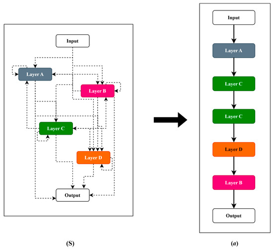
Figure 1.
(S) Search space and (a) a possible candidate architecture.
The definition of a candidate architecture depends on the values of its parameters, which in turn allow for definition of its characteristics.
2.2. Search Strategy
When building a neural architecture, a search strategy is used to explore the search space. It is responsible for ordering and connecting the layers L and selecting the architecture’s hyperparameter values. Given a collection of hyperparameters , we wish to find an architecture that minimizes an objective function f by selecting the appropriate hyperparameters (Equation (1)),
As in most search-oriented approaches, the function f guides the search strategy when exploring the search space. Most NAS strategies design a neural architecture by adding layers sequentially. An effective strategy would both avoid being trapped in local optima and have a fast execution time. Algorithms such as Bayesian optimization, evolutionary optimization, and reinforcement learning are currently used as search strategies [13]. In this context, the use of metaheuristic algorithms was proposed. This approach should enable the identification of an ideal compromise between exploring new architectures and leveraging existing ones. Thus, by defining as the hyperparameters identifying the best architecture being sought, the search strategy is defined by Equation (2):
The objective of the search strategy is to determine the vector of hyperparameters , which minimizes the objective function f (representing the root mean squared error in the context of this study).
2.3. Performance Estimation Strategy
Computing the objective function in (Equation (2)) represents a significant bottleneck regarding NAS execution time. The full training of neural architecture during the search process is computationally expensive and memory intensive [3,14]. Training with a reduced dataset can shorten execution time and often involves regularization techniques, such as dropouts and weight decay, to prevent overfitting. This ensures the model generalizes well to unseen data despite the dataset’s limited size. These methods, among others, enable deep learning models to achieve significant performance on small datasets [6,15]. Based on the above observation, this study proposes using transfer learning and learning curve extrapolation techniques to estimate the objective function value. Transfer learning is a machine learning concept in which a model previously developed for a specific task is reused as the basis for creating a new model for another task. Initially, this technique is used when the data labeled for the target task is scarce but abundant for another task. The application of transfer learning aims to utilize the knowledge of the source domain from the basic model to enhance learning in a second domain. This knowledge transfer is carried out by transferring the learned parameters, characteristics, and/or data representations from the original domain to the present research field [16]. Learning curve extrapolation is a technique that aims to predict the future performance of a model based on its past performance. It seeks to optimize the training process by estimating the performance of later stages, thereby reducing training wait time. This approach allows for learning about the continuation or cessation of the model’s training [17]. Adriaensen, Rakotoarison et al. [18] employed this approach to perform Bayesian inferences, predicting posterior distributions more accurately and efficiently than Monte Carlo methods. Under the same logic, Chandrashekaran and Lane [19] used learning curve extrapolation for hyperparameter optimization. In their study, each earlier trajectory is used to predict the next one, thereby eliminating poorly performing constructions and accelerating the search for hyperparameters. Let be the weights of the current best architecture found during a search process. We can estimate the weights of a new architecture by
where represents the total weight of the new layers added to . The weight refers to the parameters within the network (architecture) that are adjusted during the training process to minimize the error between the predicted output and the observed data. These weights are the scalar values multiplied by the input features or the output of neurons from the previous layer. By assuming x as the input vector, the output vector can be expressed as
with and representing the matrix of weights and biases for a given layer. Extrapolating the learning curve involves adding a stopping criterion during the training phase.
In Equation (5), P is the learning loss for candidate architecture at a given time t, and is the maximum time allowed. If the architecture does not improve, its training process is stopped because extrapolation will lead to an almost identical value at the end of its normal training cycle.
3. Proposed Approach of NAS Application
In the proposed approach, the methodology of designing neural architecture by applying NAS was adopted based on its demonstrated high capacity for hyperparameter adjustment [20], the model training process for weight adjustment [5], and model design [21]. Neural architecture design involves the application of various metaheuristics algorithms, including artificial bee colony (ABC), differential evolution (DE), genetic algorithm (GA), and particle swarm optimization (PSO), due to their unique approaches to solving optimization problems [22]. These methods have proven to be effective in managing high dimensionality in other fields. Zhou, Moayedi et al. [20] utilized ABC and PSO to develop Multi-Layer Perceptron architectures for predicting heating and cooling loads in residential buildings, achieving significantly greater accuracy than a natural design. Civicioglu and Besdok [23] evaluated ABC, PSO, Cuckoo-search (CK), and DE for their numerical problem-solving and found that DE provides more robust and accurate results than ABC, PSO, and CK. Sossa et al. [24] studied ABC, PSO, and DE to design neural network models for classification and pattern recall. Their work showed that these algorithms were more accurate in their architectures than non-heuristic approaches. These works have demonstrated their value in optimizing architectures to address extremely complex problems. This study combines metaheuristic algorithms with LSTM models, which, unlike RNN networks, can save information in their memories and, thus, be adapted for the prediction of time series [25]. Metaheuristic algorithms are employed in this research solely to construct the prediction model, i.e., to determine the optimal number of layers, the number of units in each layer, the optimal learning rate value, and the optimal dropout rate value. The model’s training is the sole responsibility of the backpropagation method [26]. This section starts by presenting the LSTM model architecture, followed by steps that describe the evolutionary algorithms studied in this research and their adoption in our approach. This section ends with the application case and the evaluation strategies utilized to validate the approach.
3.1. LSTM Model
LSTM (Long Short-Term Memory) models are a type of recurrent neural network (RNN). Originally, RNN models were derived from the Hopfield network for storing and associating models [27]. Recurrent neural networks are known for their ability to handle most long-distance prediction problems [28]. However, the disappearance of gradients in NNs is one of the main reasons that led to the development of the LSTM model. This model introduces internal trigger processes and memories for long-term information backup. The core component of LSTM is the memory cell, which maintains information over long periods. This helps the network to remember important information and forget irrelevant data. LSTMs use three types of gates to control the flow of information: (i) Input Gate determines which information from the current input should be added to the memory cell; (ii) Forget Gate decides what information should be discarded from the memory cell; and (iii) Output Gate controls what information from the memory cell should be output at each time step. The cell state acts as a conveyor belt, carrying relevant information through the sequence. The gates regulate the cell state, ensuring that important information is retained and irrelevant information is discarded. At each time step, LSTM processes the input data, updates the cell state, and produces an output. This allows the network to learn and remember patterns over long sequences. A detailed discussion on LSTM can be found in [29].
3.2. Metaheuristic Algorithms
This research focuses on four metaheuristic optimization algorithms: ABC, GA, DE, and PSO, which are described briefly in the following subsections. ABC performs a local search through cooperative ’bee’ behaviors, enabling a focused exploration around promising solutions. DE employs differential mutation, providing robustness and adaptability in high-dimensional search spaces. GA relies on genetic crossover operators to maintain an effective balance between diversity and intensification of the search. Finally, PSO uses particle dynamics to rapidly converge toward the most promising regions of the search space. The choice of these four metaheuristics covers a wide spectrum of exploration and exploitation strategies.
3.2.1. Artificial Bee Colony
The ABC swarm intelligence algorithm is a metaheuristic optimization algorithm inspired by bees’ foraging behavior [30,31]. Proposed in 2005 by Karaboga, the algorithm consists of three types of bees: employee, following, and scout bees [30]. Each group plays a crucial role in the search process. Employee bees are responsible for the overall exploration of the optimization problem, while follower bees are responsible for developing the best solutions. As for scout bees, their role is to put an end, when necessary, to the process of developing bad solutions. Applying the ABC algorithm to optimize the LSTM neural network architecture for predicting solar irradiance data begins with generating a population of individuals. Each individual or candidate solution is characterized by a set of parameters of dimension D, including the number of neurons on the input layer and the value of the learning rate, as well as several others. Each worker bee is then assigned a candidate solution. At each generation, the bees explore the search space around their current solution by modifying its parameters to discover new potential solutions , where is the new parameter value (for example, the learning rate); and represent the random coefficient used to update the value of the parameter and a randomly chosen value of the same parameter different from (the current value of the parameter), respectively. Next, based on the new candidate solutions provided by the worker bees, the observer or follower bees select the candidate architectures that will be used for the next generation, evaluating them according to the fitness function, in this case, the RMSE criterion. The scout bees’ role is to replace candidate architectures that fail to improve after a certain number of generations with new, randomly-generated candidate architectures.
3.2.2. Genetic Algorithm
Genetic algorithms (GAs) can be utilized to design an LSTM neural network architecture for predicting solar irradiance. The genetic process of biological organisms inspires these algorithms [32,33]. At each step, a genetic algorithm selects individuals from the current population to serve as parents and uses them to produce offspring for the next generation. Over successive generations, the population evolves toward a better solution. Each individual represents the candidate LSTM architecture to be evaluated in predicting the solar irradiance data. Each is composed of genes , and k is the generation number. The genes specify the values of hyperparameters, such as the number of neurons in a particular hidden layer, the type of activation function (ReLU, Sigmoid, or Tanh), the value of the learning rate, and many other factors that define an individual’s personality. A set of individuals is randomly generated at the start of the search. This population of LSTM networks is then improved by applying the genetic operators of crossover, mutation, and selection. Selection is based on the evaluation results of the previous generation’s objective function for candidate architectures. For this research, the objective criterion is represented by the RMSE function over a 24-h prediction window. After evaluating the population of a given generation, only the architectures that meet a specific passing condition, in this case, the individuals with a lower RMSE evaluation than the previous best in memory (for ), or a certain proportion of the best, will be selected. This process is the selection phase. At the end of the selection phase, the algorithm applies the crossover operation, which merges the previously selected individuals to form a new individual. Finally, the algorithm applies the mutation operation to the children resulting from the crossovers. This may modify the gene values, such as the number of neurons in the first hidden layer or the learning rate value. The new candidate architecture population is then formed for the next stage. This process is repeated until the stop condition is met.
3.2.3. Differential Evolution Algorithm
The differential evolution (DE) algorithm is a stochastic optimization method based on population evolution. Inspired by genetic algorithm operations, including selection, crossover, and mutation, this optimization method keeps the best particles unchanged from one iteration to the next. In contrast, other particles are replaced by new ones thanks to the above-mentioned operations [34]. This algorithm, therefore, implements four phases. An initialization phase, to create a random population of particles, and selection, crossover, and mutation phases, which give rise to the family of new particles to be evaluated. The algorithm begins by generating a family of solution vectors of dimensions D, representing the number of parameters to be optimized. In its general context, a DE algorithm is primarily inspired by the genetic algorithm and focuses particularly on its mutation and crossover processes. In the context of this research, at each generation, the DE algorithm creates a mutant vector for each of the individuals in the population. The mutant vector, therefore, represents a set of different values for the various parameters used to construct the candidate architecture for predicting solar irradiance data. This vector is created by adding the -weighted difference between two or more randomly selected individuals from the population to a final individual, also chosen randomly, thereby introducing diversity into the population. The process of forming the mutant vector from three individuals can be described as . By defining a combination rate, certain parameters are federated with the parameters of the current individual. This gives rise to a new set of individuals called the trial population. The DE algorithm then selects individuals by comparing the results of the objective function, i.e., the RMSE results of the current individual and its resulting trial. This selection defines the population to be considered for the next iteration. This process is repeated until the stopping condition is reached.
3.2.4. Particle Swarm Optimization
Particle swarm optimization (PSO) is a stochastic search algorithm. PSO is a multi-agent parallel search optimization technique first presented in 1995 by Kennedy and Eberhart [35]. This algorithm starts by randomly initializing the particles in the search space. Each potential solution is called a particle, and each particle has a random position and velocity at the start. As the algorithm unfolds, each particle adjusts its parameters by computing its new velocity (Equation (6)) and updating its position (Equation (7)).
As with the previous methods, finding the best LSTM architecture begins with randomly generating a set of individuals, known as particles. Each particle has a position at each time t representing the generation. The position defines the set of parameters used to build the architecture. In other words, the position includes the number of neurons on the layers and the values of the hyperparameters. The particle also has a velocity , which defines the rate of change and the direction as it explores the search space for each particle. Generation after generation, each particle stores the parameter values for its solution that obtains the best value of the objective function, the RMSE evaluation over a 24-h prediction window, represented by . At each generation, the algorithm updates the best position of the set of particles . Using the coefficients of inertia , confidence and , as well as random values and between 0 and 1, the algorithm defines the adjustments that need to be made to the various parameters, such as the number of neurons in the input layer, the number of neurons in the hidden layers, the learning rate, and many others, generation after generation. Ultimately, the final solution is considered the best among the different particle solutions. Similar to the methods mentioned above, the objective of the PSO application is to obtain the optimal architecture that strikes the best compromise between the complexity of the architecture and its performance.
3.2.5. Hyperparameter Encoding and Tuning
In the proposed method framework (ABC, DE, GA, and PSO), each individual in the population is represented by a “gene” vector encoding the neural network architecture hyperparameters.
- Neurons per input, hidden, and output layer (integer value): Governs model capacity and the bias-variance trade-off;
- Activation function (categorized as ReLU, Sigmoid, or Tanh): Affects nonlinearity, convergence speed, and gradient stability;
- Learning rate (continuous value): Controls weight update magnitude, balancing convergence speed and oscillations;
- Number of stacked LSTM units (integer): Adjusts temporal depth and sequential dependency modeling.
These hyperparameters capture the core dimensions of network complexity (capacity, depth, and nonlinearity) and search strategy (diversification and intensification). Using a uniform encoding across ABC, DE, GA, and PSO ensures fair comparison while leveraging their complementary mechanisms.
3.3. Solution Approach
For the proposed approach, the goal is to find a high-performance architecture that best represents the dataset and that can be achieved in a reasonable amount of time. To achieve these dual objectives, this study proposes an approach that dynamically adapts the search space and then applies transfer learning to reduce the time spent on model design. The methodology of this approach is illustrated in Figure 2. This study employs four metaheuristic algorithms—ABC, DE, GA, and PSO—to evaluate the proposed approach. The architectures are effectively the individuals these algorithms must optimize to obtain the most suitable architecture. In other words, the design process begins with generating a set of architectures. This set constitutes the first generation of the heuristic method.
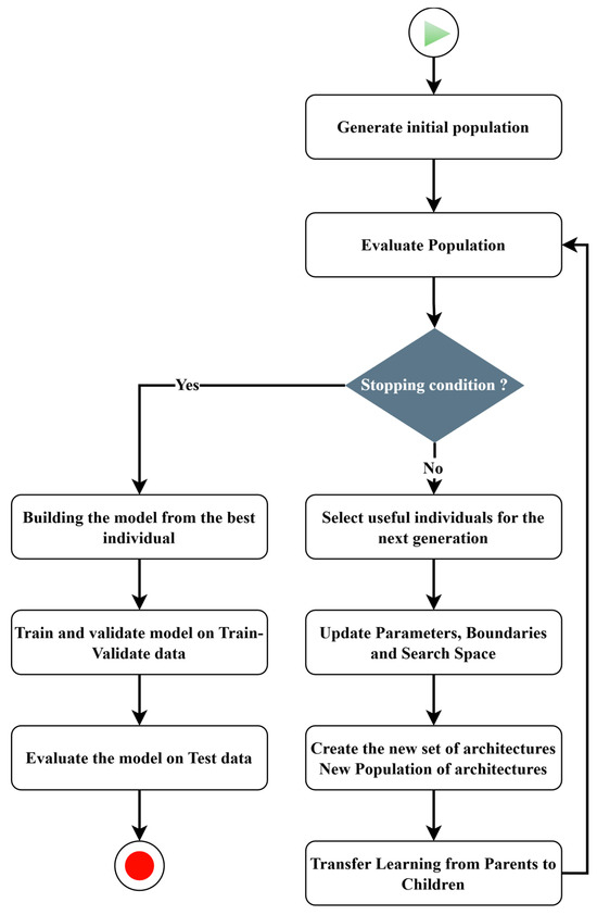
Figure 2.
Methodology: Presents the steps involved in the metaheuristic algorithms, from defining the initial population to determining the best architecture. These steps demonstrate the dynamic adaptation of the search space and the transfer of learning from parent architectures to new child architectures.
These candidate architectures are then evaluated by applying the performance estimation strategy of the neural architecture approach. Once this evaluation—which assesses the suitability function of the designated optimization method—is completed, the algorithm selects the architecture(s) with the best value of the suitability function according to its evolution process when the stop condition has not been reached. The search policy defines this stop condition. A new candidate architecture population is generated to produce new individuals from the previous candidate architectures. The evaluation processes, verification of the stop condition, and evolution of new populations continue until the stop condition is met. When the stop condition is reached, the best individual, in this case, the best architecture obtained, is used as the most representative model obtained by the metaheuristic optimization method. This process allows these metaheuristic algorithms to function as the main decision-makers of the architecture by reducing the researcher’s involvement in defining the final size (the number of layers and number of cells in each layer) of the prediction model to be designed, as well as the values of some hyperparameters (learning rate and dropout rates). All these processes are presented in Figure 2.
The pseudocode presented in Algorithm 1, along with Figure 2, describes the operating sequence of the proposed approach. This approach ensures an optimal compromise between search efficiency and predictive accuracy.
| Algorithm 1 Hybrid NAS with Transfer Learning and Dynamic Search Space |
|
Dynamic Search Space (DSS)
The definition of the search space is a crucial aspect in the design of neural architecture using the neural architecture search method [36]. This approach implements the definition of a dynamic search space (DSS) around the best solution from one population to another. In this search, the study defines S as the search space from which all possible candidate architectures are derived. Each of the candidate architectures is defined by a set of parameters . A fitness function then evaluates each architecture . The evaluation step then identifies the best architecture , defined by its parameters . Next, the proposed approach performs calibration operations around the best parameters to define the new search space. The search space update expression can be represented by , in which is the adjustment function. This approach enables continuous adjustment of the search space around the best architectures of previous populations as the search for the optimal architecture progresses, allowing for the definition of architectures with increasing numbers of layers while respecting the exploration stop condition. Thus, this process allows for level-by-level evolution, avoiding the evaluation of highly complex architectures from 0, which would likely not lead to the definition of the best overall architecture.
3.4. Application and Evaluation
To evaluate and validate this approach, it was applied in the context of the trend prediction of global horizontal irradiance data, and the CPU time required by each approach was measured. The training sessions were conducted on a computer equipped with a 2.8 GHz Intel processor and 16 GB of RAM. The computational performance was measured according to the execution time of the program, as determined via the process_time() method in the Python standard library, version 3.12.9. This method enabled the measurement of only the CPU time consumed by the current process, excluding periods of inactivity. The result returned is the time in seconds of the system mode. We eliminated the influence of any irrelevant activity by recording the CPU time just before and just after each algorithm run. The difference between these two times gives the CPU wait time for the program’s execution. This measure allows us to show the impact of the proposed solution on search time. However, to ensure that the time reduction this approach can enact does not have a strong negative effect on the models’ performance, performance measurements were recorded. The performance evaluation of the candidate architectures was carried out using the mean absolute error (MAE) and root mean squared error (RMSE). Equations (8) and (9) (below) express these performance measures.
where and are the values of the original (observed) and predicted data, respectively. n is the number of time series. Evaluation using MAE or RMSE means that the best models obtain lower values.
4. Results and Discussion
This research focused on three areas, one after the other. The first focus was on grid searching, with random searches for a high-performance architecture using the available data. Next, a neural architecture search was conducted, as defined by a non-enhanced approach using evolutionary algorithms. Finally, this study utilized the enhanced version of the neural architecture search, incorporating transfer learning (TL) and adapting dynamic search spaces (DSSs). The subsections below present the data acquisition, modeling, and parameters of the study, followed by the results of the three different approaches. This section concludes with a comparison of the other approaches.
4.1. Data Acquisition and Modeling
4.1.1. Data Acquisition
For this research, we collected historical global horizontal irradiance (GHI) data using École de technologie supérieure’s main campus (Latitude: 45.4948273 and Longitude: −73.5649115) as a reference point from the OpenWeather database [9]. The GHI data ranged from 2010 to 2020, segmented into distinct periods. The portion from 2010 to 2019 was used to train and validate the model, and the portion from 2019 to 2020 was used for the test phase. These time series data have several components: trend, seasonality, and residues.
4.1.2. Data Modeling
As an important first step, special attention was invested in data pre-processing. During this pre-processing phase, the data was cleaned, and the distribution of the missing data was carried out. The results of this first step showed that the missing data can qualify as completely random missing data (MCAR). These missing data were then imputed by the predictive mean matching (PMM) method [37]. Following the imputation of missing values and the analysis of outliers, a process of modeling the time series was undertaken [38]. This step enabled the decomposition of the data into a trend component, along with different seasonal components of 24 h and 24 h × 7 days, as well as a residual component. This method of decomposition, called multi-seasonal trend decomposition of time series (MSTL), is defined by Equation (10) and is inspired by the Loess STL decomposition method. The modeling method used in this study is the additive method.
In Equation (10), represents the data series at the moment t, and represent the trend and residuals of the series, respectively, and the seasonal components are represented by . Applying the MSTL multi-seasonal decomposition process to the time-series data allows the components , , and , which compose it, to be obtained. The trend allows for the representation of a long-term evolution of the series, the seasonality of the periodic phenomenon within the identified period (day, week), and finally, through the errors or residuals, the random component of the series. The second phase of data pre-processing involved data standardization, a step that brings the data back to a uniform value scale. Standardization is necessary before data analysis by the machine and deep learning models. Equation (11) presents the standardization operation using the min-max method.
Calculating ensures that each variable is projected in the same interval of values, preventing certain characteristics, with their higher amplitudes, from dominating the learning phase. More precisely, the minimum value is subtracted from each observation x. The result is then divided by the original range to obtain a normalized value between 0 and 1. Finally, multiplication by and the addition of min rescales the result to the target interval [min, max]. This homogeneous scaling operation facilitates model convergence and improves the robustness of estimates.
4.2. General Architecture Definition Parameters
This study considered a 12-h observation window (Loopback). The candidate architectures were trained to use a batch size of 32, the Adam optimizer, and the Sigmoid activation function, as outlined in Table 1 below. These specific parameter values were obtained following a sensitivity analysis involving 6-, 12-, and 24-h loopbacks, batch sizes of 16, 32, and 64, and two optimizers, Adam and Stochastic Gradient Descent (SGD). This analysis was conducted to design an architecture best-suited to a portion of the data by applying a genetic algorithm. This step was conducted in two stages, with the first focused on designing an architecture for some of the data. For this procedure, different LSTM layers and varied loop back values were defined (). This stage identified a set of best architectures, which were then evaluated in the second stage by varying the batch size (batchsize = {16, 32, 64}) and the optimizer between Adam and SGD. At the end of these experiments, the values that provided the best RMSE prediction for 6, 12, 24, and 48 h were retained for the rest of the research (Table 1).

Table 1.
Architecture training parameters.
Table 2 presents the different numbers of iterations and population sizes used to search for the optimal architecture that minimizes the RMSE (root mean squared error). The studied methods are all metaheuristic searches: artificial bee colony (ABC), differential evolution (DE), genetic algorithm (GA), and particle swarm optimization (PSO). During the metaheuristic optimization, we performed five full search cycles on the initial population and then reduced this to three cycles for each of the following populations. Each cycle corresponds to one complete application of the algorithm’s operators (mutation, crossover, and selection) rather than a training pass through the neural network. For all of the generations, the population size was kept at 10. We adopted these default values to avoid a lengthy exploration phase. However, for the grid search (GS), as the process is highly random, we defined a time limit as a constraint, rather than the constraints on iterations and population size.
Table 2.
Search parameters.
Table 3 summarizes the different design parameters optimized by the metaheuristic algorithms in this study. The learning rate, a crucial factor in weight adjustment during model training via gradient descent optimization, determines the scale of weight updates.
Table 3.
Search parameter boundaries.
Simultaneously, the dropout rate, specifying the proportion of randomly dropped neurons in hidden layers, mitigates overfitting by enhancing the generalization capacity of deep neural networks. Instead of using fixed values as the sensitivity step, the process used them as the hyperparameters that metaheuristics should optimize. Additionally, based on the results of the early phase of the sensitivity analysis, the number of LSTM units in each layer was added as a constraint, with a range of 64 to 128 for both the metaheuristic methods and the grid search approach. The proposed metaheuristic search does not restrict the architecture’s depth; instead, it evolves as a parameter within the metaheuristic method because the search space is updated step by step. However, for NAS without DSS and TL and using the grid search approach, the maximum depth of the architecture was set to 3, as defined in Table 3.
4.3. Detailed Results of Four Approaches
This subsection presents the results of the various experiments carried out, and we compare these approaches to demonstrate how the adopted approach can influence GHI prediction.
4.3.1. Grid Search Results
Grid architecture search (GS) yielded the best architectures in various simulations, with RMSE values of 0.0005 and 0.0015 for a 24-h prediction in two test cases, as specified by the parameters listed in Table 4. GS realized these results after a maximum search time of up to 100 CPU hours. The results of the GS evaluation over different forecast windows, ranging from 6 to 72 h, are summarized in Table 5.
Table 4.
Grid search best models details.
Table 5.
Grid search results for different forecasting windows.
Although this approach may require a long exploration time, it can provide better architectures, with an accuracy of 99% when the search intervals are well-defined. This implies that the researcher has a deep knowledge of the field. Moreover, since this search is entirely random, Table 5 shows that there is no guarantee of obtaining the same results from two different runs. The accuracy of two different executions may vary significantly due to the randomness of the approach.
4.3.2. Metaheuristics Results Without TL and DSS
The search time of the differential evolution (DE) method is considered the reference time for evaluating other methods. This approach’s estimated time (CPU time) is 875 h, 34 min, and 57.1 s. Table 6 presents the results of the architectural search for the four different methods adopted. It is clear that the genetic algorithm (GA) method is an optimal architecture, with a reduction from the DE’s time to 5.66%, i.e., 49 h, 35 min, and 40 s. However, the best RMSE rating on a 24-h prediction was achieved by the DE method, which was recorded at 0.0001. The third-ranked method was ABC-LSTM, with an evaluation of 0.0008 over 24 h of prediction and a time of 9.12% compared to that of the DE. PSO-LSTM scored 0.0010, with an estimated relative time of 23.35% of the DE method. Although GA has the shortest search time (5.66% of that of the DE method), it remains the method with the lowest estimated evaluation score of 0.0014. In conclusion, it is essential to note that, based on an assessment of the prediction, neural architecture search guided by the evolutionary algorithm (DE) yields better results; however, it requires a significantly longer search time. Therefore, the choice of algorithm guiding the search is a crucial aspect that warrants serious attention and consideration of the desired objectives.
Table 6.
Results without TL and DSS.
4.3.3. Metaheuristics Results with TL and DSS
The differential evolution (DE) method was also used as the reference for comparing exploration CPU times when combined with TL and DSS approaches.
DE is the method that required the longest search time, estimated at 166 h, 16 min, and 59 s. In this application, DE provides a better depth for a single architecture, with an estimated RMSE rating of 0.0005 for a 24-h prediction window, as shown in Table 7. Comparatively, the best evaluation results in terms of search time were obtained by PSO, GA, and ABC, in that order. PSO, with an estimated search time of 13.42% compared to that of DE, had an RMSE of 0.0001, while GA had an RMSE of 0.0003, with an estimated search time of 25.72%. ABC scored an RMSE of 0.0001, but with an estimated search time of 37.73% of the DE method’s time. Thus, the results indicate that applying the proposed approach allows for high-performance architectures to be obtained with significantly reduced search times.
Table 7.
Results with TL and DSS.
4.3.4. Comparison of the Results
We examined the different applications of grid search versus searches without it, and then with the application of transfer learning and a dynamic search space in the GHI trend prediction. The results show that GS scores well without TL and DSS. In a time-based comparison with DE, GS has the third-lowest search time, at 11.94% compared to DE, as shown in Table 8. The fourth position is occupied by the PSO method. While GS can provide a good architecture based on the proposed architecture’s performance, because it is a completely random process, it can often be less efficient. Moreover, compared to DE, when transfer learning and the dynamic adaptation of the search space are incorporated, the results show that the time set as a method stop condition is far higher than that of the ABC, GA, and PSO methods. In addition, the performances of the models obtained by using the ABC, DE, and PSO methods all improved with the inclusion of TL and DSS. Thus, the results indicate that the application of transfer learning, coupled with a dynamic adaptation of the search space, helps reduce search time and provides the architecture with improved performance.
Table 8.
Comparisons between GS and NAS approaches.
Table 9 compares approaches with and without transfer learning and dynamic search space adaptation for all four methods: ABC, DE, GA, and PSO. It is immediately obvious that without TL and DSS, all four methods require the longest computation time. The results show that even for the GA and ABC approaches, which generally require less time, the proposed approach reduces search time by 13.75 and 21.44%, respectively. This time reduction can be significant for the DE and PSO methods at 81.01 and 89.09%, respectively.
Table 9.
Direct comparison between our approaches and a non-enhanced approach.
In addition, the results show that, among all the methods, only the DE-LSTM method achieves an RMSE evaluation result without TL and DSS that is better than when applying TL and DSS, albeit with a very similar result, as shown in Table 9. Not only does this approach reduce the search time, but it also yields the best results in evaluations on the same dataset. Additionally, as presented in Table 6 and Table 7 above, the depth of architectures obtained without TL and DSS applications is greater than or equal to that of architectures with TL and DSS. However, the complexity of the architecture does not necessarily imply good adaptability to the data. Then, allowing methods to adapt and learn from their parents enables rapid convergence and fewer complex architectures without compromising accuracy.
Figure 3 and Figure 4 (above) show, on the x-axis, the number of candidate architectures evaluated by each algorithm according to the methodology adopted, and, on the y-axis, the root mean squared errors (RMSEs) obtained. These figures show that by applying the proposed TL and DSS approach, the worst RMSE rating obtained was only 0.175, whereas with the non-enhanced application of the NAS, the worst RMSE rating was 0.660. Moreover, although ABC achieves a higher number of evaluations of candidate architectures in the enhanced approach, the overall search time is shorter than with the non-enhanced approach. This shorter search time is achieved because the enhanced approach effectively controls the search space for designing candidate architectures. Finally, the results show that, although DE excels in accuracy with and without TL-DSS, its differential mutation strategy involves a high number of fitness assessments, resulting in a longer CPU time. Thus, the choice of methodology depends not only on the resources available (search time) but also on the accuracy of the model.
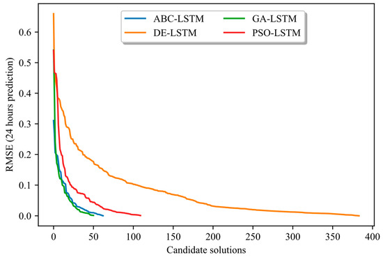
Figure 3.
NAS approach WITHOUT TL and DSS: Shows the number of candidate architectures evaluated per method and the order of magnitude of the RMSE errors obtained.
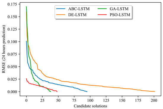
Figure 4.
NAS approach WITH TL and DSS: Shows the number of candidate architectures evaluated per method and the order of magnitude of the RMSE errors obtained.
Figure 5, Figure 6, Figure 7 and Figure 8 illustrate the normal evolution of the search space for the four candidate architectures.
Figure 5.
Proposed ABC candidate solutions’ evolution: Shows the number of candidate architectures and the order of magnitude of RMSE errors for the candidate architectures with and without TL-DSS.
Figure 6.
Proposed DE candidate solutions’ evolution: Shows the number of candidate architectures and the order of magnitude of RMSE errors for the candidate architectures with and without TL-DSS.
Figure 7.
Proposed GA candidate solutions’ evolution: Shows the number of candidate architectures and the order of magnitude of RMSE errors for the candidate architectures with and without TL-DSS.
Figure 8.
Proposed PSO candidate solutions’ evolution: Shows the number of candidate architectures and the order of magnitude of RMSE errors for the candidate architectures with and without TL-DSS.
These figures show that the proposed methodology achieves the following:
- Converges more quickly: Most of the error reduction occurs within the first 20–30 iterations for the proposed method. In contrast, the basic method often requires more than 50 iterations or even double that to achieve a comparable level of performance.
- Presents reduced variance: The red curves fluctuate much less and have a narrower envelope, reflecting more controlled and reliable progress. In contrast, the blue curves (approach without TL-DSS) frequently show declines and peaks of degradation, indicating ineffective evaluation.
- Achieves a more reliable final RMSE: In each of the figures, the end point of the red curve (approach with TL-DSS) is below that of the blue curve (approach without TL-DSS). This result shows that TL-DSS not only speeds up the search but also produces a more accurate architecture.
The results presented in these figures confirm that integrating transfer learning and dynamically adapting the search space leads to more efficient and stable NAS trajectories than the non-enhanced approach.
4.4. Comparison with Other Research
Table 10 presents a comparison of different neural architecture search (NAS) methods, highlighting the diversity of approaches and application areas covered by current research. Each method is distinguished by specific innovations tailored to various needs: ESC-NAS [12] targets the optimization of sound classification on edge devices by integrating hardware constraints. EGNAS [14] proposes an approach to accelerate architecture search for graph networks using evolutionary algorithms and weight sharing. Multi-objective approaches, such as that of [4], promote the discovery of efficient and diverse architectures through weight sharing and advanced evolutionary strategies. TrajectoryNAS [2], meanwhile, illustrates the importance of end-to-end optimization for real-time trajectory prediction, balancing accuracy and latency. Although these approaches have proven effective in their respective fields, none of them address the issue of search space, which can introduce dimensioning biases. Furthermore, search space optimization remains a common problem across all application domains. As a result, the method proposed in this study not only improves knowledge sharing but also dynamically optimizes the search space as the search evolves. It also avoids evaluation overtime, thanks to its learning curve extrapolation approach. This approach reduces search time by up to 89% while ensuring an accuracy of around 99%.
Table 10.
Comparison between the proposed approach and other related research.
5. Conclusions
The trend prediction of global horizontal irradiance data was used to validate the approach proposed in this study, involving the design of LSTM models by neural architecture search (NAS). This approach implements evolutionary methods to explore the search space using four different algorithms: artificial bee colony (ABC), genetic algorithm (GA), differential evolution (DE), and particle swarm optimization (PSO). The results show that using neural architecture search combined with the application of evolutionary algorithms yields excellent results, achieving an RMSE and MAE evaluation of over 99% within a 24-h prediction window. However, this approach remains very restrictive in terms of its time requirements. To address this issue, a hybrid learning approach was proposed, incorporating transfer learning and dynamic adaptation of the research space (TL-DSS). The results obtained when using this enhanced approach demonstrated that it is possible to significantly reduce research time while achieving equally efficient models. Incorporating TL-DSS can reduce the search time previously required for the ABC and GA algorithms by 21.44% and 13.75%, respectively. The reduction in search time reached 81.01% for DE and 89.09% for PSO.
In summary, this study makes three key contributions:
- Dynamic search space (DSS): Progressively refining the search space based on interim best models;
- Speed-up via transfer learning (TL) and learning curve extrapolation: Significantly reducing the NAS run time;
- High-performance architecture design through intelligent adaptive exploration: Balancing speed and predictive accuracy.
These contributions demonstrate the feasibility and effectiveness of the proposed approach for GHI forecasting while paving the way for future extensions.
Building on these contributions, several promising directions emerge:
- Extending dynamic NAS to Transformer-based time-series models, leveraging their self-attention mechanisms for long-range dependencies;
- Investigating conditional NAS for hybrid CNN–RNN or GNN architectures, allowing the search to jointly select model families and hyperparameters.
The obtained results suggest that exploring these avenues will further optimize the efficiency of searches and reveal powerful architectures in a wide range of application areas.
Author Contributions
Conceptualization, I.L., T.W. and L.-A.D.; methodology, I.L., T.W. and L.-A.D.; software, I.L.; validation, I.L., T.W. and L.-A.D.; formal analysis, I.L., T.W. and L.-A.D.; investigation, I.L.; resources, I.L., T.W. and L.-A.D.; data curation, I.L.; writing—original draft preparation, I.L.; writing—review and editing, T.W. and L.-A.D.; visualization, I.L.; supervision, T.W. and L.-A.D.; project administration, T.W. and L.-A.D.; funding acquisition, T.W. and L.-A.D. All authors have read and agreed to the published version of the manuscript.
Funding
This research was partially funded by the Natural Sciences and Engineering Research Council of Canada and by Innovee Québec.
Institutional Review Board Statement
Not applicable.
Informed Consent Statement
Not applicable.
Data Availability Statement
The original contributions presented in the study are included in the article; further inquiries can be directed to the corresponding author.
Conflicts of Interest
The authors declare no conflicts of interest.
Abbreviations
The following abbreviations are used in this manuscript:
| DNN | Deep Neural Network |
| NAS | Neural Architecture Search |
| GHI | Global Horizontal Irradiance |
| TL | Transfer Learning |
| DSS | Dynamic Search Spaces |
| RMSE | Root Mean Squared Error |
| MAE | Mean Absolute Error |
| MSE | Mean Squared Error |
| ABC | Artificial Bee Colony |
| GA | Genetic Algorithm |
| DE | Differential Evolution |
| PSO | Particle Swarm Optimization |
| RNN | Recurrent Neural Network |
| SOTA | State Of The Art |
| MSTL | Multi-seasonal Trend decomposition of Time-Series |
| MCAR | Missing Completely at Random |
| PMM | Predictive Mean Matching |
| SGD | Stochastic Gradient Descent |
| GS | Grid Search |
| MERRA-2 | Modern Era Retrospective Analysis for Research and Applications, Version 2 |
| CPU | Central Processing Unit |
References
- Shawki, N.; Nunez, R.R.; Obeid, I.; Picone, J. On Automating Hyperparameter Optimization for Deep Learning Applications. In Proceedings of the 2021 IEEE Signal Processing in Medicine and Biology Symposium (SPMB), Philadelphia, PA, USA, 4 December 2021; pp. 1–7. [Google Scholar] [CrossRef]
- Sharifi, A.A.; Zoljodi, A.; Daneshtalab, M. TrajectoryNAS: A Neural Architecture Search for Trajectory Prediction. Sensors 2024, 24, 5696. [Google Scholar] [CrossRef]
- Elsken, T.; Metzen, J.H.; Hutter, F. Neural architecture search: A survey. J. Mach. Learn. Res. 2019, 20, 1997–2017. [Google Scholar]
- Liang, J.; Zhu, K.; Li, Y.; Li, Y.; Gong, Y. Multi-Objective Evolutionary Neural Architecture Search with Weight-Sharing Supernet. Appl. Sci. 2024, 14, 6143. [Google Scholar] [CrossRef]
- Chitty-Venkata, K.T.; Emani, M.; Vishwanath, V.; Somani, A.K. Neural Architecture Search Benchmarks: Insights and Survey. IEEE Access 2023, 11, 25217–25236. [Google Scholar] [CrossRef]
- Xie, S.; Zheng, H.; Liu, C.; Lin, L. SNAS: Stochastic neural architecture search. arXiv 2018, arXiv:1812.09926v3. [Google Scholar]
- Niu, R.; Li, H.; Zhang, Y.; Kang, Y. Neural Architecture Search Based on Particle Swarm Optimization. In Proceedings of the 2019 3rd International Conference on Data Science and Business Analytics (ICDSBA), Istanbul, Turkey, 11–12 October 2019; pp. 319–324. [Google Scholar] [CrossRef]
- Mandal, A.K.; Sen, R.; Goswami, S.; Chakraborty, B. Comparative Study of Univariate and Multivariate Long Short-Term Memory for Very Short-Term Forecasting of Global Horizontal Irradiance. Symmetry 2021, 13, 1544. [Google Scholar] [CrossRef]
- OpenWeather. History Bulk weather data—OpenWeatherMap. Available online: https://openweathermap.org/history-bulk (accessed on 9 June 2023).
- Haider, S.A.; Sajid, M.; Sajid, H.; Uddin, E.; Ayaz, Y. Deep learning and statistical methods for short-and long-term solar irradiance forecasting for Islamabad. Renew. Energy 2022, 198, 51–60. [Google Scholar] [CrossRef]
- Chinnavornrungsee, P.; Kittisontirak, S.; Chollacoop, N.; Songtrai, S.; Sriprapha, K.; Uthong, P.; Yoshino, J.; Kobayashi, T. Solar irradiance prediction in the tropics using a weather forecasting model. Jpn. J. Appl. Phys. 2023, 62, SK1050. [Google Scholar] [CrossRef]
- Ranmal, D.; Ranasinghe, P.; Paranayapa, T.; Meedeniya, D.; Perera, C. ESC-NAS: Environment Sound Classification Using Hardware-Aware Neural Architecture Search for the Edge. Sensors 2024, 24, 3749. [Google Scholar] [CrossRef]
- Chitty-Venkata, K.T.; Emani, M.; Vishwanath, V.; Somani, A.K. Neural Architecture Search for Transformers: A Survey. IEEE Access 2022, 10, 108374–108412. [Google Scholar] [CrossRef]
- Jwa, Y.; Ahn, C.W.; Kim, M.J. EGNAS: Efficient Graph Neural Architecture Search Through Evolutionary Algorithm. Mathematics 2024, 12, 3828. [Google Scholar] [CrossRef]
- Baker, B.; Gupta, O.; Raskar, R.; Naik, N. Accelerating neural architecture search using performance prediction. arXiv 2017, arXiv:1705.10823. [Google Scholar]
- Best, N.; Ott, J.; Linstead, E.J. Exploring the efficacy of transfer learning in mining image-based software artifacts. J. Big Data 2020, 7, 59. [Google Scholar] [CrossRef]
- Viering, T.; Loog, M. The Shape of Learning Curves: A Review. IEEE Trans. Pattern Anal. Mach. Intell. 2023, 45, 7799–7819. [Google Scholar] [CrossRef]
- Adriaensen, S.; Rakotoarison, H.; Müller, S.; Hutter, F. Efficient bayesian learning curve extrapolation using prior-data fitted networks. Adv. Neural Inf. Process. Syst. 2024, 36, 19858–19886. [Google Scholar]
- Chandrashekaran, A.; Lane, I.R. Speeding up Hyper-parameter Optimization by Extrapolation of Learning Curves Using Previous Builds. In Proceedings of the Joint European Conference on Machine Learning and Knowledge Discovery in Databases, Skopje, Macedonia, 18–22 September 2017; Springer International Publishing: Cham, Switzerland, 2017; pp. 477–492. [Google Scholar] [CrossRef]
- Zhou, G.; Moayedi, H.; Bahiraei, M.; Lyu, Z. Employing artificial bee colony and particle swarm techniques for optimizing a neural network in prediction of heating and cooling loads of residential buildings. J. Clean. Prod. 2020, 254, 120082. [Google Scholar] [CrossRef]
- Telikani, A.; Tahmassebi, A.; Banzhaf, W.; Gandomi, A.H. Evolutionary machine learning: A survey. ACM Comput. Surv. (CSUR) 2021, 54, 1–35. [Google Scholar] [CrossRef]
- Karaboga, D.; Basturk, B. On the performance of artificial bee colony (ABC) algorithm. Appl. Soft Comput. 2008, 8, 687–697. [Google Scholar] [CrossRef]
- Civicioglu, P.; Besdok, E. A conceptual comparison of the Cuckoo-search, particle swarm optimization, differential evolution and artificial bee colony algorithms. Artif. Intell. Rev. 2013, 39, 315–346. [Google Scholar] [CrossRef]
- Sossa, H.; Garro, B.A.; Villegas, J.; Avilés, C.; Olague, G. Automatic Design of Artificial Neural Networks and Associative Memories for Pattern Classification and Pattern Restoration. In Proceedings of the 2012 Mexican Conference on Pattern Recognition, Huatulco, Mexico, 27–30 June 2012; Springer: Berlin/Heidelberg, Germany, 2012; pp. 23–34. [Google Scholar] [CrossRef]
- Li, G.; Yang, N. A Hybrid SARIMA-LSTM Model for Air Temperature Forecasting. Adv. Theory Simul. 2023, 6, 2200502. [Google Scholar] [CrossRef]
- de Campos Souza, P.V. Fuzzy neural networks and neuro-fuzzy networks: A review the main techniques and applications used in the literature. Appl. Soft Comput. 2020, 92, 106275. [Google Scholar] [CrossRef]
- Grollier, J.; Querlioz, D.; Camsari, K.Y.; Everschor-Sitte, K.; Fukami, S.; Stiles, M.D. Neuromorphic spintronics. Nat. Electron. 2020, 3, 360–370. [Google Scholar] [CrossRef] [PubMed]
- Gao, Y.; Yin, D.; Zhao, X.; Wang, Y.; Huang, Y. Prediction of Telecommunication Network Fraud Crime Based on Regression-LSTM Model. Wirel. Commun. Mob. Comput. 2022, 2022, 3151563. [Google Scholar] [CrossRef]
- Legrene, I.; Wong, T.; Dessaint, L.A. Horizontal Global Solar Irradiance Prediction Using Genetic Algorithm and LSTM Methods. In Proceedings of the 2024 IEEE 19th Conference on Industrial Electronics and Applications (ICIEA), Kristiansand, Norway, 5–8 August 2024; pp. 1–5. [Google Scholar] [CrossRef]
- Dokeroglu, T.; Sevinc, E.; Cosar, A. Artificial bee colony optimization for the quadratic assignment problem. Appl. Soft Comput. 2019, 76, 595–606. [Google Scholar] [CrossRef]
- Yang, Y.; Liu, D. A Hybrid Discrete Artificial Bee Colony Algorithm for Imaging Satellite Mission Planning. IEEE Access 2023, 11, 40006–40017. [Google Scholar] [CrossRef]
- Mehboob, U.; Qadir, J.; Ali, S.; Vasilakos, A. Genetic algorithms in wireless networking: Techniques, applications, and issues. Soft Comput. 2016, 20, 2467–2501. [Google Scholar] [CrossRef]
- Katoch, S.; Chauhan, S.S.; Kumar, V. A review on genetic algorithm: Past, present, and future. Multimed. Tools Appl. 2021, 80, 8091–8126. [Google Scholar] [CrossRef] [PubMed]
- Singsathid, P.; Puphasuk, P.; Wetweerapong, J. Adaptive differential evolution algorithm with a pheromone-based learning strategy for global continuous optimization. Found. Comput. Decis. Sci. 2023, 48, 243–266. [Google Scholar] [CrossRef]
- Kennedy, J.; Eberhart, R. Particle swarm optimization. In Proceedings of the ICNN’95—International Conference on Neural Networks, Perth, Australia, 27 November–1 December 1995; IEEE: Piscataway, NJ, USA, 1995; Volume 4, pp. 1942–1948. [Google Scholar] [CrossRef]
- Liu, Y.; Sun, Y.; Xue, B.; Zhang, M.; Yen, G.G.; Tan, K.C. A Survey on Evolutionary Neural Architecture Search. IEEE Trans. Neural Netw. Learn. Syst. 2023, 34, 550–570. [Google Scholar] [CrossRef]
- Akmam, E.F.; Siswantining, T.; Soemartojo, S.M.; Sarwinda, D. Multiple Imputation with Predictive Mean Matching Method for Numerical Missing Data. In Proceedings of the 2019 3rd International Conference on Informatics and Computational Sciences (ICICoS), Semarang, Indonesia, 29–30 October 2019; pp. 1–6. [Google Scholar] [CrossRef]
- Bandara, K.; Hyndman, R.J.; Bergmeir, C. MSTL: A Seasonal-Trend Decomposition Algorithm for Time Series with Multiple Seasonal Patterns. arXiv 2021, arXiv:2107.13462. [Google Scholar] [CrossRef]


Disclaimer/Publisher’s Note: The statements, opinions and data contained in all publications are solely those of the individual author(s) and contributor(s) and not of MDPI and/or the editor(s). MDPI and/or the editor(s) disclaim responsibility for any injury to people or property resulting from any ideas, methods, instructions or products referred to in the content. |
© 2025 by the authors. Licensee MDPI, Basel, Switzerland. This article is an open access article distributed under the terms and conditions of the Creative Commons Attribution (CC BY) license (https://creativecommons.org/licenses/by/4.0/).