
SegmentedCrossformer—A Novel and Enhanced Cross-Time and Cross-Dimensional Transformer for Multivariate Time Series Forecasting


Abstract
1. Introduction
2. Related Work
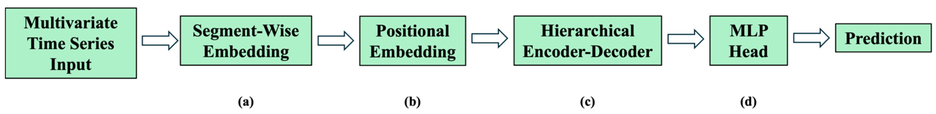
3. Methodology
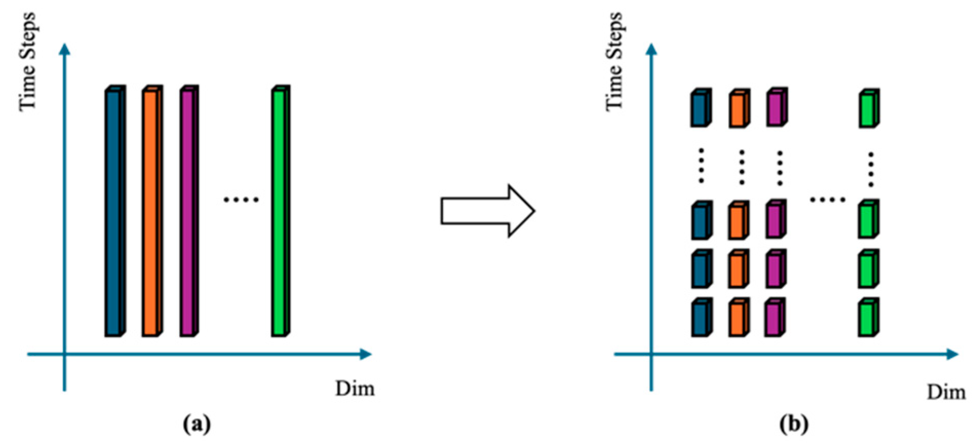
3.1. Time Series Segment-Wise Embedding
3.2. Two-Stage Attention
3.3. Hierarchical Encoder–Decoder
4. Experiments
4.1. Datasets
4.2. Setup
4.3. Model Results
4.4. Analysis and Discussion
5. Conclusions
Author Contributions
Funding
Data Availability Statement
Conflicts of Interest
Appendix A
Appendix A.1. Algorithms
| Algorithm A1 SegmentedCrossformer |
| 1: Inputs: 2: Multivariate Time Series with D dimensions in time step T, 3: Segment Length: 4: Embedded Dimension 5: Learnable Embedding Vector 6: Learnable Position Embedding Vector 7: Number of Heads in MSA: 8: Number of Current Encoder and Decoder Layers: 9: Learnable Position Embedding Vector: 10: Procedure SegmentedCrossformer(, , , , ): 11: # Initialization 12: Set Query Q, Key K and Value V 13: Set Learnable Embedding Vector 14: Set Learnable Position Embedding Vector 15: Set Learnable Position Embedding Vector: 16: # Implementation Starts from here 12: Set DimWiseEmbedding(, ) 13: Set 14: Set 15: # Hierarchical Encoder-Decoder to make the prediction 16: Set 17: return Y |
| Algorithm A2 Dimension-Wise Embedding |
| 1: Inputs: 2: Multivariate Time Series with D dimensions in time step T 3. Segment Length: 4: Procedure DimWiseEmbedding(): 6: Reshape into 7. Set x = 8. return x |
| Algorithm A3 Cross-Time Embedding |
| 1: Input: 2: Segmented Multivariate Time Series 3. Embedded Dimension 3: Learnable Embedding Vector 4: Learnable Position Embedding Vector 5: Procedure CrossTimeEmbedding(, , E, ): 6: Set Embedding Vector H = {} 7: Set = where and 7: for each segment in do: 8: Set 9: Set H = Concat(H, ) 10: end for 11: return H |
| Algorithm A4 Multihead Self-Attention (MSA) |
| 1: Require: Query: Q, Key: K, Value: V 2: Input: 3: Number of Heads in MSA: 4: Query: Q, Key: K, Value: V 5: Embedded Dimension: 6: Procedure MSA(Q, K, V, , ): 7: Set Y = {} 8: for do: 9: Set 10: Set , , and 11: Set 12: Set Y = Concat(Y, ) 13: end for 14: return Y |
| Algorithm A5 Two-Stage Attention |
| 1: Input: 2: 2D Embedding Vector 3: Require Query Q, Key K, Value V for Multi-head Self-Attention (MSA) 4: Number of Heads in MSA: 5: Embedded Dimension 6: 7: Procedure CrossTimeStage(H): 8: Set = {} 9: for do: 10: Set 11: Set 12: Set 13: Set 14: Set 15: end for 16: return 17: 18: Procedure CrossDimStage(H): 19. Set = {} 19: for do: 20: Set 21: Set learnable weight for linear projection and bias 22: Set 23: Set 24: Set 25: Set 26: Set 27: end for 28: return 29: 30: Procedure TwoStageAttn(H): 31: Set 32: Set 33: return Y |
| Algorithm A6 Hierarchical Encoder–Decoder (HED) |
| 1: Inputs: 2: Embedded Vector from TSA: H 3: Number of Current Encoder and Decoder Layers: 4: Learnable Position Embedding Vector: 5: Procedure Encoder(H, l): 6: if then: Set 9: else: Set 8: end if 9: return 10: 11: Procedure Decoder(H,l, ): 12: if = 1 then: Set 13: else: Set 14: end if 15: return 16: 17: Procedure HED(H,L, ,): 18: Set Y = 0 19: for do: 20: Set , 21: Set , 22: # update output for each encoder and decoder layer to be the input for next iteration 23: Set , 24: Set = {} 25: for do: 26: Set = , 27: Set 28: Set 29: end for 30: Set 31: Set 32: # make the prediction for by the sum for each layer 33: # Make inference for time series 34: Set 35: Set 36: end for 37: return Y |
Appendix A.2. Ablation Study

| Datasets | Metrics | Input Length | |||||
|---|---|---|---|---|---|---|---|
| 24 | 48 | 96 | 168 | 336 | 720 | ||
| ETTh1 | MSE | 0.551 | 0.593 | 0.538 | 0.464 | 0.531 | 0.913 |
| MAE | 0.510 | 0.534 | 0.529 | 0.496 | 0.529 | 0.695 | |
| ETTh2 | MSE | 0.118 | 0.111 | 0.526 | 1.057 | 0.913 | 1.957 |
| MAE | 0.220 | 0.217 | 0.445 | 0.705 | 0.684 | 1.137 | |
| WTH | MSE | 0.139 | 0.132 | 0.127 | 0.303 | 0.388 | 0.456 |
| MAE | 0.172 | 0.172 | 0.178 | 0.318 | 0.376 | 0.429 | |
| Datasets | ETTm1 | ETTm2 | Exchange-Rate | ||||
|---|---|---|---|---|---|---|---|
| Metrics | MSE | MAE | MSE | MAE | MSE | MAE | |
| Input length | 24 | 0.454 | 0.431 | 0.199 | 0.286 | 0.271 | 0.313 |
| 48 | 0.388 | 0.394 | 0.222 | 0.303 | 0.361 | 0.364 | |
| 96 | 0.342 | 0.377 | 0.338 | 0.382 | 2.335 | 1.161 | |
| 192 | 0.345 | 0.391 | 0.456 | 0.424 | 3.156 | 1.364 | |
| 288 | 0.365 | 0.396 | 0.690 | 0.544 | 2.464 | 1.281 | |
| 672 | 0.340 | 0.390 | 1.113 | 0.724 | 1.927 | 1.145 | |
| Datasets | ILI | ||
|---|---|---|---|
| Metrics | MSE | MAE | |
| Input length | 24 | 1.790 | 0.875 |
| 36 | 5.417 | 1.631 | |
| 48 | 2.679 | 1.020 | |
| 60 | 7.004 | 1.898 | |
Appendix A.3. Comprehensive Results
| Models | MTGNN | DLinear | LSTNet | LSTMa | STformer | SCF | |||||||
|---|---|---|---|---|---|---|---|---|---|---|---|---|---|
| Metric | MSE | MAE | MSE | MAE | MSE | MAE | MSE | MAE | MSE | MAE | MSE | MAE | |
| ETTh1 | 24 | 0.336 | 0.393 | 0.312 | 0.355 | 1.293 | 0.901 | 0.650 | 0.624 | 0.368 | 0.441 | 0.464 | 0.496 |
| 48 | 0.386 | 0.429 | 0.352 | 0.383 | 1.456 | 0.960 | 0.702 | 0.675 | 0.445 | 0.465 | 0.582 | 0.561 | |
| 168 | 0.466 | 0.474 | 0.416 | 0.430 | 1.997 | 1.214 | 1.212 | 0.867 | 0.652 | 0.608 | 0.972 | 0.725 | |
| 336 | 0.736 | 0.643 | 0.450 | 0.452 | 2.655 | 1.369 | 1.424 | 0.994 | 1.069 | 0.806 | 0.979 | 0.734 | |
| 720 | 0.916 | 0.750 | 0.486 | 0.501 | 2.143 | 1.380 | 1.960 | 1.322 | 1.071 | 0.817 | 0.985 | 0.758 | |
| ETTm1 | 24 | 0.260 | 0.324 | 0.217 | 0.289 | 1.968 | 1.170 | 0.621 | 0.629 | 0.278 | 0.348 | 0.342 | 0.377 |
| 48 | 0.386 | 0.408 | 0.278 | 0.330 | 1.999 | 1.215 | 1.392 | 0.939 | 0.445 | 0.458 | 0.465 | 0.453 | |
| 96 | 0.428 | 0.446 | 0.310 | 0.354 | 2.762 | 1.542 | 1.339 | 0.913 | 0.420 | 0.455 | 0.550 | 0.510 | |
| 288 | 0.469 | 0.488 | 0.369 | 0.386 | 1.257 | 2.076 | 1.740 | 1.124 | 0.733 | 0.597 | 0.745 | 0.613 | |
| 672 | 0.620 | 0.571 | 0.416 | 0.417 | 1.917 | 2.941 | 2.736 | 1.555 | 0.777 | 0.625 | 0.973 | 0.730 | |
| WTH | 24 | 0.307 | 0.356 | 0.357 | 0.391 | 0.615 | 0.545 | 0.546 | 0.570 | 0.307 | 0.359 | 0.127 | 0.178 |
| 48 | 0.388 | 0.422 | 0.425 | 0.444 | 0.660 | 0.589 | 0.829 | 0.677 | 0.381 | 0.416 | 0.203 | 0.256 | |
| 168 | 0.498 | 0.512 | 0.515 | 0.516 | 0.748 | 0.647 | 1.038 | 0.835 | 0.497 | 0.502 | 0.298 | 0.323 | |
| 336 | 0.506 | 0.523 | 0.536 | 0.537 | 0.782 | 0.683 | 1.657 | 1.059 | 0.566 | 0.564 | 0.388 | 0.376 | |
| 720 | 0.510 | 0.527 | 0.582 | 0.571 | 0.851 | 0.757 | 1.536 | 1.109 | 0.589 | 0.582 | 0.456 | 0.429 | |
| ILI | 24 | 4.265 | 1.387 | 2.940 | 1.205 | 4.975 | 1.660 | 4.220 | 1.335 | 3.150 | 1.232 | 4.287 | 1.406 |
| 36 | 4.777 | 1.496 | 2.826 | 1.184 | 5.322 | 1.659 | 4.771 | 1.427 | 3.512 | 1.243 | 5.417 | 1.631 | |
| 48 | 5.333 | 1.592 | 2.677 | 1.155 | 5.425 | 1.632 | 4.945 | 1.462 | 3.499 | 1.234 | 5.901 | 1.704 | |
| 60 | 5.070 | 1.552 | 3.011 | 1.245 | 5.477 | 1.675 | 5.176 | 1.504 | 3.715 | 1.316 | 7.005 | 1.898 | |
| Models | SCF | Informer | LogTrans | Reformer | LSTNet | LSTMa | |||||||
|---|---|---|---|---|---|---|---|---|---|---|---|---|---|
| Metric | MSE | MAE | MSE | MAE | MSE | MAE | MSE | MAE | MSE | MAE | MSE | MAE | |
| ETTh2 | 24 | 0.259 | 0.338 | 0.720 | 0.665 | 0.828 | 0.750 | 1.531 | 1.613 | 2.742 | 1.457 | 1.143 | 0.813 |
| 48 | 0.427 | 0.405 | 1.457 | 1.001 | 1.806 | 1.034 | 1.871 | 1.735 | 3.567 | 1.687 | 1.671 | 1.221 | |
| 168 | 1.057 | 1.057 | 3.489 | 1.515 | 4.070 | 1.681 | 4.660 | 1.846 | 3.242 | 2.513 | 4.117 | 1.674 | |
| 336 | 0.913 | 0.684 | 2.723 | 1.340 | 3.875 | 1.763 | 4.028 | 1.688 | 2.544 | 2.591 | 3.434 | 1.549 | |
| 720 | 1.957 | 1.957 | 3.467 | 1.473 | 3.913 | 1.552 | 2.015 | 4.625 | 4.625 | 3.709 | 3.963 | 1.788 | |
| ETTm2 | 24 | 0.199 | 0.286 | 0.173 | 0.301 | 0.211 | 0.332 | 0.333 | 0.429 | 1.101 | 0.831 | 0.580 | 0.572 |
| 48 | 0.223 | 0.303 | 0.303 | 0.409 | 0.427 | 0.487 | 0.558 | 0.571 | 2.619 | 1.393 | 0.747 | 0.630 | |
| 168 | 0.346 | 0.377 | 0.365 | 0.453 | 0.768 | 0.642 | 0.658 | 0.619 | 3.142 | 1.365 | 2.041 | 1.073 | |
| 336 | 0.712 | 0.550 | 1.056 | 0.804 | 1.090 | 0.806 | 2.441 | 1.190 | 2.856 | 1.329 | 0.969 | 0.742 | |
| 720 | 1.043 | 0.679 | 3.126 | 1.302 | 2.397 | 1.214 | 1.328 | 3.409 | 3.409 | 1.420 | 2.541 | 1.239 | |
| Models | Metric | Datasets | |||||||||||||||
|---|---|---|---|---|---|---|---|---|---|---|---|---|---|---|---|---|---|
| ETTh1 | ETTh2 | ETTm1 | ETTm2 | ||||||||||||||
| 96 | 192 | 336 | 720 | 96 | 192 | 336 | 720 | 96 | 192 | 336 | 720 | 96 | 192 | 336 | 720 | ||
| SCF | MSE | 0.771 | 1.136 | 0.979 | 0.985 | 0.905 | 1.007 | 0.913 | 1.957 | 0.538 | 0.701 | 0.756 | 1.033 | 0.316 | 0.456 | 0.712 | 1.043 |
| MAE | 0.658 | 0.794 | 0.734 | 0.758 | 0.650 | 0.698 | 0.684 | 1.137 | 0.496 | 0.597 | 0.622 | 0.752 | 0.458 | 0.424 | 0.550 | 0.679 | |
| FEDformer | MSE | 0.376 | 0.420 | 0.459 | 0.506 | 0.346 | 0.429 | 0.496 | 0.463 | 0.379 | 0.426 | 0.445 | 0.543 | 0.203 | 0.269 | 0.325 | 0.421 |
| MAE | 0.419 | 0.448 | 0.465 | 0.507 | 0.388 | 0.439 | 0.487 | 0.474 | 0.419 | 0.441 | 0.459 | 0.490 | 0.287 | 0.328 | 0.366 | 0.415 | |
| Autoformer | MSE | 0.449 | 0.500 | 0.521 | 0.514 | 0.358 | 0.456 | 0.482 | 0.515 | 0.505 | 0.553 | 0.621 | 0.671 | 0.255 | 0.281 | 0.339 | 0.422 |
| MAE | 0.459 | 0.482 | 0.496 | 0.512 | 0.397 | 0.452 | 0.486 | 0.511 | 0.475 | 0.496 | 0.537 | 0.561 | 0.339 | 0.340 | 0.372 | 0.419 | |
| Informer | MSE | 0.865 | 1.008 | 1.107 | 1.181 | 3.755 | 5.602 | 4.721 | 3.647 | 0.672 | 0.795 | 1.212 | 1.166 | 0.365 | 0.533 | 1.363 | 3.379 |
| MAE | 0.713 | 0.792 | 0.809 | 0.865 | 1.525 | 1.931 | 1.835 | 1.625 | 0.571 | 0.669 | 0.871 | 0.823 | 0.453 | 0.563 | 0.887 | 1.338 | |
| LogTrans | MSE | 0.878 | 1.037 | 1.238 | 1.135 | 2.116 | 4.315 | 1.124 | 3.118 | 0.600 | 0.837 | 1.124 | 1.153 | 0.768 | 0.989 | 1.334 | 3.048 |
| MAE | 0.740 | 0.824 | 0.932 | 0.852 | 1.197 | 1.635 | 1.604 | 1.540 | 0.546 | 0.700 | 0.832 | 0.820 | 0.642 | 0.757 | 0.872 | 1.328 | |
| Reformer | MSE | 0.837 | 0.923 | 1.097 | 1.257 | 2.626 | 11.12 | 9.323 | 3.874 | 0.538 | 0.658 | 0.898 | 1.102 | 0.658 | 1.078 | 1.549 | 2.631 |
| MAE | 0.728 | 0.766 | 0.832 | 0.889 | 1.317 | 2.979 | 2.769 | 1.697 | 0.528 | 0.592 | 0.721 | 0.841 | 0.619 | 0.827 | 0.972 | 1.242 | |
References
- Achiam, J.; Adler, S.; Agarwal, S.; Ahmad, L.; Akkaya, I.; Aleman, F.L.; Almeida, D.; Altenschmidt, J.; Altman, S.; Anadkat, S.; et al. GPT-4 Technical Report. arXiv 2023, arXiv:2303.08774. [Google Scholar] [CrossRef]
- Child, R.; Gray, S.; Radford, A.; Sutskever, I. Generating Long Sequences with Sparse Transformers. arXiv 2019, arXiv:1904.10509. [Google Scholar] [CrossRef]
- Devlin, J.; Chang, M.; Lee, K.; Toutanova, K. BERT: Pre-Training of Deep Bidirectional Transformers for Language Understanding. In Proceedings of the 2019 Conference of the North American Chapter of the Association for Computational Linguistics: Human Language Technologies, Minneapolis, MN, USA, 2–7 June 2019; pp. 4171–4186. [Google Scholar]
- Vaswani, A.; Shazeer, N.; Parmar, N.; Uszkoreit, J.; Jones, L.; Gomez, A.N.; Kaiser, Ł.; Polosukhin, I. Attention Is All You Need. In Proceedings of the 31st Conference on Neural Information Processing Systems (NIPS 2017), Long Beach, CA, USA, 4–9 December 2017; Luxburg, U., Guyon, I., Bengio, S., Wallach, H., Fergus, R., Eds.; pp. 6000–6010. [Google Scholar]
- Dosovitskiy, A.; Beyer, L.; Kolesnikov, A.; Weissenborn, D.; Zhai, X.; Unterthiner, T.; Dehghani, M.; Minderer, M.; Heigold, G.; Gelly, S.; et al. An Image Is Worth 16x16 Words: Transformers for Image Recognition at Scale. Presented at the International Conference on Learning Representations (ICLR 2021), Vienna, Austria, 3–7 May 2021. [Google Scholar]
- Wang, W.; Xie, E.; Li, X.; Fan, D.-P.; Song, K.; Liang, D.; Lu, T.; Luo, P.; Shao, L. Pyramid Vision Transformer: A Versatile Backbone for Dense Prediction Without Convolutions. In Proceedings of the 2021 IEEE/CVF International Conference on Computer Vision (ICCV), Montreal, QC, Canada, 10–17 October 2021; pp. 548–558. [Google Scholar] [CrossRef]
- Yan, W.; Sun, Y.; Yue, G.; Zhou, W.; Liu, H. FVIFormer: Flow-Guided Global-Local Aggregation Transformer Network for Video Inpainting. IEEE J. Emerg. Sel. Top. Circuits Syst. 2024, 14, 235–244. [Google Scholar] [CrossRef]
- Cao, Y.; Yu, H.; Wu, J. Training Vision Transformers with only 2040 Images. In Proceedings of the 17th European Conference (ECCV 2022), Tel Aviv, Israel, 23–27 October 2022; pp. 220–237. [Google Scholar] [CrossRef]
- Woo, G.; Liu, C.; Kumar, A.; Xiong, C.; Savarese, S.; Sahoo, D. Unified Training of Universal Time Series Forecasting Transformers. In Proceedings of the 41st International Conference on Machine Learning (ICML 2024), Vienna, Austria, 21–27 July 2024; pp. 53140–53164. [Google Scholar]
- Zhou, T.; Ma, Z.; Wen, Q.; Wang, X.; Sun, L.; Jin, R. FEDformer: Frequency Enhanced Decomposed Transformer for Long-term Series Forecasting. arXiv 2022, arXiv:2201.12740. [Google Scholar] [CrossRef]
- Wu, H.; Xu, J.; Wang, J.; Long, M. Autoformer: Decomposition Transformers with Auto-Correlation for Long-Term Series Forecasting. In Proceedings of the 35th International Conference on Neural Information Processing Systems (NIPS 21), Red Hook, NY, USA, 6–14 December 2021; pp. 22419–22430. [Google Scholar]
- Kitaev, N.; Kaiser, L.; Levskaya, A. Reformer: The Efficient Transformer. Presented at the International Conference on Learning Representations (ICLR 2020), Addis Ababa, Ethiopia, 26 April–1 May 2020. [Google Scholar]
- Zhou, H.; Zhang, S.; Peng, J.; Zhang, S.; Li, J.; Xiong, H.; Zhang, W. Informer: Beyond Efficient Transformer for Long Sequence Time-Series Forecasting. Presented at the AAAI Conference on Artificial Intelligence (AAAI-21), Virtually, 2–9 February 2021; Available online: https://cdn.aaai.org/ojs/17325/17325-13-20819-1-2-20210518.pdf (accessed on 20 March 2025).
- Nie, Y.; Nguyen, N.H.; Sinthong, P.; Kalagnanam, J. A Time Series Is Worth 64 Words: Long-Term Forecasting with Transformers. Presented at the 11th International Conference on Learning Representations (ICLR 2023), Kigali, Rwanda, 1–5 May 2023. [Google Scholar]
- Ghojogh, B.; Ghodsi, A. Recurrent Neural Networks and Long Short-Term Memory Networks: Tutorial and Survey. arXiv 2023, arXiv:2304.11461. [Google Scholar] [CrossRef]
- Graves, A. Generating Sequences with Recurrent Neural Networks. arXiv 2013, arXiv:1308.0850. [Google Scholar]
- Wu, Z.; Pan, S.; Long, G.; Jiang, J.; Chang, X.; Zhang, C. Connecting the Dots: Multivariate Time Series Forecasting with Graph Neural Networks. In Proceedings of the 26th ACM SIGKDD International Conference on Knowledge Discovery & Data Mining (KDD 20), Virtual Event, 6–10 July 2020; pp. 753–763. [Google Scholar] [CrossRef]
- Hochreiter, S.; Schmidhuber, J. Long Short-Term Memory. Neural Comput. 1997, 9, 1735–1780. [Google Scholar] [CrossRef] [PubMed]
- Zerveas, G.; Jayaraman, S.; Patel, D.; Bhamidipaty, A.; Eickhoff, C. A Transformer-based Framework for Multivariate Time Series Representation Learning. In Proceedings of the 27th ACM SIGKDD Conference on Knowledge Discovery and Data Mining (KDD 21), Singapore, 14–18 August 2021; pp. 2114–2124. [Google Scholar] [CrossRef]
- LeCun, Y.; Boser, B.; Denker, J.S.; Henderson, D.; Howard, R.E.; Hubbard, W.; Jackel, L.D. Backpropagation Applied to Handwritten Zip Code Recognition. Neural Comput. 1989, 1, 541–551. [Google Scholar] [CrossRef]
- Holt, C.C. Forecasting seasonals and trends by exponentially weighted moving averages. Int. J. Forecast. 2004, 20, 5–10. [Google Scholar] [CrossRef]
- Box, G.E.P.; Jenkins, G.M. Some Recent Advances in Forecasting and Control. J. R. Stat. Soc. Ser. C (Appl. Stat.) 1968, 17, 91–109. [Google Scholar] [CrossRef]
- Salinas, D.; Flunkert, V.; Gasthaus, J.; Januschowski, T. DeepAR: Probabilistic forecastingf with autoregressive recurrent networks. Int. J. Forecast. 2020, 36, 1181–1191. [Google Scholar] [CrossRef]
- Yan, C.; Wang, Y.; Zhang, Y.; Wang, Z.; Wang, P. Modeling Long- and Short-Term User Behaviors for Sequential Recommendation with Deep Neural Networks. In Proceedings of the 2021 International Joint Conference on Neural Networks (IJCNN), Shenzhen, China, 18–22 July 2021; pp. 1–8. [Google Scholar] [CrossRef]
- Chung, J.; Gulcehre, C.; Cho, K.; Bengio, Y. Empirical Evaluation of Gated Recurrent Neural Networks on Sequence Modeling. arXiv 2014, arXiv:1412.3555. [Google Scholar] [CrossRef]
- Cao, D.; Wang, Y.; Duan, J.; Zhang, C.; Zhu, X.; Huang, C.; Tong, Y.; Xu, B.; Bai, J.; Tong, J. Spectral temporal graph neural networks for multivariate time-series forecasting. In Proceedings of the 34th International Conference on Neural Information Processing Systems (NIPS 20), Vancouver, BC, Canada, 6–12 December 2020; pp. 17766–17778. [Google Scholar]
- Bai, L.; Yao, L.; Li, C.; Wang, X.; Wang, C. Adaptive graph convolutional recurrent network for traffic forecasting. In Proceedings of the 34th International Conference on Neural Information Processing Systems (NIPS 20), Vancouver, BC, Canada, 6–12 December 2020; pp. 17804–17815. [Google Scholar]
- Li, S.; Jin, X.; Xuan, Y.; Zhou, X.; Chen, W.; Wang, Y.X.; Yan, X. Enhancing the Locality and Breaking the Memory Bottleneck of Transformer on Time Series Forecasting. In Proceedings of the 33rd Conference on Neural Information Processing Systems, Vancouver, BC, Canada, 8–14 December 2019; pp. 5243–5253. [Google Scholar]
- Liu, S.; Yu, H.; Liao, C.; Li, J.; Lin, W.; Liu, A.X.; Dustdar, S. Pyraformer: Low-Complexity Pyramidal Attention for Long-Range Time Series Modeling. April 2022. Available online: https://openreview.net/pdf?id=0EXmFzUn5I (accessed on 17 March 2025).
- Zhang, Y.; Yan, J. Crossformer: Transformer Utilizing Cross-Dimension Dependency for Multivariate Time Series Forecasting. Presented at the 11th International Conference on Learning Representations (ICLR 2023), Kigali, Rwanda, 1–5 May 2023. [Google Scholar]
- Liu, X.; Wang, W. Deep Time Series Forecasting Models: A Comprehensive Survey. Mathematics 2024, 12, 1504. [Google Scholar] [CrossRef]
- Oreshkin, B.N.; Carpov, D.; Chapados, N.; Bengio, Y. N-BEATS: Neural basis expansion analysis for interpretable time series forecasting. Presented at the 8th International Conference on Learning Representations (ICLR 2020), Addis Ababa, Ethiopia, 26 April–1 May 2020. [Google Scholar]
- Liu, Z.; Lin, Y.; Cao, Y.; Hu, H.; Wei, Y.; Zhang, Z.; Lin, S.; Guo, B. Swin Transformer: Hierarchical Vision Transformer using Shifted Windows. In Proceedings of the 2021 IEEE/CVF International Conference on Computer Vision (ICCV), Montreal, QC, Canada, 17 October 2021; pp. 9992–10002. [Google Scholar] [CrossRef]

| Dataset Name | Dimensions | Total | Training | Validation | Testing |
|---|---|---|---|---|---|
| ETTh1 | 7 | 17,420 | 10,443 | 3481 | 3481 |
| ETTh2 | 7 | 17,420 | 10,405 | 3461 | 3461 |
| ETTm1 | 7 | 69,680 | 41,671 | 13,913 | 13,913 |
| ETTm2 | 7 | 69,680 | 41,797 | 13,931 | 13,931 |
| WTH | 21 | 52,696 | 31,570 | 10,517 | 10,517 |
| Exchange-Rate | 8 | 7588 | 4545 | 1516 | 1516 |
| ILI | 7 | 966 | 532 | 171 | 170 |
| Dataset | ETTh1 | ETTh2 | ETTm1 | ETTm2 | WTH | Exchange | ILI | |||||||
|---|---|---|---|---|---|---|---|---|---|---|---|---|---|---|
| Metrics | MSE | MAE | MSE | MAE | MSE | MAE | MSE | MAE | MSE | MAE | MSE | MAE | MSE | MAE |
| 4 | 0.273 | 0.342 | 0.111 | 0.217 | 0.117 | 0.209 | 0.109 | 0.202 | 0.050 | 0.084 | 0.228 | 0.290 | 1.641 | 0.777 |
| 6 | 0.343 | 0.379 | 0.126 | 0.236 | 0.158 | 0.244 | 0.140 | 0.240 | 0.060 | 0.096 | 0.324 | 0.342 | 2.305 | 0.917 |
| 12 | 0.453 | 0.447 | 0.179 | 0.282 | 0.258 | 0.324 | 0.152 | 0.245 | 0.078 | 0.127 | 0.577 | 0.492 | 2.835 | 1.097 |
| 24 | 0.464 | 0.496 | 0.259 | 0.338 | 0.342 | 0.377 | 0.211 | 0.289 | 0.132 | 0.172 | 1.413 | 0.791 | 4.287 | 1.406 |
| 48 | 0.583 | 0.561 | 0.427 | 0.405 | 0.454 | 0.472 | 0.222 | 0.303 | 0.222 | 0.264 | 2.048 | 1.109 | 5.901 | 1.704 |
| Models | Crossformer | FEDformer | Transformer | Informer | Autoformer | Pyraformer | SCF | LSTMa | MTGNN | ||||||||||
|---|---|---|---|---|---|---|---|---|---|---|---|---|---|---|---|---|---|---|---|
| Metric | MSE | MAE | MSE | MAE | MSE | MAE | MSE | MAE | MSE | MAE | MSE | MAE | MSE | MAE | MSE | MAE | MSE | MAE | |
| ETTh1 | 24 | 0.464 | 0.496 | 0.318 | 0.384 | 0.620 | 0.577 | 0.577 | 0.549 | 0.384 | 0.425 | 0.493 | 0.507 | 0.464 | 0.496 | 0.650 | 0.624 | 0.336 | 0.393 |
| 48 | 0.583 | 0.561 | 0.342 | 0.396 | 0.692 | 0.671 | 0.685 | 0.625 | 0.392 | 0.419 | 0.554 | 0.544 | 0.583 | 0.561 | 0.702 | 0.675 | 0.386 | 0.429 | |
| 168 | 0.410 | 0.441 | 0.412 | 0.449 | 0.947 | 0.797 | 0.931 | 0.752 | 0.490 | 0.481 | 0.781 | 0.675 | 0.464 | 0.496 | 1.212 | 0.867 | 0.466 | 0.474 | |
| 336 | 0.440 | 0.461 | 0.456 | 0.474 | 1.094 | 0.813 | 1.128 | 0.873 | 0.505 | 0.484 | 0.912 | 0.747 | 0.531 | 0.529 | 1.424 | 0.994 | 0.736 | 0.643 | |
| 720 | 0.519 | 0.524 | 0.521 | 0.515 | 1.241 | 0.917 | 1.215 | 0.896 | 0.498 | 0.500 | 0.993 | 0.792 | 0.913 | 0.695 | 1.960 | 1.322 | 0.916 | 0.750 | |
| ETTm1 | 24 | 0.211 | 0.293 | 0.290 | 0.364 | 0.306 | 0.371 | 0.323 | 0.369 | 0.383 | 0.403 | 0.310 | 0.371 | 0.342 | 0.380 | 0.621 | 0.629 | 0.260 | 0.324 |
| 48 | 0.300 | 0.352 | 0.342 | 0.396 | 0.465 | 0.470 | 0.494 | 0.503 | 0.454 | 0.453 | 0.465 | 0.464 | 0.457 | 0.444 | 1.392 | 0.939 | 0.386 | 0.408 | |
| 96 | 0.320 | 0.373 | 0.366 | 0.412 | 0.681 | 0.612 | 0.678 | 0.614 | 0.481 | 0.463 | 0.520 | 0.504 | 0.342 | 0.377 | 1.339 | 0.913 | 0.428 | 0.446 | |
| 288 | 0.404 | 0.427 | 0.398 | 0.433 | 1.162 | 0.879 | 1.056 | 0.786 | 0.634 | 0.528 | 0.729 | 0.657 | 0.365 | 0.396 | 1.740 | 1.124 | 0.469 | 0.488 | |
| 672 | 0.569 | 0.528 | 0.455 | 0.464 | 1.231 | 1.103 | 1.192 | 0.926 | 0.606 | 0.542 | 0.980 | 0.678 | 0.340 | 0.400 | 2.736 | 1.555 | 0.620 | 0.571 | |
| WTH | 24 | 0.294 | 0.343 | 0.357 | 0.412 | 0.349 | 0.397 | 0.335 | 0.381 | 0.363 | 0.396 | 0.301 | 0.359 | 0.132 | 0.172 | 0.546 | 0.570 | 0.307 | 0.356 |
| 48 | 0.370 | 0.411 | 0.428 | 0.458 | 0.386 | 0.433 | 0.395 | 0.459 | 0.456 | 0.462 | 0.376 | 0.421 | 0.203 | 0.256 | 0.829 | 0.677 | 0.388 | 0.422 | |
| 168 | 0.473 | 0.494 | 0.564 | 0.541 | 0.613 | 0.582 | 0.608 | 0.567 | 0.574 | 0.548 | 0.519 | 0.521 | 0.298 | 0.323 | 1.038 | 0.835 | 0.498 | 0.512 | |
| 336 | 0.495 | 0.515 | 0.533 | 0.536 | 0.707 | 0.634 | 0.702 | 0.620 | 0.600 | 0.571 | 0.539 | 0.543 | 0.388 | 0.376 | 1.657 | 1.059 | 0.506 | 0.523 | |
| 720 | 0.526 | 0.542 | 0.562 | 0.557 | 0.834 | 0.741 | 0.831 | 0.731 | 0.587 | 0.570 | 0.547 | 0.553 | 0.456 | 0.429 | 1.536 | 1.109 | 0.510 | 0.527 | |
| ILI | 24 | 3.041 | 1.186 | 2.687 | 1.147 | 3.954 | 1.323 | 4.588 | 1.462 | 3.101 | 1.238 | 3.970 | 1.338 | 4.287 | 1.406 | 4.220 | 1.335 | 4.265 | 1.387 |
| 36 | 3.406 | 1.232 | 2.887 | 1.160 | 4.167 | 1.360 | 4.845 | 1.496 | 3.397 | 1.270 | 4.377 | 1.410 | 5.417 | 1.631 | 4.771 | 1.427 | 4.777 | 1.496 | |
| 48 | 3.459 | 1.221 | 2.297 | 1.155 | 4.476 | 1.463 | 4.865 | 1.516 | 2.947 | 1.203 | 4.811 | 1.503 | 5.901 | 1.704 | 4.945 | 1.462 | 5.333 | 1.592 | |
| 60 | 3.640 | 1.305 | 2.809 | 1.163 | 5.219 | 1.553 | 5.212 | 1.576 | 3.019 | 1.202 | 5.204 | 1.588 | 7.005 | 1.898 | 5.176 | 1.504 | 5.070 | 1.552 | |
Disclaimer/Publisher’s Note: The statements, opinions and data contained in all publications are solely those of the individual author(s) and contributor(s) and not of MDPI and/or the editor(s). MDPI and/or the editor(s) disclaim responsibility for any injury to people or property resulting from any ideas, methods, instructions or products referred to in the content. |
© 2025 by the authors. Licensee MDPI, Basel, Switzerland. This article is an open access article distributed under the terms and conditions of the Creative Commons Attribution (CC BY) license (https://creativecommons.org/licenses/by/4.0/).
Share and Cite
Yang, Z.; Gonsalves, T. SegmentedCrossformer—A Novel and Enhanced Cross-Time and Cross-Dimensional Transformer for Multivariate Time Series Forecasting. Forecasting 2025, 7, 41. https://doi.org/10.3390/forecast7030041
Yang Z, Gonsalves T. SegmentedCrossformer—A Novel and Enhanced Cross-Time and Cross-Dimensional Transformer for Multivariate Time Series Forecasting. Forecasting. 2025; 7(3):41. https://doi.org/10.3390/forecast7030041
Chicago/Turabian StyleYang, Zijiang, and Tad Gonsalves. 2025. "SegmentedCrossformer—A Novel and Enhanced Cross-Time and Cross-Dimensional Transformer for Multivariate Time Series Forecasting" Forecasting 7, no. 3: 41. https://doi.org/10.3390/forecast7030041
APA StyleYang, Z., & Gonsalves, T. (2025). SegmentedCrossformer—A Novel and Enhanced Cross-Time and Cross-Dimensional Transformer for Multivariate Time Series Forecasting. Forecasting, 7(3), 41. https://doi.org/10.3390/forecast7030041