Abstract
This study addresses the challenge of predicting the airtightness of stratospheric airship envelopes, a critical factor influencing flight performance. Traditional ground-based airtightness tests often rely on limited resources and empirical formulas. To overcome these limitations, this paper explores the use of predictive models to integrate multi-source test data, enhancing the accuracy of airtightness assessments. A performance comparison of various prediction models was conducted using ground-based test data from a specific stratospheric airship. Among the models evaluated, the NeuralProphet model demonstrated superior accuracy in long-term airtightness predictions, effectively capturing time-series dependencies and spatial interactions with environmental conditions. This work introduces an innovative approach to modeling airtightness, providing both experimental and theoretical contributions to the field of stratospheric airship performance prediction.
1. Introduction
Stratospheric airships are near-space vehicles that rely on buoyancy from the lifting gas in the envelope to perform long-duration hovering missions [1]. The airship’s structural integrity is maintained by internal gas pressure, but factors like skin quality and welding processes inevitably cause leakage. When leakage becomes critical, the gas volume can no longer maintain the envelope’s inflation, leading to wrinkling and loss of aerodynamic shape, potentially disrupting buoyancy and causing altitude loss or a crash. Such issues can result in equipment damage, injuries, or fatalities. To ensure flight safety, airtightness tests should be conducted before missions to verify if the envelope’s airtight performance can support the required flight duration [2,3].
The key indicator of airtightness is the pressure differential between the internal gas and external atmospheric pressure. If this pressure falls below the minimum threshold for structural integrity during the test, it suggests that the envelope cannot meet the required flight duration. The differential pressure method is commonly used, observing the difference between internal pressure and atmospheric pressure in the testing environment [4].
Testing under actual stratospheric conditions is costly, so ground-based tests are preferred. However, due to the large volume of airship envelopes and long flight durations, these tests require significant resources. Predictive performance methods, using short-term data, can help reduce testing costs. These methods can be model-driven or data-driven. Model-driven approaches are resource-intensive and complex, especially when dealing with nonlinearities. In contrast, data-driven methods, especially those using machine learning, bypass the limitations of physical modeling and can identify patterns without explicit assumptions. These methods handle complex, nonlinear relationships, scale well with large datasets, and optimize model performance through automatic feature selection.
Data-driven prediction methods bypass the inherent limitations of physical modeling, with machine learning playing a central role in these approaches [5]. This paper focuses on the selection and comparison between traditional machine learning models and deep learning models. Unlike traditional physical modeling, which relies on assumptions and prior knowledge, both traditional machine learning and deep learning models can automatically learn from large datasets and uncover underlying patterns without explicit physical assumptions. These methods effectively handle complex nonlinear relationships, scale to large datasets, and optimize model performance through automatic feature selection [6,7]. The main contributions of this paper are as follows:
- (1)
- Correlation Analysis of Features: This study examines the linear correlations between various features in the dataset;
- (2)
- Model Selection and Comparison: Common machine learning models are selected and compared based on their predictive performance on the sample dataset;
- (3)
- Result Analysis: The long-term prediction results of each model are analyzed for validity, demonstrating the superiority of the NeuralProphet model in predicting the airtightness of stratospheric airships.
2. Data Preprocessing and Sample Partitioning
2.1. Data Preprocessing
This study’s dataset is sourced from the envelope airtightness ground testing data of a specific airship, collected by the affiliated organization from 13:25:00 on 25 April 2023, to 13:50:00 on 4 May 2023. Figure 1 displays the variation curves of the following parameters from the original data: indoor atmospheric pressure, the difference between the internal gas pressure of the envelope and the external atmospheric pressure, the external gas temperature, and the internal gas temperature of the envelope.
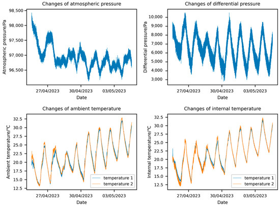
Figure 1.
Original data.
The difference between the internal gas pressure of the envelope and the external atmospheric pressure is the key indicator for determining the airtightness of the envelope, which is the prediction target of this study. Before integrating the sample set, the correlations between the features must be analyzed. For the five physical quantities—calculated internal atmospheric pressure, measured pressure difference, external gas temperature, and internal gas temperature—the Pearson correlation coefficient is used to assess the linear relationship between each pair of variables. The formula for calculating the Pearson correlation coefficient is given in Equation (1).
Given a set of sample points with data points, the Pearson correlation coefficient ranges from −1 to 1, with the following interpretation: indicates no linear correlation; indicates a negative correlation; indicates a positive correlation. A linear correlation is generally considered significant when [8]. The linear correlation plot for the features, shown in Figure 1, is presented in Figure 2, with the Pearson correlation coefficients indicated.
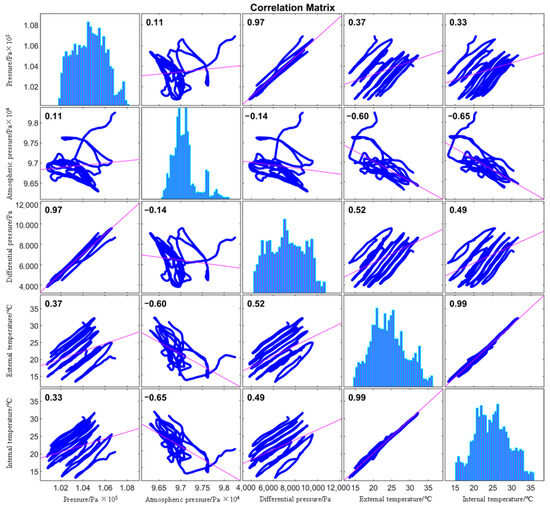
Figure 2.
Correlation graphs for actual measured physical quantities.
The histograms on the plot’s diagonal display the distribution of each feature. The gas pressure difference inside and outside the envelope is relatively uniform, while atmospheric pressure, environmental temperature, and internal gas temperature are more concentrated. The pink line in the figure represents the linear regression fit, whose slope corresponds to the Pearson correlation coefficient, indicating the proportional relationship between the variables.
The Pearson correlation coefficient between atmospheric pressure and pressure difference indicates the weakest correlation among the features. Atmospheric pressure shows a negative linear correlation with both environmental and internal temperatures, while the pressure difference has a positive linear correlation with both temperatures. Notably, the Pearson coefficient between environmental and internal gas temperatures is , indicating a strong positive correlation. This indicates that the covariance matrix of these two features approaches singularity, potentially leading to numerical instability during matrix inversion and erratic parameter updates in model training. Their high entropy overlap implies redundant information, where retaining both features increases computational burden without enhancing predictive capability. Feature removal thus simplifies the model architecture and improves convergence while preserving accuracy. Although dimensionality reduction can typically be achieved through PCA (Principal Component Analysis) without feature elimination while avoiding redundancy, the technical benefits of this processing may prove inferior to its operational costs when , rendering direct feature removal a more computationally efficient alternative.
As a result, we excluded internal gas temperature. The input and output features used in the study are shown in Table 1.

Table 1.
Input–output feature configuration.
Let the current time step corresponding to the predicted pressure difference be . The data observed between the time steps and is considered as the historical data, which serves as the input feature for the model. The value of can be modified according to the model’s requirements.
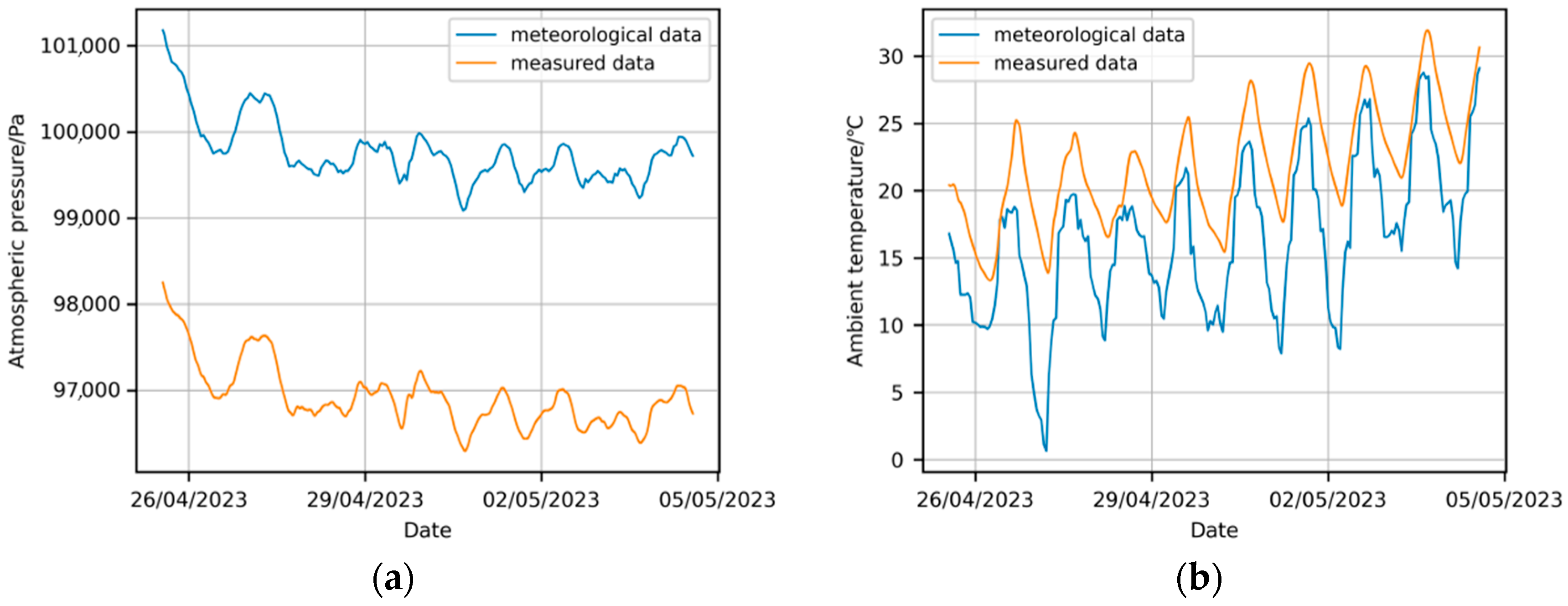
This experiment aims to develop a pressure difference prediction model covering the full flight mission cycle of a stratospheric airship. Due to the absence of subsequent environmental data in the original dataset, meteorological data (atmospheric pressure and temperature with 1 h resolution) from the European Centre for Medium-Range Weather Forecasts (ECMWF), spanning from 25 April to 22 October 2023, was obtained based on the test site coordinates. This data, referred to as meteorological data, was then interpolated to a 10 min time step. A comparison between the actual environmental data from 25 April 2023, 13:25:00 to 4 May 2023, 13:50:00 and the interpolated data revealed a significant discrepancy, as shown in Figure 3.
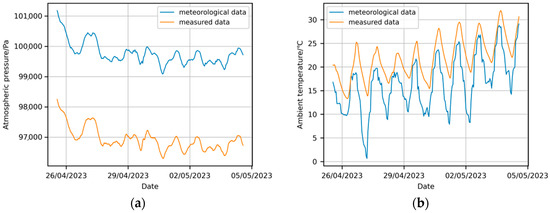
Figure 3.
Comparison of environmental condition data from different sources: (a) comparison of atmospheric pressure; (b) comparison of external gas temperature.
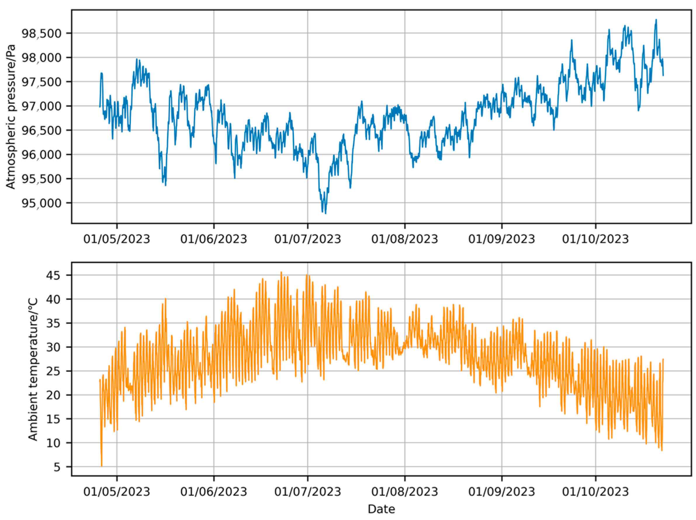
To compensate for the discrepancy between the new environmental data and the measured environmental data, the mean error was applied to adjust the new environmental data. The final corrected environmental condition data variation curve is shown in Figure 4.

Figure 4.
Corrected ECMWF data.
To obtain the pressure difference of the airship envelope under the new environmental conditions, we now proceed with the derivation of the formal. Assuming the leakage behavior of the airship’s envelope is the same under both the experimental field and new environmental conditions, the conditions at the same time point in both environments will follow the ideal gas law (Equation (2)).
where
is the gas pressure;
is the gas volume;
is the gas temperature;
Subscript means this variable is derived from original data;
Subscript means this variable is derived from corrected ECMWF data.
Let atmospheric pressure be and differential pressure be . The internal gas pressure of the airship envelope can be calculated using Equation (3).
Substituting Equation (3) into Equation (2) yields Equation (4).
In the case of the airship envelope being filled with gas, the calculation of the gas volume inside the envelope can be converted to the calculation of the envelope’s volume. To simplify the calculation, the envelope structure is approximated as a cylinder. The formula for the envelope volume calculation is given by Equation (5).
where
represents the constant pi, which is taken as 3.14;
is the actual radius of the airship envelope’s cross-section;
is the simplified length of the envelope.
According to the measured data, the radius and length of the envelope vary with the internal gas pressure. Here, the relationship is simplified using a linear approximation. Let the relationship between the radius and pressure be given by Equation (6), and the relationship between the length and pressure be given by Equation (7).
In these equations, and are the initial radius and length of the chamber, respectively, while and are the linear strain coefficients for the radius and length in response to pressure changes. This approach adjusts empirical pressure differentials to match the corrected ECMWF data, enabling consistent comparative analysis.
The formula for the volume calculation is obtained by combining Equations (5)–(7), as shown in Equation (8).
Substituting Equation (2) into Equation (8) yields Equation (9).
By substituting Equation (9) into Equation (3), a one-variable quartic equation with as the unknown is obtained, as shown in Equation (10).
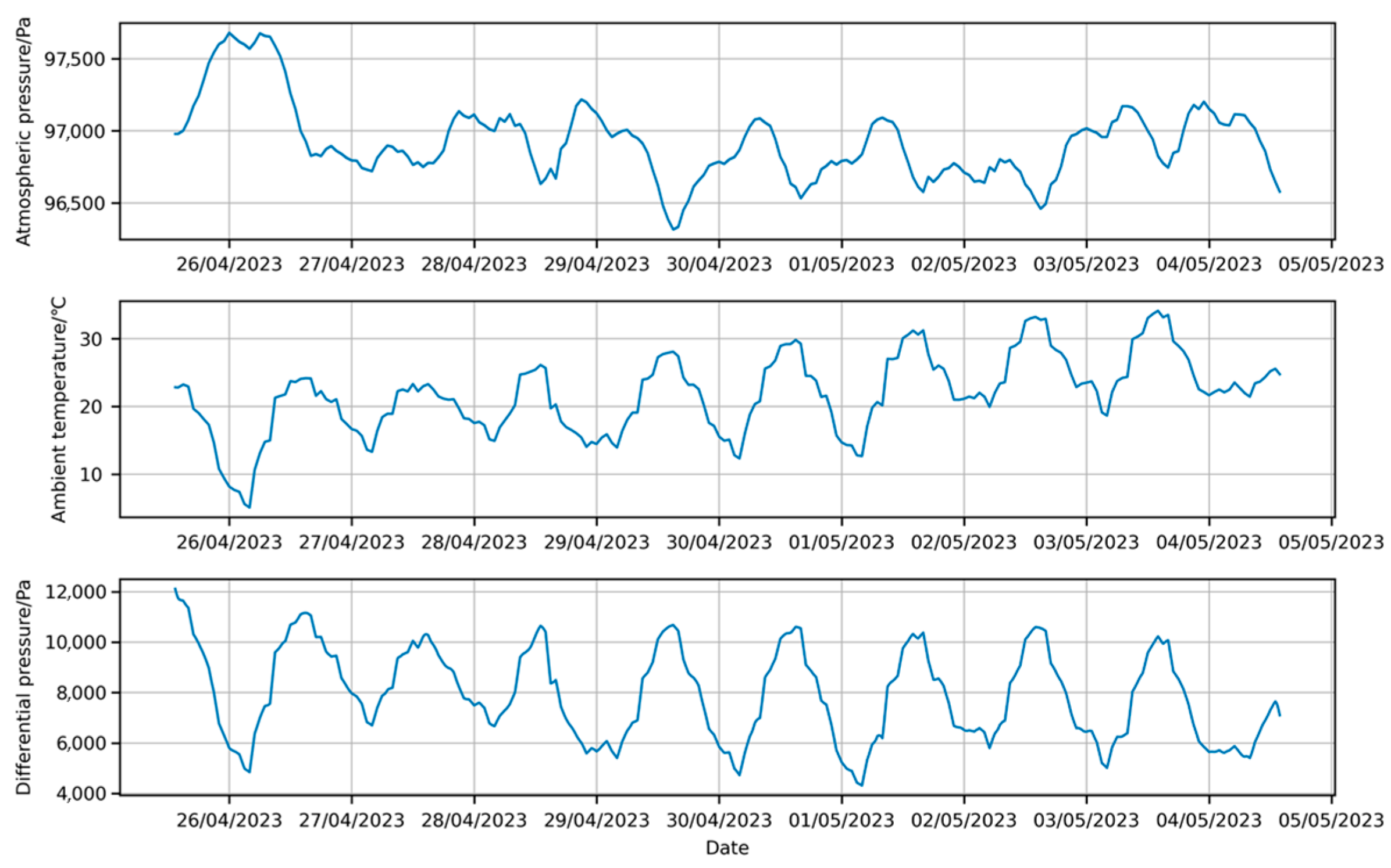
It should be stated that, as shown in Figure 2, the gas temperatures inside and outside the envelope are strongly linearly correlated. Therefore, in the calculations, the environmental temperature data is used to replace the internal gas temperature of the envelope. The final resulting sample set is shown in Figure 5.
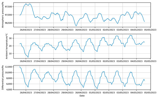
Figure 5.
Sample set.
As shown in the figure above, within the sample set’s time range, both atmospheric pressure and the envelope show a slight decreasing trend, while environmental temperature exhibits a clear increase. The diurnal fluctuations of environmental temperature and envelope pressure difference are nearly synchronized, with aligned phases and coinciding extreme points. In contrast, atmospheric pressure fluctuations do not follow a consistent diurnal pattern of increasing during the day and decreasing at night.
2.2. Sample Partitioning
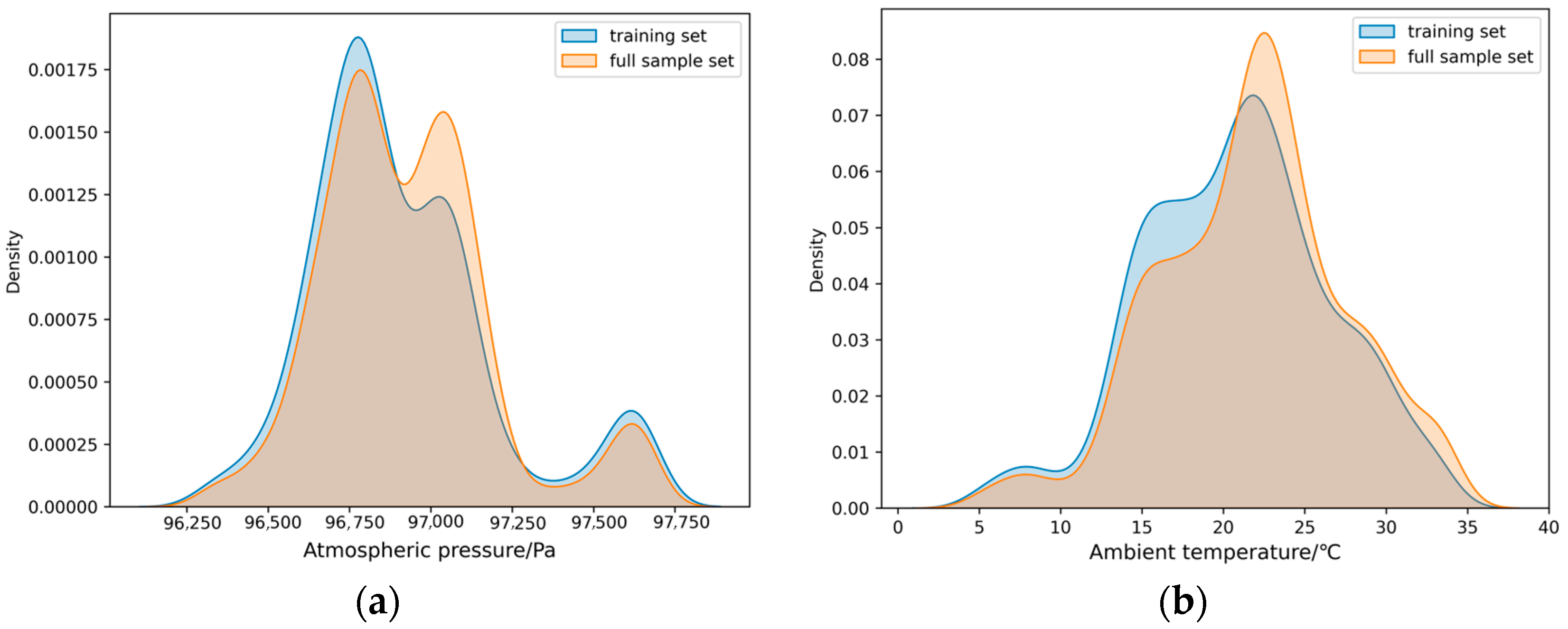
The environmental atmospheric pressure and temperature features in the training set are compared with the corresponding features in the sample set, and a kernel density plot is generated as shown in Figure 6.

Figure 6.
Kernel density estimation: (a) comparison of training set atmospheric pressure and sample set atmospheric pressure data; (b) comparison of training set external gas temperature and sample set external gas temperature data.
The higher the peak of the kernel density plot, the denser the data at that point. Figure 6a shows the distribution difference of atmospheric pressure data between the training set and the full sample set. The training set exhibits a unimodal distribution, while the full sample set shows a bimodal distribution. Figure 6b illustrates the distribution difference of environmental temperature data. Although the kernel density curves have similar widths, the peak for the full sample set is higher, indicating a more concentrated distribution. These differences should be considered when analyzing the prediction results.
3. Evaluation Metrics and Model Selection
This section introduces the evaluation metrics used for the quantitative comparison of prediction results and the experimental models selected.
3.1. Evaluation Metrics Selection
This study evaluates model performance using four metrics: Mean Absolute Error (), Mean Absolute Percentage Error (), Root Mean Square Error (), and the Coefficient of Determination (). Let the data length be , represent the actual data, the predicted values, and represent the mean of the actual data. is the average of the absolute differences between predicted and actual values, calculated as shown in Equation (11).
is used to measure the degree of fit between the fitted curve and the actual data. The calculation formula is shown in Equation (12).
and are expressed in the same units as the actual data. While reflects the average error level, is more sensitive to extreme errors and better captures large discrepancies. Both metrics are influenced by the absolute magnitude of errors. To assess the relative error size, the metric is introduced. is used to measure the relative size of the prediction error with respect to the actual values, and its calculation formula is shown in Equation (13).
reflects the relative error size as a percentage, with smaller values indicating smaller prediction errors. However, is highly sensitive to zero values and can become very large when the actual values approach zero.
The above metrics focus on prediction errors. To intuitively assess the model’s goodness of fit, the Coefficient of Determination () is introduced. The calculation formula is shown in Equation (14).
evaluates the goodness of fit, quantifying how well the model explains the variability in the data. ranges from 0 to 1: a value close to 1 indicates a good fit, with the model explaining most of the variability; a value near 0 suggests the model has little explanatory power and does not capture the data’s variability effectively; and a value less than 0 means the model performs worse than a simple mean model, indicating a poor fit.
In summary, a higher indicates a better fit, while a lower or negative indicates a poor or even worse fit compared to using the mean of the data.
3.2. Model Selection
Due to the large scale of the prediction dataset, traditional statistical models have relatively long computation times. Therefore, this study focuses on traditional machine learning and deep learning methods. The performance of several common models in stratospheric airship envelope airtightness prediction will be compared, as shown in Table 2.
Table 2.
Prediction model selection.
XGBoost, introduced in 2015, is an efficient machine learning method based on the gradient boosting algorithm, widely used in classification and regression tasks, such as species classification, website identification, and index prediction [9,10,11,12]. When analyzing the influence of multiple variables on the prediction target, XGBoost clearly highlights the importance of each variable [13]. Additionally, XGBoost can handle missing values, reducing the data preprocessing workload.
In 2017, Facebook introduced Prophet, a time series analysis tool. Compared to traditional statistical models, Prophet is more user-friendly and does not require extensive statistical or data analysis knowledge. The model accounts for nonlinear trends and seasonal fluctuations and is robust to outliers and missing values [14].
Time series neural networks integrate time series analysis with neural networks, with common types including Recurrent Neural Network (RNN) and Long Short-Term Memory (LSTM). LSTM, a special RNN architecture, mitigates the vanishing gradient problem in long sequences, offering improved generalization. It is widely used in applications such as fault diagnosis, stock prediction, and weather forecasting [15,16,17]. Despite their strong generalization ability, neural networks require large, well-structured datasets to perform optimally. They generalize better when the dataset is well-distributed and there is a high correlation between the training and test sets.
In the LSTM model prediction experiment in Section 4.2.2, Seasonal-Trend decomposition using Loess (STL) decomposition [18] will be used to analyze the results. Time series decomposition breaks down data into interpretable components [19]. For STL decomposition, given the time series data , the decomposition results in trend component , seasonal component , and residual component . This method is simple, computationally efficient, and robust in handling missing and outlier data [20]. In predictive applications, Yang et al. combined STL decomposition with LSTM to create the Decomposed Long Short-Term Memory Network (DLSTM), which improved prediction accuracy by 18% compared to traditional LSTM [21].
Building on Prophet, Facebook introduced the NeuralProphet model, which integrates AR models and time series neural networks. This model offers scalable predictive capabilities and interpretability [22]. It has been widely used in disease prediction. Like Prophet, NeuralProphet includes trend, seasonal, and holiday components, while adding nonlinear deep network components, autoregressive terms, and covariates [23].
Four models were selected for comparison, each with distinct advantages: XGBoost provides efficient baseline predictions; Prophet handles periodicity through decomposable trend and seasonality components [24]; LSTM demonstrates deep learning capabilities; NeuralProphet combines statistical and deep learning approaches. This systematic comparison offers theoretical and practical insights for stratospheric airship envelope permeability prediction.
3.3. Computing Resources
The computational resources utilized in this study are presented in Table 3 below.
Table 3.
Table of computational resource specifications and descriptions.
4. Experiment
The minimum pressure differential of a certain airship’s envelope is 300 Pa. Considering the various loads carried by the envelope, a minimum threshold of 1000 Pa is set. It is necessary to predict whether the envelope’s pressure differential can be maintained above this minimum threshold throughout the sample period.
4.1. Computational Results
Before using neural networks for prediction, mathematical calculation methods are required to assess the airtightness performance of the airship envelope. This assessment will serve as the basis for evaluating the accuracy of the neural network predictions. According to the material specifications for the envelope, the air permeability rate is . Based on the ideal gas law (Equation (15)),
Using the initial pressure differential values from the meteorological data training set, the calculation was performed, and the variation curve of the internal gas pressure differential of the envelope between 25 April 2023 and 22 October 2023 is shown in Figure 7.
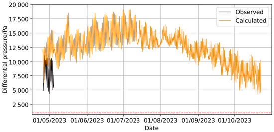
Figure 7.
Curve of envelope pressure difference changes obtained by calculation method.
The calculation results indicate that the envelope’s airtightness meets long-duration flight requirements. However, there is a significant discrepancy between the calculated curve and the pressure differential curve from the sample set (Figure 5). In practical applications, the air permeability of the envelope may vary due to environmental factors such as atmospheric pressure, pressure differential, and the gas temperature both inside and outside the envelope. To improve accuracy, a predictive model will be established based on the sample set.
4.2. Prediction Results
In this section, the same training and testing sets are used to establish the predictive model. The sample set shown in Figure 5 is divided into training and testing sets at an 8:2 ratio.
4.2.1. Evaluation Metrics
The XGBoost, Prophet, LSTM, and NeuralProphet models selected in Section 3.2 were trained using the training set. The performance of the optimized models on the test set is shown in Table 4.
Table 4.
Evaluation of prediction results of models.
As shown in the table above, the XGBoost model performs the best, with all metrics significantly outperforming the other models and demonstrating very low prediction error on the test set. The LSTM and NeuralProphet models perform similarly to XGBoost, with higher and values, but their values are close to 1, indicating that both models can fit the data well and make effective predictions.
The Prophet model exhibits high , , and values, as only reflects the goodness of fit and does not account for error magnitude or prediction uncertainty. Based on these metrics, Prophet performs well in capturing data trends but shows lower accuracy in predicting individual points. Further analysis will focus on the confidence intervals provided by the Prophet model.
In terms of computational efficiency, the XGBoost model demonstrates a significant advantage, being much faster than the other three models. For short-term forecasting tasks, XGBoost maintains optimal performance, followed by LSTM, while NeuralProphet and Prophet are relatively slower. Notably, in long-term forecasting scenarios, NeuralProphet outperforms the other models with a prediction time of 1.30 s. Overall, XGBoost excels in short-term forecasting with high real-time requirements, while NeuralProphet shows better computational efficiency for long-term trend forecasting. The Prophet model is relatively limited in its application due to constraints in both prediction speed and accuracy. Although LSTM performs reasonably well in short-term predictions, its high variance during training suggests room for improvement in stability. These results provide clear guidance for model selection in different application scenarios: XGBoost is recommended for real-time systems, while NeuralProphet is more suitable for medium- and long-term forecasts.
The following section will provide a detailed description of the parameter settings for each prediction model and analyze their performance on the sample set and long-term predictions.
4.2.2. Result Curves
- A.
- Model XGBoost
In XGBoost, Gradient Boosting Decision Trees (GBDT) are used as the fundamental prediction unit of the model. The XGBoost-based predictive model is established using the parameters shown in Table 5.
Table 5.
XGBoost model parameters.
In the table, N_estimators sets the number of GBDT in the model, while Max_depth defines the maximum depth of each GBDT. Subsample controls the proportion of training samples to reduce overfitting, and Colsample_bytree regulates the proportion of features used by the GBDT to prevent overfitting to certain features. Random_state manages the randomness in the training process, ensuring the reproducibility of the experiment.
During the model training process, three input features—environmental atmospheric pressure, temperature, and pressure differential—were selected. Each feature includes the current value, and the lagged values from the past 6 time steps are also incorporated as temporal features. In the sample set, the prediction results are shown in Figure 8. Lag refers to the time offset between the current observation and the observation at a previous time point within the same time series data. Performing a lag of n steps means calculating the difference between the current observation and the observation n time steps earlier.
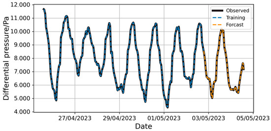
Figure 8.
Prediction of differential pressure changes based on XGBoost.
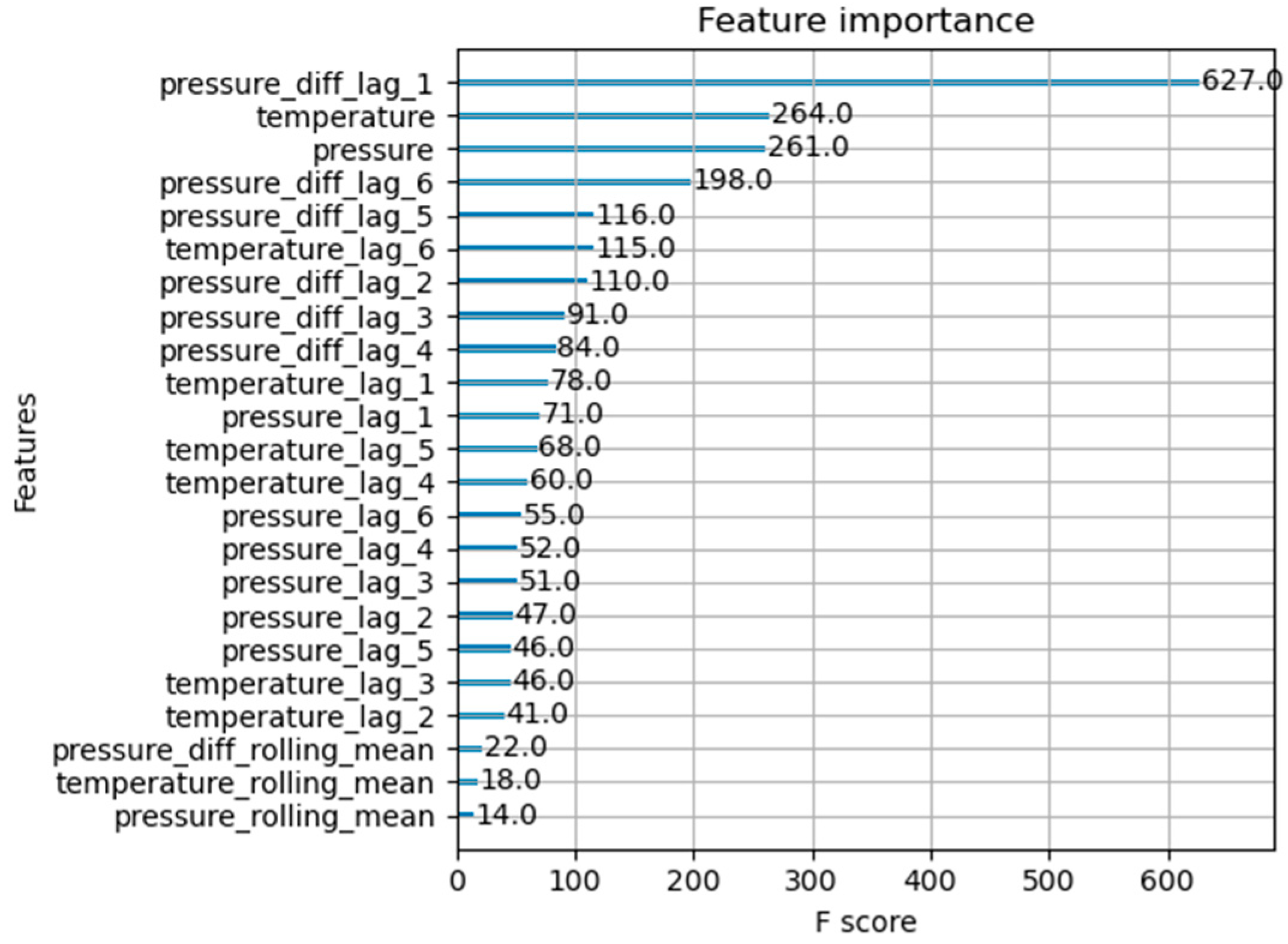
Figure 9 presents the contribution of each input feature to the model’s prediction results.
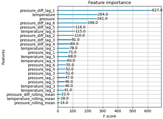
Figure 9.
Output feature importance score.
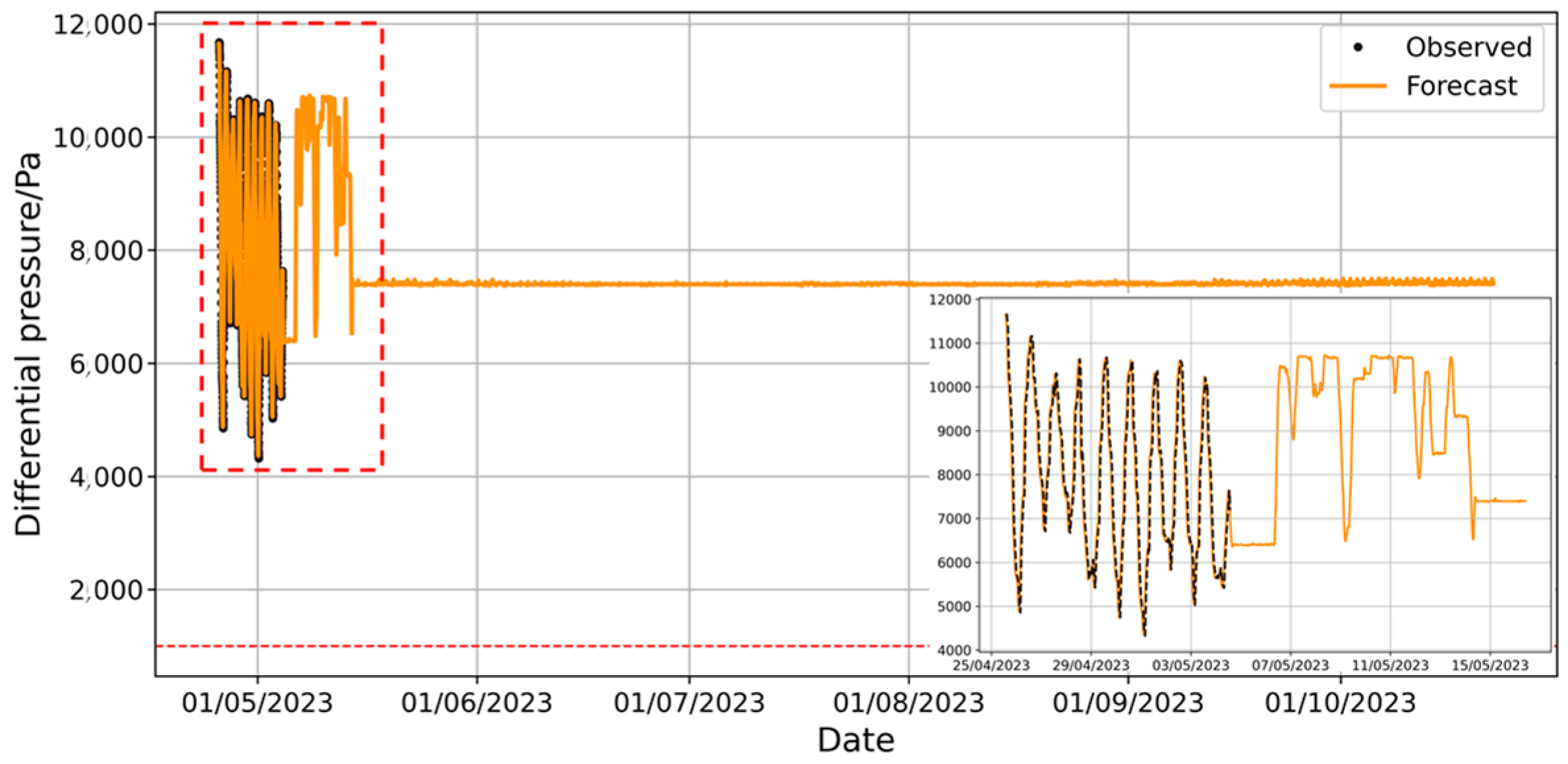
As seen in the figure above, it is clear that the XGBoost model is most influenced by the pressure differential lagged by 1 step. This model is used to predict the long-term changes in the pressure differential inside and outside the capsule. The prediction employs a rolling forecasting approach: the current predicted value is added to the dataset, and the next step is predicted. The prediction results are shown in Figure 10.
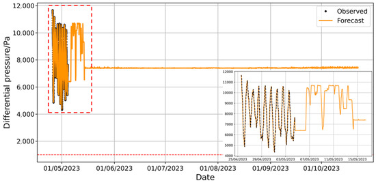
Figure 10.
Prediction of long-term pressure difference changes by XGBoost model.
The results from the figure show that the XGBoost model’s predictions exhibit short-term fluctuations similar to the day–night variation in the sample data. However, as the forecast horizon increases, the amplitude of the pressure difference fluctuations gradually diminishes and eventually approaches a straight line. Clearly, the XGBoost model fails to accurately capture the temporal dependencies in the data during this process. As shown in Figure 5 and Figure 9, the model’s predictions are primarily influenced by the pressure difference lagged by one time step, which leads to cumulative temporal errors in the rolling prediction process: the prediction bias at each time step propagates to the next step, and after several steps of rolling, this error accumulation results in the complete loss of the day–night fluctuation characteristics and the failure of the forecast.
- B.
- Model Prophet
In Prophet, “seasonality” refers to fluctuations or patterns in the data that repeat periodically, typically at specific intervals such as yearly, weekly or daily (Prophet model does not support a parameter for monthly seasonality). To build the Prophet prediction model, Table 6 provides the best parameters.
Table 6.
Prophet model parameters.
In Table 6, Seasonality_mode is used to control the correlation between fluctuations and trends in the model. For this study, it is assumed that the data’s fluctuations are independent of the trend. For the additive modeling Prophet model, the prediction result is calculated as shown in Equation (16).
In this equation, represents the trend component, represents the seasonal component, represents the holiday effect component (which is zero in this model), and represents the error term, accounting for variations that the model cannot capture, assumed to follow a normal distribution. Table 6 indicates that the model captures only daily periodic fluctuations. Holidays assumes that no special holidays or events significantly affect the data. Interval_width defines the width of the uncertainty interval for the forecast results. The Prophet model’s predictions for the sample set are shown in Figure 11, with the shaded area representing the 95% confidence interval (CI).
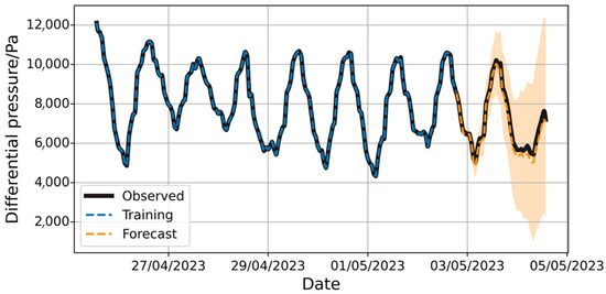
Figure 11.
Prediction of pressure difference changes by Prophet model.
The 95% CI accurately captures the observed values but diverges as the forecast period extends. This indicates a decline in prediction reliability over time. While the CI initially provides a reasonable estimate of uncertainty, its widening suggests that the model’s accuracy decreases for longer forecasts, reducing its practical value for long-term predictions. The composition of the results, including the trend, daily seasonality, and additive regression variables, is shown in Figure 12.
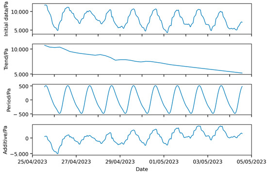
Figure 12.
Components of Prophet model prediction.
As shown in Figure 12, the forecast error of the sample set exhibits an overall downward trend, while the additive regression variables clearly do not follow a normal distribution. These variables exhibit periodic fluctuations and an upward trend corresponding to the day–night cycle, suggesting that the additive regression variables capture temporal dependencies that were not accounted for by the Prophet model. Consequently, the Prophet model was used to forecast the long-term pressure differential variations inside and outside the airship envelope, with the prediction results shown in Figure 13. The model’s result components are presented in Figure 14.
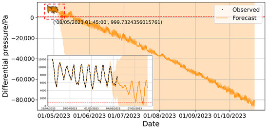
Figure 13.
Prediction of long-term pressure difference changes by Prophet model.

Figure 14.
Components of Prophet model long-term prediction.
By comparing the confidence interval ranges shown in Figure 12 and Figure 13, it is evident that as the prediction time span increases, the confidence interval diverges, eventually becoming so large that it loses its reference value. In long-term predictions, the Prophet model still exhibits significant trend and seasonal characteristics in its additional additive regression variables, which do not follow a normal distribution, indicating systematic bias in the prediction results. Therefore, it is concluded that the additive assumption of the Prophet model is insufficient to capture the underlying patterns in the airship envelope’s airtightness ground test data and is not suitable for this task.
- C.
- Model LSTM
The airtightness prediction based on the LSTM model also adopts a rolling forecast [25]. The model parameters are shown in Table 7.
Table 7.
LSTM model parameters.
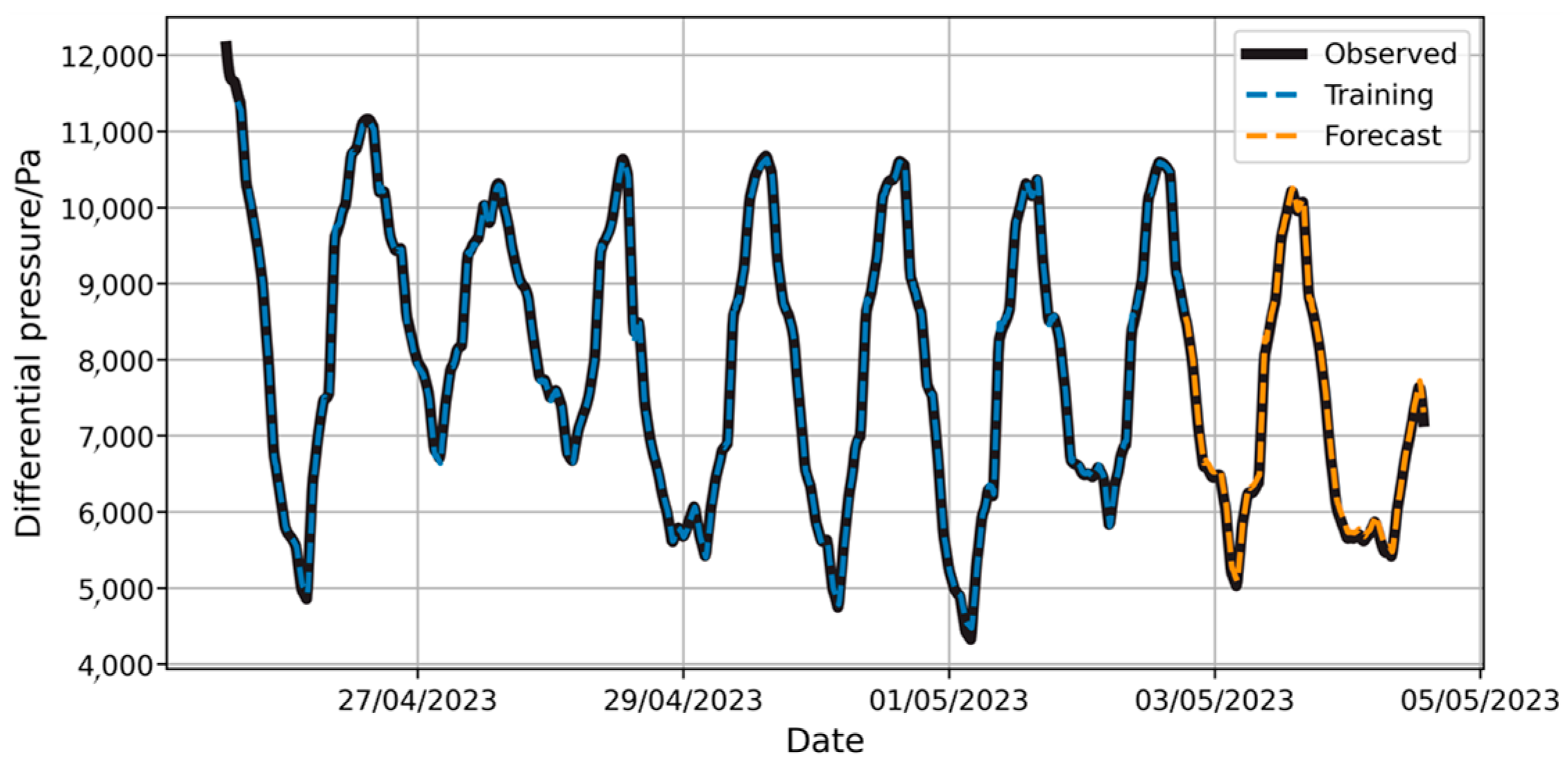
In Table 7, Time step defines the number of time intervals used for each input sequence in temporal models. Hidden size indicates the number of units in the hidden layers of the network, which determines the capacity of the model to learn complex representations. Network layer refers to the number of stacked layers in the architecture, impacting its ability to learn hierarchical features. Learning rate is dynamic, which means it starts at this initial value but can adjust during training to optimize model convergence through adaptive methods. The prediction results are shown in Figure 15.
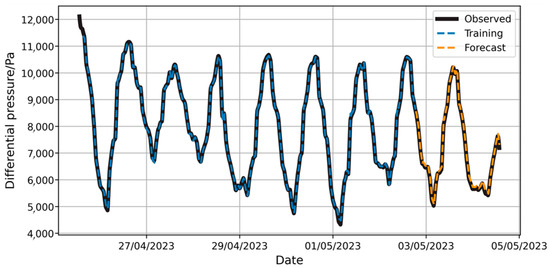
Figure 15.
Prediction of pressure difference changes by LSTM model.
Neural networks typically evaluate model training status and generalization capability by monitoring the training loss and validation loss. For the model in this chapter, the MSE between predicted and actual values is computed after each training epoch as the loss metric, which guides subsequent operations. The target value is established at ; if the model’s validation loss exceeds this upper limit upon training completion, the model is considered to have poor fitting performance. The target value is established at , and training terminates when the validation loss falls below this objective. An automatic learning rate reduction is triggered when the training loss exhibits a monotonically increasing trend for 10 consecutive epochs.
The loss and learning rate changes during the model’s training process are illustrated in Figure 16.
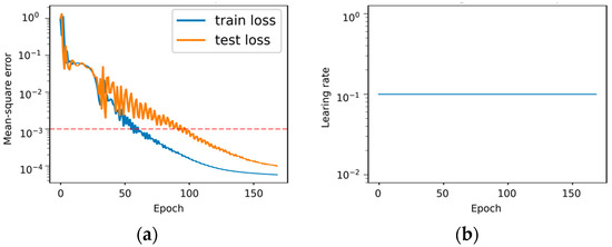
Figure 16.
Changes across training epochs: (a) changes in loss; (b) changes in learning rate.
During the training process, the model’s loss exhibited an overall decreasing trend. However, significant fluctuations occurred around the 50th epoch. The loss decreased below the upper threshold by the 100th epoch and ultimately fell below the target value at approximately the 150th epoch, triggering training termination. The prediction results for long-term forecasting tasks are shown in Figure 17.
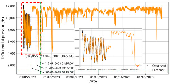
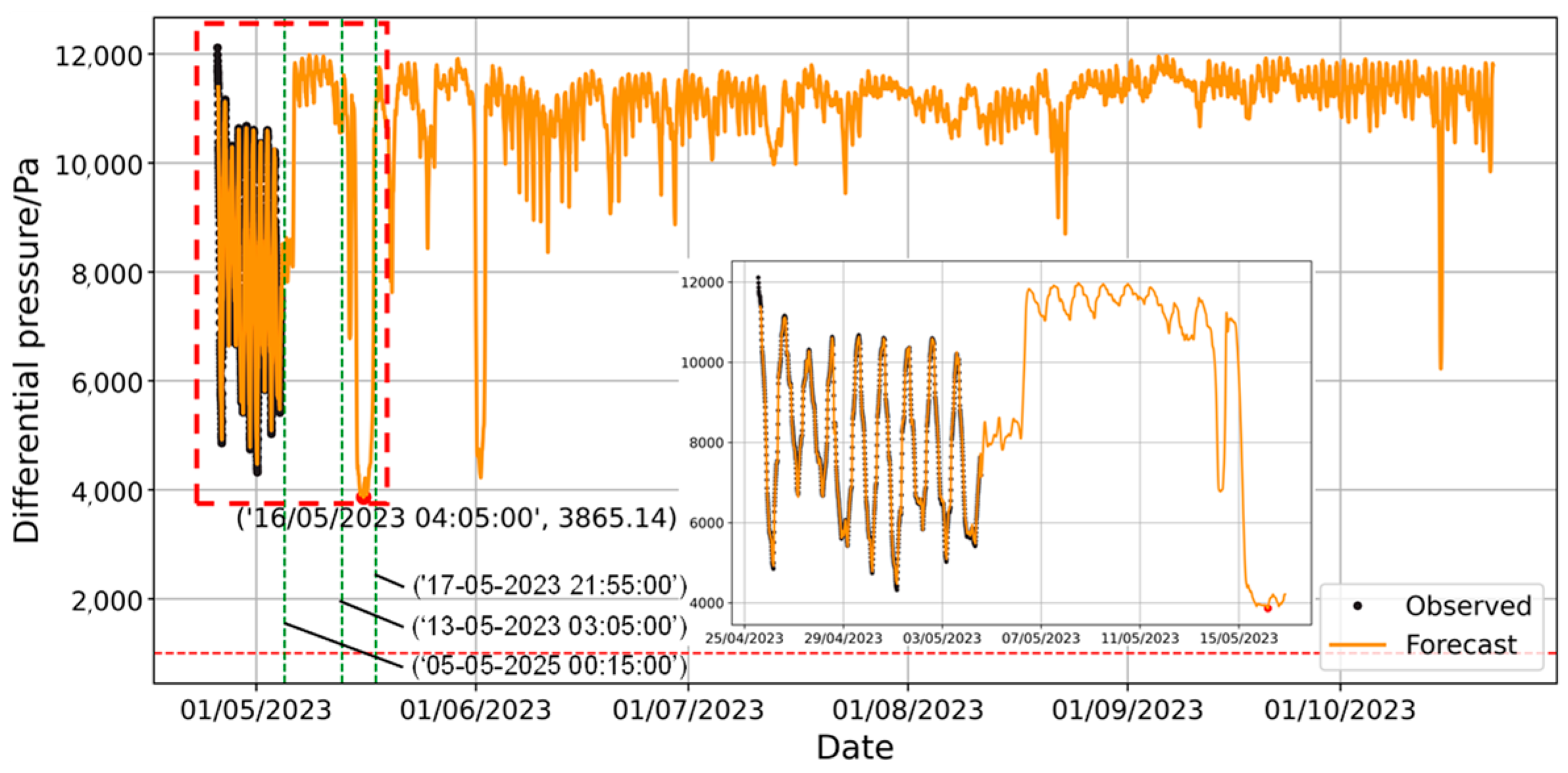
Figure 17.
Prediction of long-term pressure difference changes by LSTM model.
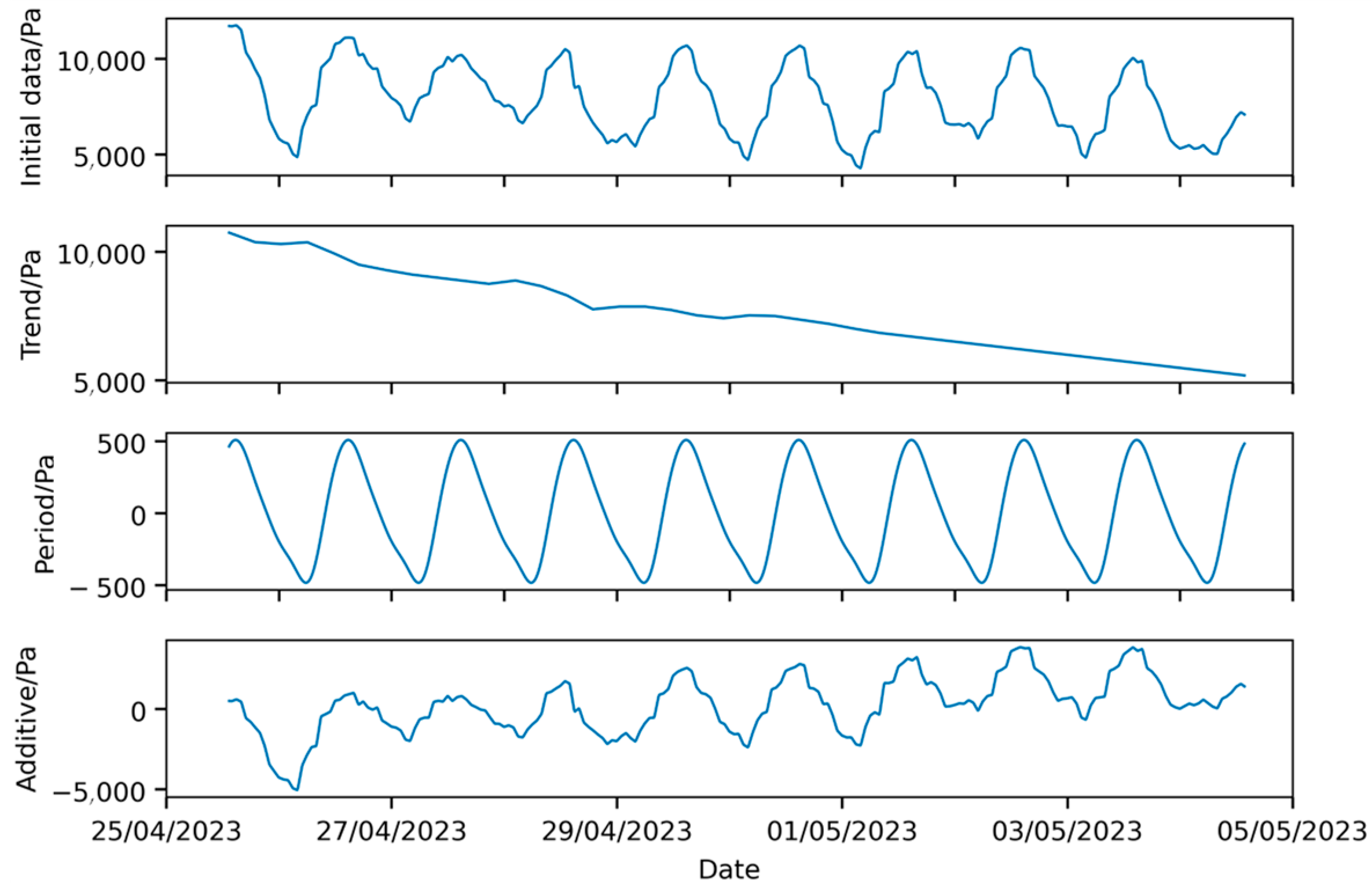
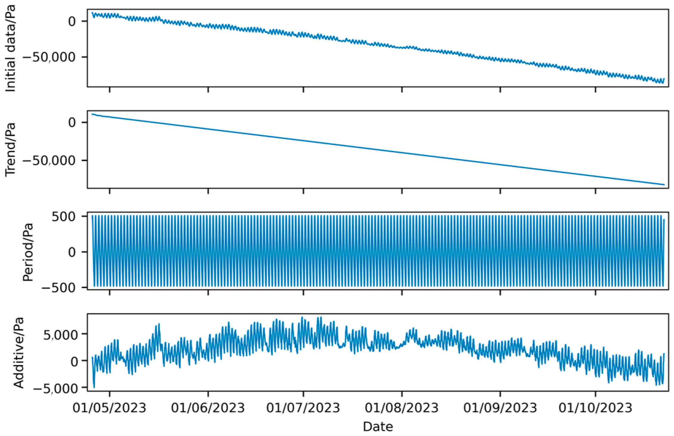
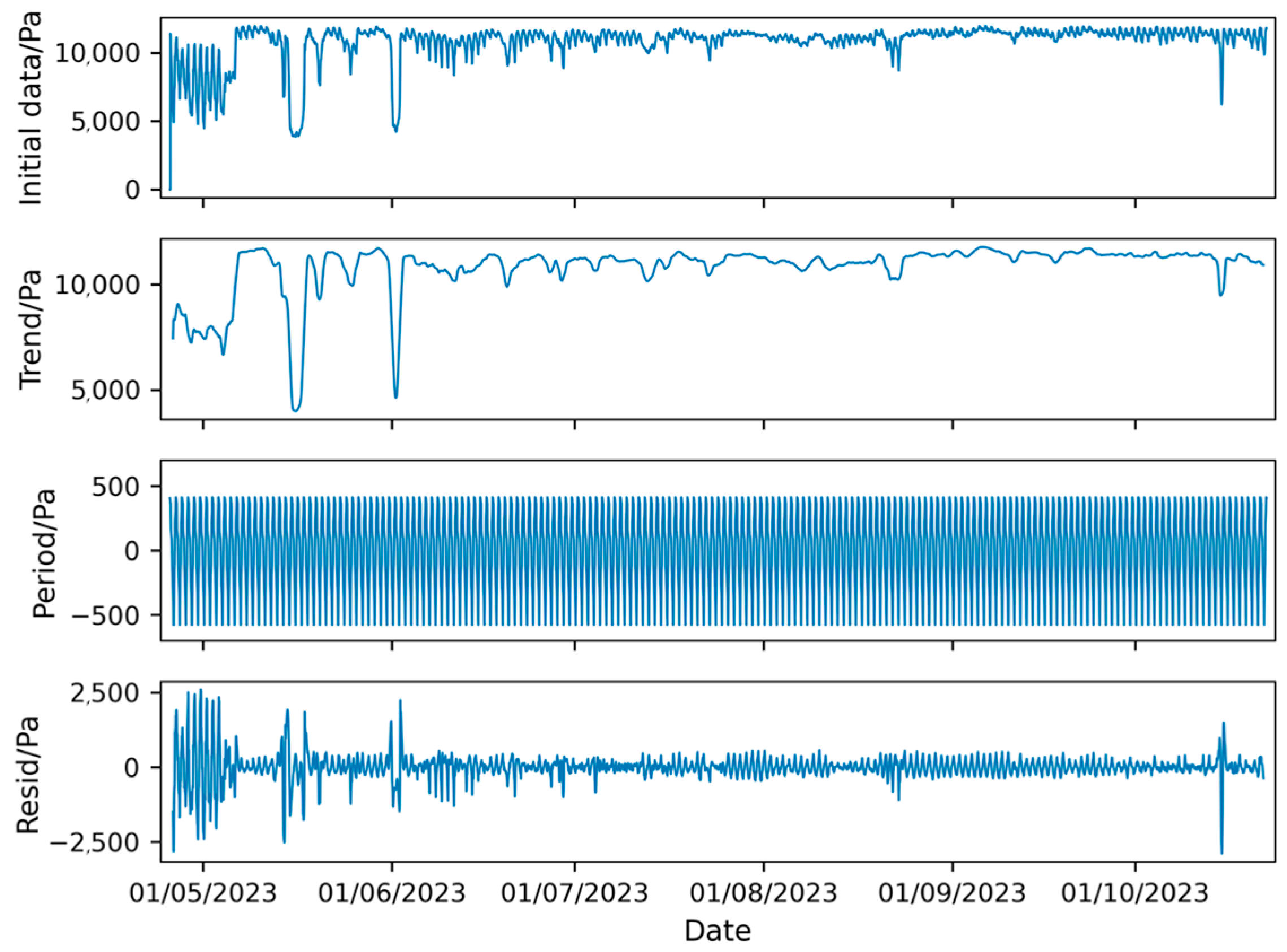
The forecast indicates that the airship envelope pressure differential will remain above 1000 Pa from 25 April 2023 to 22 October 2023, with the minimum predicted pressure differential of 3865.14 Pa occurring at 04:05:00 on 16 May 2023. To provide an intuitive representation of the forecast trend, the seasonal decomposition of the predicted curve using STL decomposition is shown in Figure 18.

Figure 18.
Seasonal decomposition of LSTM model prediction results.
The trend curve in Figure 18 contains significant noise, making it challenging to assess the overall pressure differential trend. A comprehensive analysis of the forecast curve reveals that the diurnal fluctuations in the predicted data are much smaller than those in the observed data, indicating that the model fails to capture the diurnal variation characteristics of the pressure differential with the current training set. Given that the feature distribution in the sample set does not fully align with the training set (Figure 6), it is concluded that the LSTM model is unsuitable for the forecasting requirements in this case. In summary, the interpretability of the LSTM predictions is limited, and it is difficult to analyze the components of the forecast results. When the training dataset is small and there is a distribution shift with the test data, the LSTM model is not applicable.
- D.
- Model NeuralProphet
NeuralProphet is a decomposable time series model that provides components such as trend, seasonality, and autoregression in its output. The parameters for the NeuralProphet prediction model are listed in Table 8.
Table 8.
NeuralProphet model parameters.
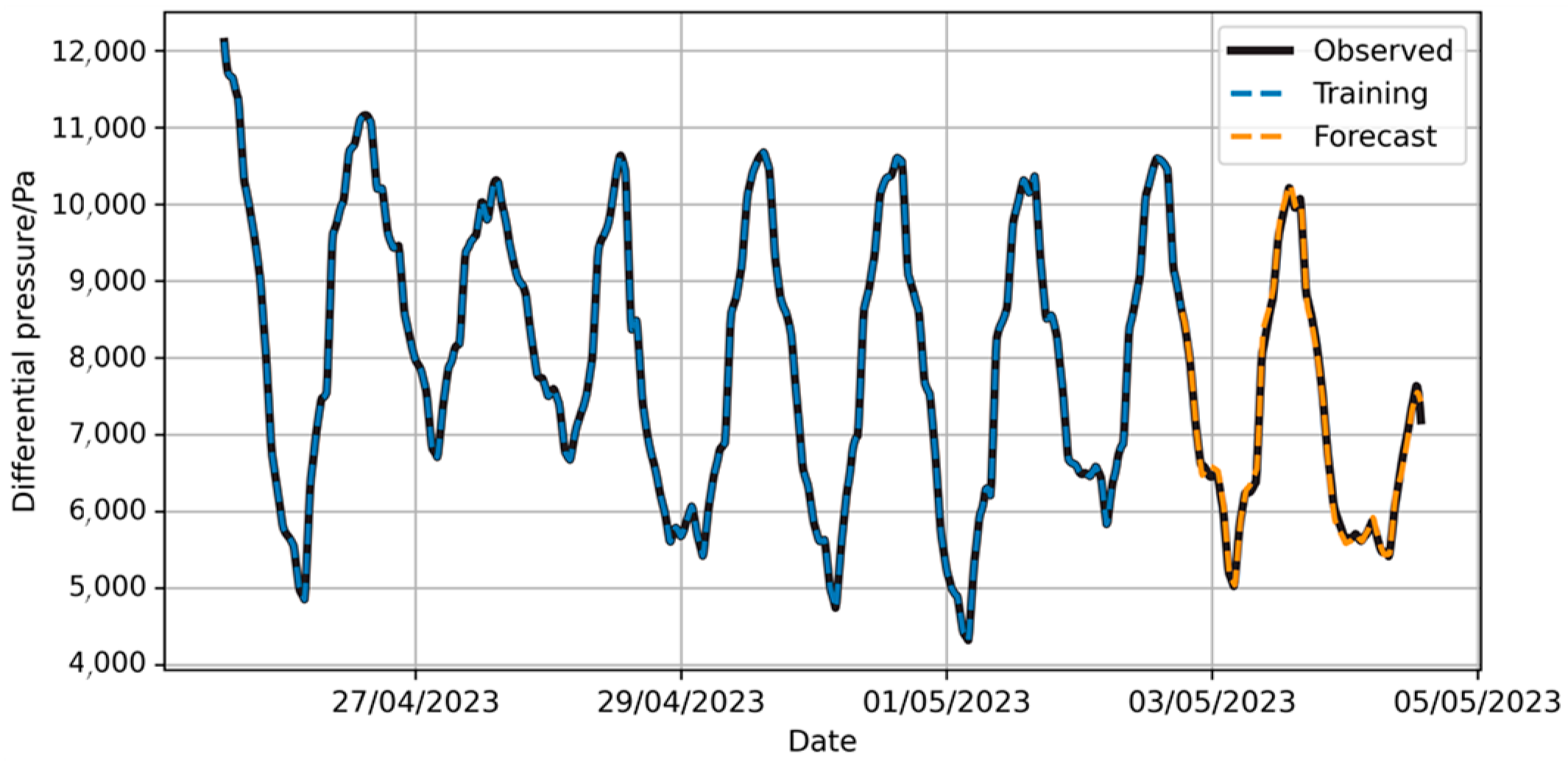
The parameter settings in the NeuralProphet model are similar to those in the Prophet model. The model’s prediction results on the sample set are shown in Figure 19. Long-term prediction results are presented in Figure 20.

Figure 19.
Prediction of pressure difference changes by NeuralProphet model with full training set.
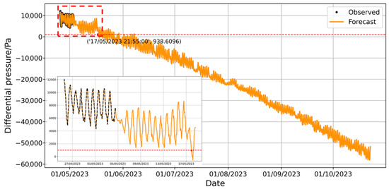
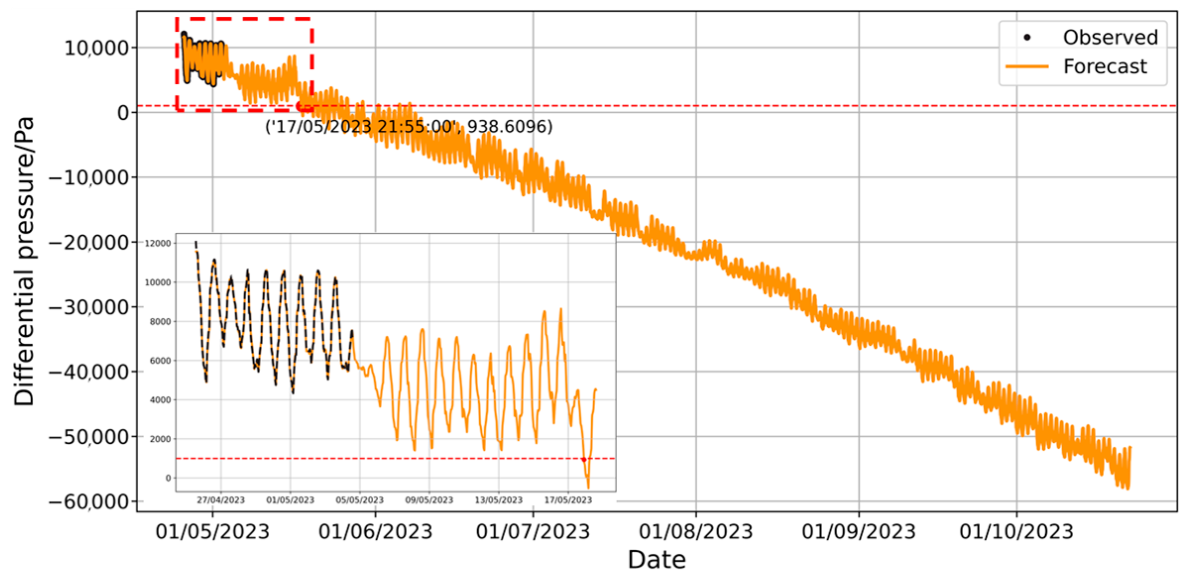
Figure 20.
Prediction of long-term pressure difference changes by NeuralProphet model with full training set.
The prediction results suggest that the pressure differential of the envelope will fall below 1000 Pa at 21:05:00 on 17 May 2023. Upon analyzing the forecast curve, it is observed that the pressure differential decreases significantly after 5 May 2023, which contradicts actual engineering experience. In Figure 4, it is noted that the ambient gas temperature remained stable around 5 May, while atmospheric pressure increased by nearly 1000 Pa thereafter. However, the pressure differential in Figure 20 decreased by nearly 3000 Pa. Even considering potential gas leakage, the original data suggests that a 2000 Pa pressure differential drop between 3 May and 8 May due to leakage is physically implausible. This indicates that the model’s prediction results violate basic physical principles. The model’s output component decomposition is illustrated in Figure 21 [26].
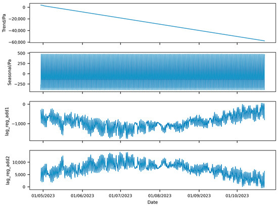
Figure 21.
Component decomposition of prediction of pressure results from NeuralProphet model with full training set.
Examining the trend component of the predicted results in Figure 21 reveals that its slope closely mirrors the pressure differential curve in Figure 5. However, it appears largely unaffected by changes in atmospheric pressure and temperature, suggesting overfitting of the training data. To mitigate the influence of the overall trend of the training set on subsequent predictions, the sample set was divided into a 4:6 ratio for training and testing. The results of this sample set are shown in Figure 22.
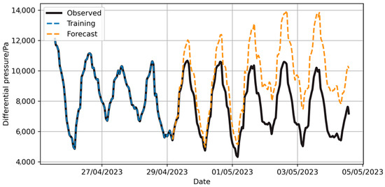
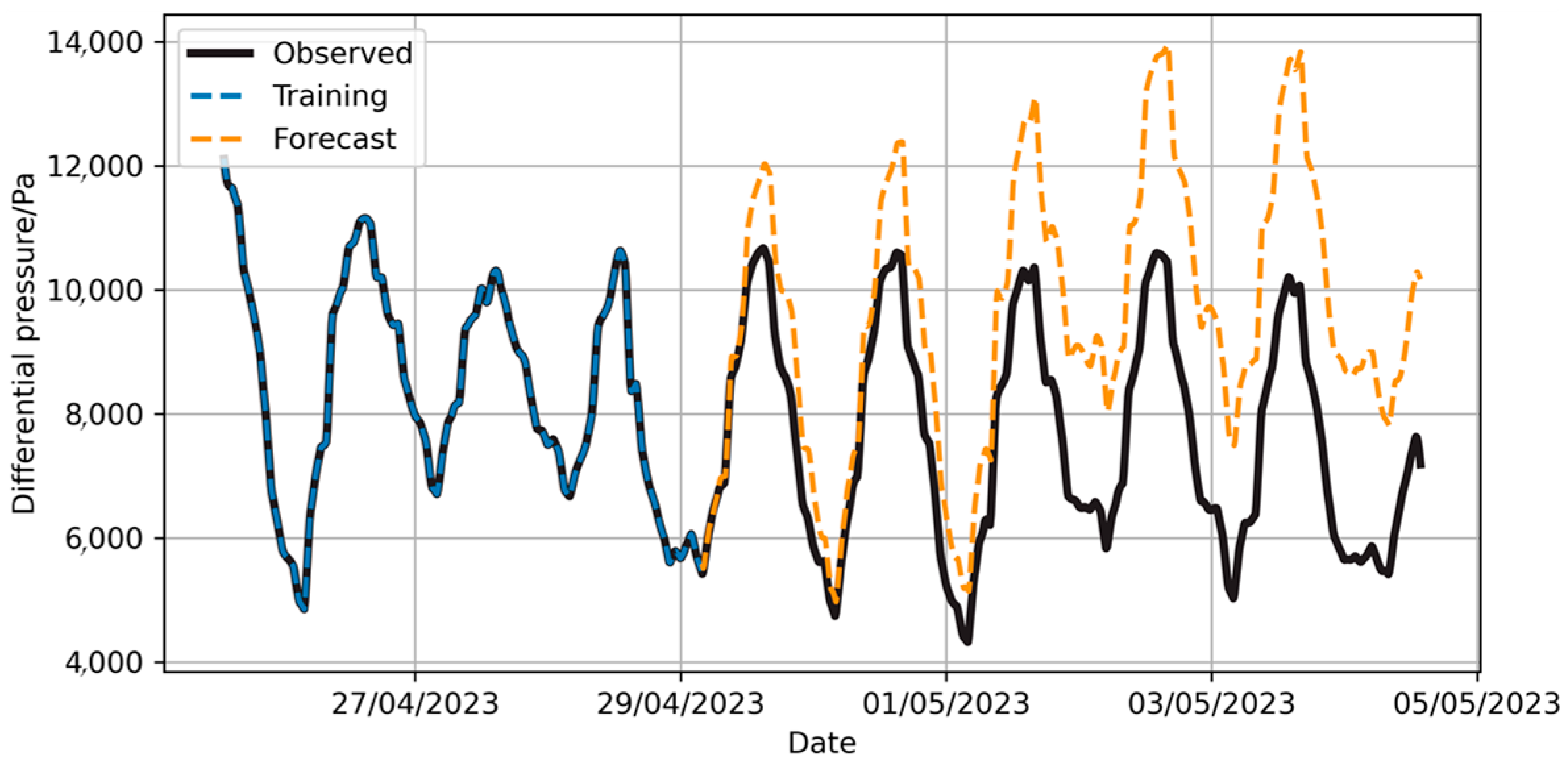
Figure 22.
Prediction of pressure difference changes by NeuralProphet model with reduced training set.
Figure 22 shows that when the size of the training set is reduced to 40% of the total sample set, the model’s prediction results exhibit a clear upward trend, with periodic fluctuation aligning closely with the test set. This concluded that the trend component of the model is less influenced by the data distribution of the sample set. The long-term prediction results of the model are shown in Figure 23, while the component decomposition of the results provided by the NeuralProphet model is illustrated in Figure 24.

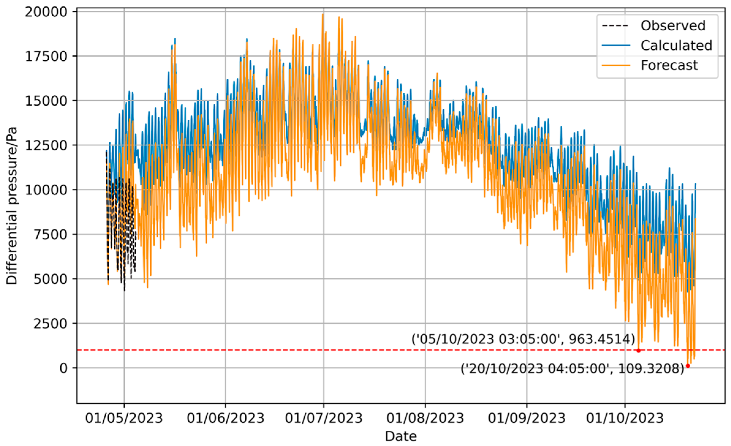
Figure 23.
Prediction of long-term pressure difference changes by NeuralProphet model with reduced training set.

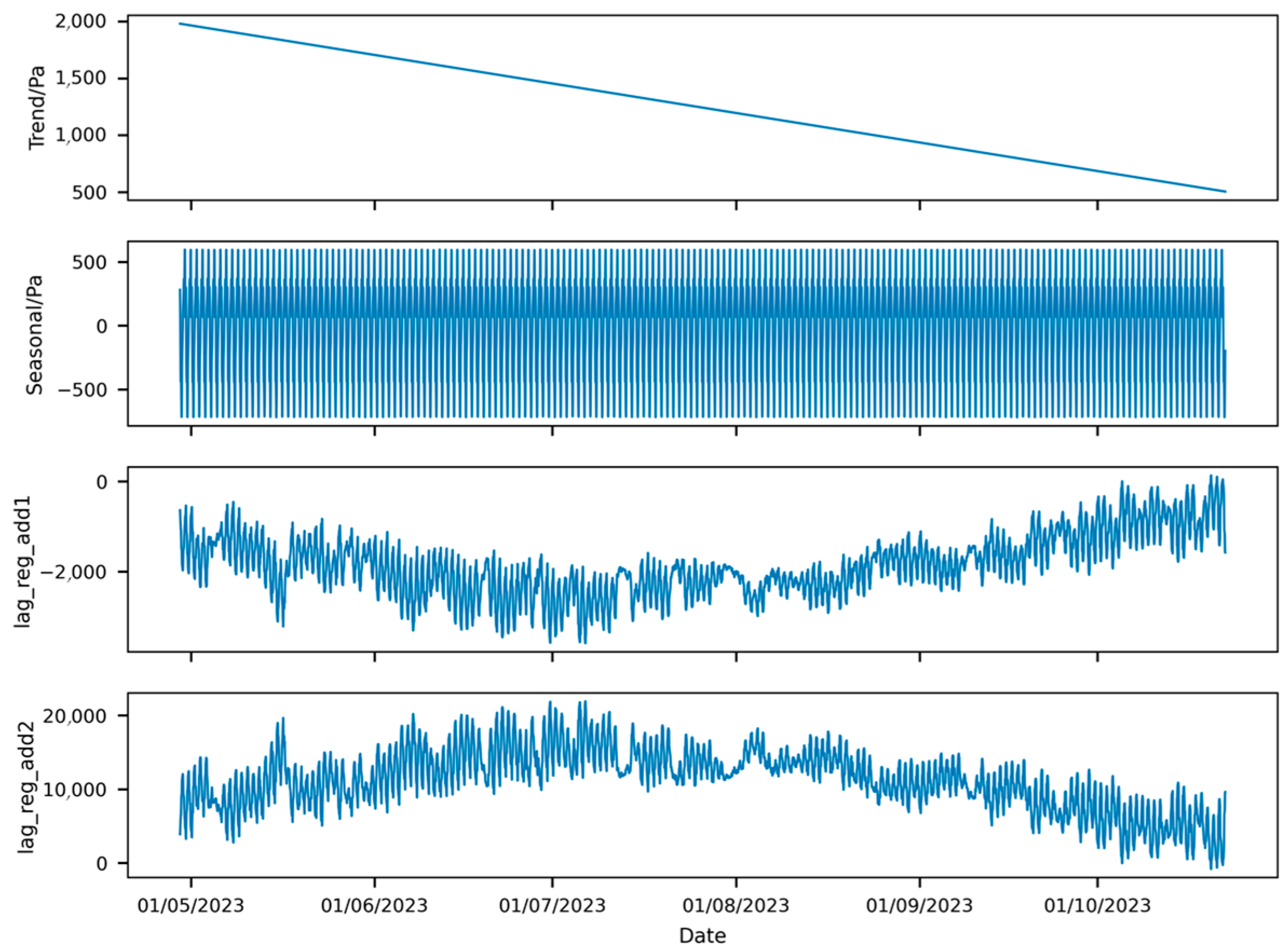
Figure 24.
Component decomposition of prediction of pressure results from NeuralProphet model with reduced training set.
Figure 23 shows that the envelope’s pressure differential is predicted to fall below 1000 Pa at 03:15:00 on 5 October 2023, reaching its lowest value of 91.8 Pa at 04:15:00 on 20 October 2023. Comparing this with the calculated pressure differential curve inside and outside the envelope, the trend and periodic fluctuations of the prediction results from the NeuralProphet model show similarities with the calculated curve, though some discrepancies in the specific numerical values are observed.
Figure 24 shows that the trend component output by NeuralProphet also exhibits a downward trend, though gentler. This is due to the atmospheric pressure drop and the temperature rise from May to July, which increased the pressure differential, partially offsetting the subsequent decrease. In the covariate components, the lag_reg_add1 and lag_reg_add2 terms reflect the influence of atmospheric pressure and external temperature on the pressure differential prediction. Atmospheric pressure has a smaller effect than external temperature. Atmospheric pressure follows the overall trend of the pressure differential, with fluctuations inversely proportional to it, while external temperature exhibits the opposite trend, with directly proportional fluctuation.
Based on the analysis, it can be concluded that under environmental conditions from late April to early November, the airtightness of the airship envelope generally meets operational requirements. Furthermore, it is believed that the NeuralProphet-based prediction model has certain application value in the field of envelope airtightness ground testing.
5. Discussion
In terms of long-term forecasting results from the experiments, it is clear that the current study has several areas for improvement in both the methodological completeness and the innovation of the model, which warrant further exploration.
First, addressing the integration of meteorological data with observational data, it is necessary to develop a dynamic conversion model based on a spatiotemporal attention mechanism. By introducing an adaptive weight allocation algorithm, this model would enable feature-level fusion of multi-source heterogeneous temperature data, thereby effectively expanding the dimensionality of input features and improving data quality.
Second, in the data preprocessing phase, the current approach of directly using ECMWF environmental data lacks rigorous reliability validation. Future work should consider utilizing methods such as the Maximum Information Coefficient (MIC) analysis and spatiotemporal Kriging interpolation for data cleaning, particularly to resolve the phase-matching issue between the temporal resolution of meteorological data and the sampling rate of observational data.
Using MIC, the correlation between multi-source heterogeneous temperature data can be analyzed to fit ECMWF data to the observational data. Spatiotemporal Kriging interpolation can be employed to process ECMWF-derived environmental data, improving the temporal resolution of the data.
Regarding the model architecture, although this study systematically compares the performance of models such as XGBoost, Prophet, LSTM, and NeuralProphet, it has not sufficiently explored three emerging paradigms with significant application potential: first, spatiotemporal forecasting architectures based on Transformer models (such as Informer and Autoformer), whose self-attention mechanisms are particularly well-suited for handling cross-scale correlations between meteorological data and observational data; second, Gaussian Process regression models, which, through kernel function design, can explicitly embed physical constraints such as the gas state equation; third, the recently proposed Kolmogorov–Arnold Networks (KAN), which combine differentiable symbolic regression capabilities to maintain the expressiveness of neural networks (with test set ≥ 0.89) while generating human-readable physical equations (e.g., deriving explicit relationships such as ΔP = α·T + β·RH2). This breakthrough addresses the black-box problem in neural networks.
6. Conclusions
This study employs experimental datasets from stratospheric airship envelope ground-based airtightness tests to develop four time-series prediction models and compare their performance. The proposed approach mitigates the dependency on empirical formulas inherent in traditional computational methods, as well as the complexities associated with model-driven time-series forecasting. This results in improved prediction efficiency within industrial environments, which is crucial for the analysis and evaluation of airship envelope airtightness.
By comparing the performance of each model on the dataset, the study reveals that NeuralProphet demonstrates superior accuracy and fit, particularly in handling the impact of external environmental factors. Compared to other models, NeuralProphet is more effective in capturing the cyclical variations and trends in the data, providing more reliable predictive results in practical applications.
The novelty of this work lies in the application of NeuralProphet to predict the airtightness of stratospheric airship envelopes, a domain that traditionally relied heavily on empirical methods. This study pioneers the use of advanced deep learning models for more accurate and efficient forecasting in complex industrial conditions, particularly those involving dynamic environmental factors.
Therefore, the study concludes that NeuralProphet offers high reliability in predicting the stratospheric airship envelope airtightness ground test dataset, and its application in industrial practices holds significant reference value, particularly for predictive tasks involving complex environmental conditions and dynamic changes, where NeuralProphet exhibits a strong advantage.
Author Contributions
Conceptualization, Y.B. and L.S.; data curation, L.S. and X.Z.; formal analysis, Y.B., L.S. and M.Y.; funding acquisition, W.X.; investigation, Y.B. and L.S.; methodology, Y.B. and L.S.; project administration, W.X. and L.S.; resources, L.S. and X.Z.; software, Y.B.; supervision, L.S.; validation, Y.B. and L.S.; visualization, Y.B.; writing—original draft, Y.B. and M.Y.; writing—review and editing, W.X., L.S. and X.Z. All authors have read and agreed to the published version of the manuscript.
Funding
This research was funded by Major Instrument Project of National Natural Science Foundation of China, 2022YFB3901805. The APC was funded by Aerospace Information Research Institute, Chinese Academy of Sciences.
Data Availability Statement
The data presented in this study are available on request from the corresponding author. Data are not available due to commercial restrictions.
Conflicts of Interest
The authors declare no conflicts of interest.
Abbreviations
The following abbreviations are used in this manuscript:
| ECMWF | European Centre for Medium-Range Weather Forecasts |
| Mean Absolute Error | |
| Mean Absolute Percentage Error | |
| Root Mean Square Error | |
| Coefficient of Determination | |
| LSTM | Long Short-Term Memory |
| STL | Seasonal-Trend decomposition using Loess |
References
- Wasim, M.; Ali, A.; Choudhry, M.; Saleem, F.; Shaikh, I.; Iqbal, J. Unscented Kalman filter for airship model uncertainties and wind disturbance estimation. PLoS ONE 2021, 16, e0257849. [Google Scholar] [CrossRef] [PubMed]
- Shi, Z.; Zhang, X.; Li, J.; Qian, T. The influence of pressure retention index of stratospheric aerostats on their stationary performance. Acta Aeronaut. Et Astronaut. Sinica 2016, 37, 1833–1840. [Google Scholar] [CrossRef]
- Lv, J.; Nie, Y.; Zhang, Y.; Chen, Q.; Gao, H. Research on Environmental Adaptability of Stratospheric Airship Materials. In Man-Machine-Environment System Engineering; Springer: Berlin/Heidelberg, Germany, 2024; Volume 1256. [Google Scholar] [CrossRef]
- Song, L.; Yang, Y.; Zheng, Z.; He, Z.; Zhang, X.; Gao, H.; Guo, X. Theoretical analysis and experimental study on physical explosion of stratospheric airship envelope. Front. Mater. 2023, 9, 1046229. [Google Scholar] [CrossRef]
- Lu, J.; Yang, K.; Zhang, P.; Wu, W.; Li, S. A Trend Forecasting Method for the Vibration Signals of Aircraft Engines Combining Enhanced Slice-Level Adaptive Normalization Using Long Short-Term Memory Under Multi-Operating Conditions. Sensors 2025, 25, 2066. [Google Scholar] [CrossRef]
- Sun, K.; Liu, S.; Gao, Y.; Du, H.; Cheng, D.; Wang, Z. Output power prediction of stratospheric airship solar array based on surrogate model under global wind field. Chin. J. Aeronaut. 2025, 38, 103244. [Google Scholar] [CrossRef]
- Luo, Y.; Zhu, M.; Chen, T.; Zheng, Z. Remaining useful life prediction for stratospheric airships based on a channel and temporal attention network. Commun. Nonlinear Sci. Numer. Simul. 2025, 143, 108634. [Google Scholar] [CrossRef]
- Chen, M.; Liu, Q.; Zhang, J.; Chen, S.; Zhang, C. XGBoost-based Algorithm for post-fault transient stability status prediction. Power Syst. Technol. 2020, 44, 1026–1034. [Google Scholar] [CrossRef]
- Chen, T.; Guestrin, C. XGBoost: A scalable tree boosting system. In Proceedings of the 22nd ACM SIGKDD International Conference on Knowledge Discovery and Data Mining, New York, NY, USA, 13 August 2016; pp. 785–794. [Google Scholar] [CrossRef]
- Xu, Y.; Zhen, J.; Jiang, X.; Wang, J. Mangrove species classification with UAV-based remote sensing data and XGBoost. Natl. Remote Sens. Bull. 2021, 25, 737–752. [Google Scholar] [CrossRef]
- Li, H. Research on Web Spam Detection Method Based on XGBoost Algorithm. Master’s Thesis, Southwest Jiaotong University, Chengdu, China, 2020. [Google Scholar]
- Baghbani, A.; Kiany, K.; Abuel-Naga, H.; Lu, Y. Predicting the Compression Index of Clayey Soils Using a Hybrid Genetic Programming and XGBoost Model. Appl. Sci. 2025, 15, 1926. [Google Scholar] [CrossRef]
- Yin, C.; Ge, Y.; Chen, W.; Wang, X.; Shao, C. The Impact of the Urban Built Environment on the Carbon Emissions of Rede-Hailing Based on the XGBoost Model; Journal of Beijing Jiaotong University: Beijing, China, 2025. [Google Scholar]
- Taylor, S.; Letham, B. Forecasting at scale. Am. Stat. 2018, 72, 37–45. [Google Scholar] [CrossRef]
- Zhu, Y.; Liu, Z. A Dual-Dimension Convolutional-Attention Module for Remaining Useful Life Prediction of Aeroengines. Aerospace 2024, 11, 809. [Google Scholar] [CrossRef]
- Peng, Y.; Liu, Y.; Zhang, R. Modeling and analysis of stock price forecast based on LSTM. Comput. Eng. Appl. 2019, 55, 209–212. [Google Scholar] [CrossRef]
- Hasan, M.M.; Hasan, M.J.; Rahman, P.B. Comparison of RNN-LSTM, TFDF and stacking model approach for weather forecasting in Bangladesh using historical data from 1963 to 2022. PLoS ONE 2024, 19, e0310446. [Google Scholar] [CrossRef]
- Krake, T.; Klötzl, D.; Hägele, D.; Weiskopf, D. Uncertainty-Aware Seasonal-Trend Decomposition Based on Loess. IEEE Trans. Vis. Comput. Graph. 2025, 31, 1496–1512. [Google Scholar] [CrossRef]
- Cao, D.; Ma, J.; Sun, L.; Ma, N. A Time-series Prediction Algorithm Based on a Hybrid Model. Recent Adv. Comput. Sci. Commun. 2023, 16, 3–17. [Google Scholar] [CrossRef]
- Wang, M.; Meng, Y.; Sun, L.; Zhang, T. Decomposition combining averaging seasonal-trend with singular spectrum analysis and a marine predator algorithm embedding Adam for time series forecasting with strong volatility. Expert Syst. Appl. 2025, 274, 126864. [Google Scholar] [CrossRef]
- Yang, J.; Liu, C.; Pan, J. Deformation prediction of arch dams by coupling STL decomposition and LSTM neural network. Appl. Intell. 2024, 54, 10242–10257. [Google Scholar] [CrossRef]
- Triebe, O.; Hewamalage, H.; Pilyugina, P.; Laptev, N.; Bergmeir, C.; Rajagopal, R. NeuralProphet: Explainable Forecasting at Scale. arXiv 2021. [Google Scholar] [CrossRef]
- Pragalathan, J.; Schramm, D. Comparison of SARIMA, Fb-Prophet and NeuralProphet Models for Traffic Flow Predictions at a Busy Urban Intersection. In Technologies for Sustainable Transportation Infrastructures; Springer: Berlin/Heidelberg, Germany, 2024; Volume 529, pp. 127–143. [Google Scholar] [CrossRef]
- Arslan, S. A hybrid forecasting model using LSTM and Prophet for energy consumption with decomposition of time series data. PeerJ Comput. Sci. 2022, 8, e1001. [Google Scholar] [CrossRef]
- Yuan, S.; Wang, C.; Mu, B.; Zhou, F.; Duan, W. Typhoon intensity forecasting based on LSTM using the rolling forecast method. Algorithms 2021, 14, 83. [Google Scholar] [CrossRef]
- Huang, L.; Wu, H.; Lou, Y.; Zhang, H.; Liu, L.; Huang, L. Spatiotemporal Analysis of Regional Ionospheric TEC Prediction Using Multi-Factor NeuralProphet Model under Disturbed Conditions. Remote Sens. 2023, 15, 195. [Google Scholar] [CrossRef]


Disclaimer/Publisher’s Note: The statements, opinions and data contained in all publications are solely those of the individual author(s) and contributor(s) and not of MDPI and/or the editor(s). MDPI and/or the editor(s) disclaim responsibility for any injury to people or property resulting from any ideas, methods, instructions or products referred to in the content. |
© 2025 by the authors. Licensee MDPI, Basel, Switzerland. This article is an open access article distributed under the terms and conditions of the Creative Commons Attribution (CC BY) license (https://creativecommons.org/licenses/by/4.0/).