A Fusion of Deep Learning and Time Series Regression for Flood Forecasting: An Application to the Ratnapura Area Based on the Kalu River Basin in Sri Lanka

Abstract

Flooding is the most frequent natural hazard that accompanies hardships for millions of civilians and substantial economic losses. In Sri Lanka, fluvial floods cause the highest damage to lives and properties. Ratnapura, which is in the Kalu River Basin, is the area most vulnerable to frequent flood events in Sri Lanka due to inherent weather patterns and its geographical location. However, flood-related studies conducted based on the Kalu River Basin and its most vulnerable cities are given minimal attention by researchers. Therefore, it is crucial to develop a robust and reliable dynamic flood forecasting system to issue accurate and timely early flood warnings to vulnerable victims. Modeling the water level at the initial stage and then classifying the results of this into pre-defined flood risk levels facilitates more accurate forecasts for upcoming susceptibilities, since direct flood classification often produces less accurate predictions due to the heavily imbalanced nature of the data. Thus, this study introduces a novel hybrid model that combines a deep leaning technique with a traditional Linear Regression model to first forecast water levels and then detect rare but destructive flood events (i.e., major and critical floods) with high accuracy, from 1 to 3 days ahead. Initially, the water level of the Kalu River at Ratnapura was forecasted 1 to 3 days ahead by employing a Vanilla Bi-LSTM model. Similarly to water level modeling, rainfall at the same location was forecasted 1 to 3 days ahead by applying another Bi-LSTM model. To further improve the forecasting accuracy of the water level, the forecasted water level at day t was combined with the forecasted rainfall for the same day by applying a Time Series Regression model, thereby resulting in a hybrid model. This improvement is imperative mainly because the water level forecasts obtained for a longer lead time may change with the real-time appearance of heavy rainfall. Nevertheless, this important phenomenon has often been neglected in past studies related to modeling water levels. The performances of the models were compared by examining their ability to accurately forecast flood risks, especially at critical levels. The combined model with Bi-LSTM and Time Series Regression outperformed the single Vanilla Bi-LSTM model by forecasting actionable flood events (minor and critical) occurring in the testing period with accuracies of 80%, 80%, and 100% for 1- to 3-day-ahead forecasting, respectively. Moreover, overall, the results evidenced lower RMSE and MAE values (<0.4 m MSL) for three-days-ahead water level forecasts. Therefore, this enhanced approach enables more trustworthy, impact-based flood forecasting for the Rathnapura area in the Kalu River Basin. The same modeling approach could be applied to obtain flood risk levels caused by rivers across the globe.

1. Introduction

Fluvial floods occur when the water level in a river, lake, or stream rises due to excessive rain or snowmelt, submerging neighboring land in a mostly dry state. Since 2000, floods have been accountable for 39% of the natural disasters that have happened worldwide [1]. By 2022, the global impact of flooding accounted for more than 54 million victims, causing the deaths of approximately 7400 people [2]. Being a hazardous natural disaster, flooding has resulted in the highest number of fatalities compared to any other disaster type [3]. The impacts of climate change, rapid population growth, rising sea levels, the poor maintenance of drainage systems, and development activities such as urbanization, land use changes, deforestation, and infrastructure development in river basins are the most common reasons for the severe increase in flooding [4,5,6,7,8].

The complete control of flooding is unachievable due to its chaotic nature. Therefore, flood preparedness is the most effective approach to mitigating damage due to floods. Better flood preparedness can be achieved through forecasting flood occurrences with a considerable time gap [3,9,10,11]. When conducting flood forecasting, obtaining accurate forecasts, especially for flash flood events and major floods, is considered a crucial aspect of both hydrology and disaster management [12].

Flood forecasting is conducted using several methods that come under hydraulic, hydrologic, traditional statistical, machine learning, or deep learning modeling categories (e.g., [3,9,10,13,14,15,16,17,18,19,20,21,22,23,24,25,26,27,28,29,30,31,32,33,34,35]). Some studies have experimented with ensemble modeling and gained better performance levels (e.g., [16,17,19,36]). This is because obtaining accurate forecasts for weather-related phenomena, especially capturing extreme events (e.g., extreme rainfall, flash floods), may not be achievable with a single (or pure) modeling technique [37].

Research studies that model flood occurrence using classification methods are very rare (e.g., [14,15,19]). This is due to the substantial class imbalance resulting from the varying intensities of flood levels. Therefore, most flood-related studies have been conducted to forecast water levels or the discharge/streamflow of rivers that are vulnerable to floods (e.g., [3,18,21,22,24,35]). However, discharge- or streamflow-based forecasting may lead to erroneous flood warnings because of the conversion of data [24]. Therefore, to obtain trustworthy flood forecasts, first the water level of a particular river basin should be modeled, and then the risk levels must be identified based on pre-defined cut-off values for flood risk levels.

Flood forecasting models consist of a vast set of spatiotemporal weather–meteorological predictor variables. The water levels or discharge of neighboring stations, their topographical information, rainfall intensity, soil moisture, and river elevation are the most prominent among them [11,12,13,14,15,16,17,18,19,20,21,22,23,24]. In order to reduce model complexity, the selection of the best set of predictor variables and their significant past lags (i.e., historical window size) is also imperative [38]. Moreover, many studies underscore the fact that adequate flood preparedness requires forecasts of such events at least 3 to 15 (extremely satisfactory) days in advance. [1,11,14].

Heavy or extreme rainfall on a particular day triggers a sudden rise in water levels [38]. Therefore, flood forecasts generated several days in advance must be subsequently updated using rainfall forecasts corresponding to these future days. However, the cruciality of an accurate rainfall forecast before forecasting a flood has been identified by a limited number of hydrological studies (e.g., [19,23,34,39]).

Conventional studies have used the Time Series Data Mining approach (TSDM), which involves statistical tools such as the Autoregressive (AR) model, K-Nearest Neighbor (KNN), and K-means clustering (e.g., [13,14,15]). Study [13] did not report the accuracy of its flood model. In study [14], flood warnings were issued more than five days in advance based on precipitation classification. Although it captures over 90% of extreme precipitation events, not all such events necessarily lead to severe flooding. The TSDM classification model introduced in [15] includes a station-specific parameter selection step before forecasting flood events. Study [19] issued flood warnings based on rainfall event (class) forecasts. However, an accurate flood warning system often depends on a water level forecasting model.

Studies using hydraulic or hydrologic models mainly focus on inundation mapping and satellite image analysis (e.g., [16,17]), along with several topographical characteristics of the river basin (e.g., river-cross section, land cover, and elevation data). These models, which give longer lead times and lower error rates (e.g., [17]), should be tested for generalizability over extended periods.

Traditional methods like TSDM cannot capture the complex relationships between geophysical variables. They are also more prone to producing highly inaccurate predictions when dealing with nonstationary data, missing values, and the unavailability of important weather-related variables. In such cases, machine learning and deep learning (ML and DL) methods have shown to be promising and efficient tools [19,20,23].

Among the studies that use ML, many applied Artificial Neural Network (ANN), Support Vector Machine (SVM), or Support Vector Regression (SVR) (e.g., [3,18,21,24]) approaches. Study [18] compared a SVM and ANN for modeling daily water levels. Studies [3,21,24], which used ANN, SVR, and Neurofuzzy methods, respectively, modeled the hourly river stage (i.e., water level) or river flow and produced short-term flood forecasts, usually a few hours ahead (<7 h). However, this short lead time is usually insufficient for efficient flood preparedness. These studies mainly utilized rainfall and water level/discharge data for flood modeling. Study [3] emphasized that a hybrid approach combining ANN with Fuzzy computing produced better forecasts with longer lead times compared to using a single model alone. The effectiveness of hybrid flood models in improving forecasting accuracy was further highlighted in [20,23].

Compared to ML methods, DL allows the use of long-time lags (i.e., sequential inputs of past lags) when making multi-step-ahead forecasts. Moreover, these methods are well-suited to handling the chaotic and dynamic nature of time series data [19]. The flood modeling in studies [19,20,22,29,30,35] used numerous variants of LSTM such as Smoothing-LSTM (ES-LSTM), Bidirectional LSTM (Bi-LSTM), Conv-LSTM, Stacked LSTM, Vanilla LSTM, and Encoder–Decoder Double-Layer LSTM (ED-DLSTM) for modeling flood occurrence or river discharge. Although these studies demonstrated the strong performance of their LSTM models (e.g., [20]) in both long and short-term flood forecasting, they pay limited attention to explaining forecasting accuracy across different forecasting horizons and to the generalizability of results. Notably, the urban flood forecasting and alerting model in study [33] showed that Bi-LSTM outperformed the other models used in the study, including an ANN and Stacked LSTM.

In general, the existing studies on flood forecasting have several common limitations. These limitations include difficulty in capturing rapid rises in water level (e.g., [39,40]), reliance on a limited set of predictors, a narrow focus on rainfall forecasting, shorter forecasting horizons or lead times (e.g., [41]), performance evaluation using a single metric, difficulty in generalizing their results, a lack of details on deployment strategies, and dependence on a single model which may lead to false predictions [19]. Therefore, our study aimed to address these existing research gaps by

(i)

Employing variants of the LSTM model (i.e., Vanilla and Stacked Bi-LSTM) to forecast future water levels (the basis for this selection was set by studies [33,38] evidencing accurate flood forecasting and the capture of extreme events, respectively);

(ii)

Incorporating rainfall and water level data as predictors after applying better filtering methods (e.g., Granger Causality and cross-correlation tests [38,42]);

(iii)

Generating multiple-days-ahead forecasts for reliable flood preparedness;

(iv)

Introducing a novel hybrid model which further enhances the water level forecasts obtained from LSTM models by incorporating three-days-ahead rainfall forecasts obtained from our previous study [38];

(v)

Conducting residual analysis and modeling to further improve the water level forecasts;

(vi)

Applying the proposed hybrid methodology to a flood-prone river basin located in Sri Lanka.

Floods are recognized as a major destructive natural disaster in Sri Lanka due to the country’s unique climatological and geographical conditions [32]. Every 2 to 3 years, the country experiences a flash flood event, affecting around 200,000 civilians [33]. Sri Lanka has 103 major river basins, of which 17 (such as Kalu, Kelani, and Nilwala) rivers are particularly vulnerable to flooding. Some existing flood warning systems do not function properly. Furthermore, the recently introduced Real-Time Water Level Monitoring Application measures the current water levels of vulnerable rivers and can only issue flood warnings a few hours before an event [9,33,43]. Therefore, there is a clear need for the development of an effective flood forecasting and warning system in Sri Lanka. This study focuses on the Kalu River Basin due to its specific characteristics. The Kalu River is the third longest river in the country and discharges the highest volume of water (approximately 4032 × 106 m³) into the sea. The basin receives an average annual rainfall of about 4000 mm and spans a total catchment area of around 2719 km². Its upper catchment area is mountainous. The river flows through Ratnapura, which is more susceptible to frequent flooding, and finally reaches the sea at Kalutara, located in the down-stream area of the basin. The river travels about 36 km before reaching Ratnapura town, where it joins the Wey River, and flows another 76.5 km to the sea at Kalutara. Along this path the basin shows steep gradients in the upper-stream area and mild gradients in the down-stream area [9,33,34]. There is an urgent need for an accurate flood forecasting system that can issue early flood warnings to the vulnerable civilians and authorities in Ratnapura, enabling better flood preparedness.

However, only a limited amount of research has been conducted on Sri Lankan River basins [9,32,33,34,39], and only a few studies [9,32,33,39] have specifically focused on flood events occurring in the Kalu River Basin. Among them, studies [9,32,39] focused on Rathnapura, the most flood-prone area. Studies [32,34,39] carried out rainfall forecasting as a prior step to assessing flood susceptibility.

Study [33] gives flood forecasts with only a 4-hours lead time, while [34] achieves a 24-hours lead time. Both are still insufficient for effective flood readiness. Inundation area, flood risk levels, and inundation depth were major concerns in studies [9,32,34]. Only study [32] produced flood forecasts for a 100-year return period, but it did not validate its model with the actual data. Study [39] could predict peak flows, but with some uncertainties. Identifying this existing gap in flood-related research in Sri Lanka, our study proposes a novel hybrid model aimed at delivering reliable flood warnings.

The next section of the paper describes the methodology used. The Section 3 highlights the key findings and limitations. Finally, the Section 4 summarizes the study and proposes directions for future research.

2. Materials and Methods

2.1. Data Description

This study comprises two main stages, each involving a different set of variables. In the first stage, the daily water levels (WLs) measured in m MSL (i.e., meters above Mean Sea Level) were used. These measurements were collected from the target water level gauging station, Ratnapura (6°40′43.2″ N * 80°23′49.8″ E), as well as from the upper-stream water level gauging station Dela and the down-stream water level gauging stations Ellagawa, Putupaula, and Millakanda. All these stations are located within the Kalu River Basin (see

Table 1. Geographic coordinates of sub-WL gauging stations of Kalu River Basin.

Station	Location
Dela	6°37′22.3″ N * 80°27′21.06″ E
Ellagawa	6°43′54″ N * 80°13′4.2″ E
Millakanda	6°37′50.3″ N * 80°9′37.7″ E
Putupaula	6°36′51.9″ N * 80°3′44.2″ E

and Figure 1). In addition, the actual rainfall data for the Ratnapura area were also used.

The WLs at Ratnapura served as the response variable in this stage. Daily data from all these variables were included from 1 January 2014 to 31 December 2019, as illustrated in Figure 2. This period was selected due to the absence of missing values.

The second stage used the observed WLs of the target station along with the forecasted WLs produced in the first stage and the forecasted rainfall at Ratnapura for the period of 1 January 2016 to 31 December 2019. These rainfall forecasts were obtained from our previous study, as referenced in [38].

There were a few random missing values among the WL data. Those were filled using the interpolation method to obtain a smooth time series.

All the WL data were collected from the Department of Irrigation, Sri Lanka, and the rainfall data were retrieved from the Department of Meteorology, Sri Lanka.

2.2. Methods

Before modeling the data, the appropriate predictor variables and their significant past lags were identified using two feature selection methods. Then, the selected predictor variables were modeled with the WLs at Ratnapura gauging station using both Vanilla Bi-LSTM and Stacked Bi-LSTM models, and we compared the performance. The Bi-LSTM model, which produced more accurate forecasts, especially for flash flood events, was used to make further improvements. To accomplish this purpose, the WL forecasts obtained from the Bi-LSTM model and the forecasted rainfall values were modeled with the actual WLs at Ratnapura using Linear Regression with the Generalized Least Square (GLS) estimation method. The performance of the models was compared with respect to the accurate forecasting of flood risk levels. Finally, the residuals produced by the Regression model were further analyzed to check their stationarity and independence using the ADF test, autocorrelation plots, and the Ljung–Box test. The existence of significant autocorrelations at the initial lags led to modeling of these residuals by fitting a suitable ARIMA model. Then, the addition of the forecasts obtained from this ARIMA model to the forecasts produced by the GLS Regression model was performed to reduce the forecasting error of the GLS model. Finally, the combination of two types of models (i.e., the GLS and ARIMA models) with better precision was chosen for forecasting the WL of the Kalu River in the Ratnapura area. These modeling steps are clearly illustrated in Figure A1 in Appendix A.

In our previous study [38], a Bi-LSTM model was used to produce one- to three-days-ahead rainfall forecasts for Ratnapura using fourteen weather–meteorological predictors (e.g., relative humidity, accumulated rainfall, temperature, and evaporation). These predictors were selected through a novel feature selection approach using Random Forest and the Granger Causality test, and the fitted model could accurately capture extreme rainfall events 3 days in advance. This model was used to obtain rainfall forecasts for the years 2016–2019. First the rainfall model was trained with daily data from 1 January 2014 to 31 December 2015, and forecasts were obtained for the year 2016. The training period was further expanded by adding 2016 data to obtain the forecasts for 2017. In this manner, the training period accumulated and we obtained rainfall forecasts for the years 2018 and 2019.

2.2.1. Feature Selection for WL Forecasting Model

Ganger Causality tests and cross-correlation analysis were conducted using historical values of the potential predictor variables, namely the WLs at Ratnapura, Dela, Ellagawa, Putupaula, and Millakanda, as well as rainfall at Ratnapura, in relation to the current-day WL at Ratnapura (i.e., the response variable) in order to identify suitable features for the Bi-LSTM forecasting models.

Granger Causality Test

The bivariate Granger Causality test is based on a causal model between two jointly covariance stationary series, $X_t$ and $Y_t$. If the prediction accuracy of $Y_t$ is significantly improved by including the history of $X_t$ as a predictor variable in the model, then $X_t$ is said to Granger cause $Y_t$ [38].

The simple Granger causal model of $X_t$ and $Y_t$ can be defined as

$$Y_t=\sum _{i=1}^{p_{max}}{a}_i Y_{t-i}+\sum _{i=1}^{p_{max}}{b}_i X_{t-i}+{\epsilon }_t$$

(1)

where $a$ and $b$ are regression coefficients that are computed by using the Ordinary Least Squares method, ${\epsilon }_t$ is the error term at time $t$, and $p$ is the lag length which varies from 1 to a maximum value $p_{max}$ which is finite and less than the size of the given time series.

Using the restricted equation that is obtained by eliminating $X_t$ and (1), the following test statistic can be calculated:

$$F_{X_t~Y_t}={\displaystyle \frac{({SSE}_r-{SSE}_{ur})/H}{{SSE}_{ur} /(n-K)}} ~ F_{H, n-K}$$

(2)

where ${SSE}_r$ and ${SSE}_{ur}$ are the sums of the squared errors of the restricted and unrestricted models; $H$ is the number of coefficients, set to zero in the restricted form; $K$ is the number of predictors in the unrestricted form; and $n$ is the number of observations.

The above F ratio tests the following hypotheses:

${\mathit{H}}_{\mathbf{0}}$: $X_t$ does not Granger cause $Y_t$.

${\mathit{H}}_{\mathbf{1}}$: $X_t$ Granger causes $Y_t$.

If $F_{X_t~Y_t}>F_{\alpha \%, H, n-K}$, then the null hypothesis is rejected, and we can hence conclude that $X_t$ Granger causes $Y_t$.

Cross-Correlation Analysis

Cross-correlation calculates the correlations between two stationary time series at different time periods apart, which enables determining how the past values of time series $X_t$ relate to the current value of time series $Y_t$ [45].

Consider that the pair of observations in $X_t$ and $Y_t$ is $\{\left(x_i, y_i\right)$ where $i=1, 2\dots ,n\}$ and $n$ is the number of observations in the series. Then, the cross-correlation $r$ at delay $a$ is given by [45]

$$r\left(a\right)={\displaystyle \frac{{\sum }_{t=1}^{n-a}(x_t-\overline{x}\left)\right(y_{t+a}-\overline{y})/n}{{\sigma }_{X_t}{\sigma }_{Y_t}}} , a=1, 2, \dots , n-1$$

(3)

Here $\overline{x}$ and $\overline{y}$ are the mean values and ${\sigma }_{X_t}$ and ${\sigma }_{Y_t}$ are the standard deviations of time series $X_t$ and $Y_t$, respectively. The correlation with a delay of $a$ is said to be significant if its absolute value is greater than ${\displaystyle \frac{2}{\sqrt{n-\left|a\right|}}}$ [46]. In our study, cross-correlation was calculated only between the past values of each predictor variable and the target variable, considering a time lag of $a$ (in this study it is in days) where $a>0.$

2.2.2. Water Level Modeling

To model the current WL at Ratnapura gauging station, Vanilla Bi-LSTM and Stacked LSTM were used. Using trained models, forecasts for 1 to 3 days ahead for the WL at Ratnapura were obtained. Model performance was evaluated using MAE, RMSE, and the accuracy of forecasting flood risk levels.

Long Short-Term Memory (LSTM)

LSTM is an extension of RNNs that is designed to learn long-term dependencies in data to overcome the vanishing exploding gradients problems depicted in RNNs. It consists of four layers interacting in a very special way, and the memory cell includes a forget gate, input gate, and output gate, as depicted in Figure 3 [20,38].

The following calculations are made within the model (Equations (4)–(9)):

$$f_t=\varnothing \left(w_f ·\left[h_{t-1}, x_t\right]+b_f\right)$$

(4)

$$i_t=\varnothing \left(w_i·\left[h_{t-1}, x_t\right]+b_i\right)$$

(5)

$${\tilde{C}}_t=tanh\left(w_c·\left[h_{t-1}, x_t\right]+b_c\right)$$

(6)

$$C_t=f_t\ast C_{t-1}+i_t\ast {\tilde{C}}_t$$

(7)

$$O_t=\varnothing \left(w_o·\left[h_{t-1}, x_t\right]+b_o\right)$$

(8)

$$h_t=O_t\ast tanh\left(C_t\right)$$

(9)

where $f_t$ is the at the forget gate and $f_t\in \left(0, 1\right)$; $w_f$ is the weight at forget gate; $b_{f }$ is the bias at forget gate; $x_t$ is the current input value; $h_{t-1}$ is the output at previous moment; ${\tilde{C}}_t$ is the candidate cell state at the input gate, where $i_t\in \left(0, 1\right); { w}_{i }$ is the weight at the input gate; $b_i$ is the bias at the input gate; $w_c$ is the weight at the candidate input gate; $b_c$ is the bias at the candidate input gate; the updated current cell state is $C_t$; $O_t$ is the output at the output gate; $w_o$ is the weight at the output gate; $b_o$ is the bias at the input gate; and $h_t$ is the final output of the LSTM [38].

Bidirectional LSTM is an extension of LSTM which learns the input sequence in both the forward and backward directions and concatenates both interpretations. Vanilla Bidirectional LSTM consists of a single Bi-LSTM layer, whereas Stacked Bi-LSTM comprises multiple bidirectional hidden layers that enable deeper feature extraction [20,38,47].

2.2.3. Hybrid Model for Improving Forecasting Accuracy of WL at Ratnapura

The Bi-LSTM model produced 1- to 3-days-ahead forecasts of WL using historical data on water levels and rainfall. However, the occurrence of heavy or extreme rainfall on a given day may cause a significant rise in the WL. This is due to the strong positive correlation between rainfall and water level. Therefore, the previously obtained WL forecasts may be inaccurate if these timely changes in water levels are not incorporated. To incorporate real-time dynamics into previously forecasted WLs, this study modeled the actual WL at the Ratnapura station on a given day using two predictors: the forecasted WL for that day obtained from the most efficient Bi-LSTM model and the forecasted rainfall for the same day as estimated in our previous study [38]. Since the initial Bi-LSTM model already produced reasonable accurate WL forecasts, only a slight improvement was needed to obtain more precise forecasts. This was performed by estimating the optimal weight combination of the forecasted rainfall and WLs using a simple statistical approach. To fulfill this requirement, a baseline model that accounted for time dependency among observations was employed, a Linear Regression model estimated via the Generalized Least Squares (GLS) estimation method. Three Regression models were separately fitted for each step-ahead forecast. The performance of the Regression models was evaluated using R² and by constructing confusion matrices for flood risk level forecasting.

Linear Regression with GLS Estimation Method

Linear Regression models the linear relationship between a response variable (dependent variable) $Y$ and a single or multiple predictor variable(s) $X_j$. A Multiple Linear Regression model can be written as follows:

$$E\left(y_i/x_i\right)={\beta }_o+{\beta }_1{x}_{1i}+{\beta }_2{x}_{2i}+\cdots +{\beta }_p{x}_{pi}$$

(10)

$$y_i=E\left(y_i/x_i\right)+{\epsilon }_i$$

(11)

where $i=1,2,\dots ,n$; $y_i$ is the value of $i$ th observation of the response variable Y; $x_i$ is the vector of predictor variable values for the $i$ th observation; $E\left(y_i/xi\right)$ is the conditional expectation of $y_i$ given $x_i$; ${\epsilon }_i$ is the error associated with the estimated value of $y_i$; and $n$ and $P$ are the number of observations and number of predictors, respectively [46]. Ordinary Least Squares (OLS) is most commonly used to estimate the regression coefficients ${\beta }_j$ under certain assumptions. The GLS estimation method is an extension of OLS that addresses the situations where these assumptions are violated. GLS provides the best linear unbiased estimator (BLUE) of the regression coefficients based on the actual error covariance matrix. The GLS estimation method can be used for fitting a Time Series Regression model since it allows correlation and non-constant variance (heteroskedasticity) among error terms. More details regarding GLS estimation method can be found in [48,49].

2.2.4. Residual Analysis and Modeling for Reducing Forecasting Error

The residuals generated by the fitted Regression models were separately tested for stationarity using the Augmented Dickey–Fuller (ADF) test, and ACF and PACF plots were examined for the existence of significant autocorrelation and partial autocorrelation. Based on the results, the suitable Autoregressive Integrated Moving Average (ARIMA) model was fitted for each residual series and re-examined if the residuals of the fitted ARIMA model followed a White Noise series through the Ljung–Box test. The final WL forecast was computed as the sum of the WL forecast of the GLS Regression model and the forecasted residual by the ARIMA model.

2.2.5. Evaluation Metrics

The evaluation of the LSTM models was performed using the performance metrics of Root Mean Squared Error (RMSE) and Mean Absolute Error (MAE), and Regression models were evaluated using $R^2.$ The RMSE, MAE, and $R^2$ values were calculated through the following formulas [38,50].

$$RMSE=\sqrt{{\displaystyle \frac{1}{n}} \sum _{t=1}^n{\left(y_{at}-{\widehat{y}}_{pt}\right)}^2}$$

(12)

$$MAE={\displaystyle \frac{1}{n}} \sum _{t=1}^n\left|y_{at}-{\widehat{y}}_{pt}\right|$$

(13)

$$R^2=1-{\displaystyle \frac{{\sum }_{t=1}^n{\left(y_{at}-{\widehat{y}}_{pt}\right)}^2}{{\sum }_{t=1}^n{\left(y_{at}-{\overline{y}}_{at}\right)}^2}}$$

(14)

where $n$ is the number of observations, ${\widehat{y}}_{pt}$ is the forecasted value, and $y_{at}$ is the actual value at time point $t$. All the models were fitted using Python 3.10, and the code was run on a GPU in Google Colab.

3. Results and Discussion

3.1. Feature Selection for WL Modeling

Before modeling WLs at Ratnapura with predictors (daily WLs of Ratnapura gauging station and its neighboring stations Dela, Ellagawa, Putupaula, and Millakanda, and the daily rainfall at Ratnapura), the Granger Causality Test and cross-correlation analysis were conducted to identify the most important feature set to model. This was performed, maintaining the balance between information loss and the curse of dimensionality. However, before applying the aforementioned tests, the joint covariance stationarity was examined between the response variable and each of predictor variables. The results confirmed the presence of joint covariance stationarity among the variables. Consequently, the Granger Causality Test and cross-correlation analysis were conducted.

3.1.1. Granger Causality Test Results

First, bivariate causality was analyzed between the WLs at Ratnapura and the time series of each of the potential predictor variables, testing up to their past 14 (2 weeks) lags. This is because two weeks into the past is sufficient enough to capture a long-term relationship in terms of daily water levels. The results are summarized in

Table 2. Causality of predictor variables and significant lags.

Predictor Variable	Significant Past Lag Range (at 5% Significance Level)	Minimum of p Values within 14 Lags
WL at Dela	All 14 lags	<1 × 10−15
WL at Ellagawa	All 14 lags	<1 × 10−15
WL at Putupaula	All 14 lags	<1 × 10−15
WL at Millakanda	All 14 lags except lag −1	<1 × 10−2
Actual rainfall at Ratnapura	All 14 lags	<1 × 10−15

below.

The above table indicates the significance of all of the 14 past lags of each predictor variable considered. However, adding all these lags to the model will increase the complexity of the model and computational cost [38]. Therefore, as a second verification the study calculated the cross-correlation between the WLs at Ratnapura and each of the predictor variables.

3.1.2. Cross-Correlation Analysis Results

The cross-correlation between the WLs at Ratnapura and the time series of each of the potential predictor variable was computed up to 14 delay points. The significant past lag sizes are depicted in Spreadsheets S1 for more details.

Table 3. Cross-correlation of predictor variables and significant lag size.

Predictor Variable	Significant Lag Size within 14 Lags
WL at Ratnapura	9
WL at Dela	6
WL at Ellagawa	9
WL at Putupaula	6
WL at Millakanda	10
Actual rainfall at Ratnapura	4

shows that different past lag sizes for the predictor variables are significant. However, both the Ganger Causality test and the above outcomes confirmed the importance of all the considered predictor variables in modeling the WL at the target station.

When choosing the past lags of these important predictor variables, the maximum past lag size was set to 10 as the maximum significant lag size depicted in cross-correlation analysis was 10. In fact, the focus of our study was to conduct short-term flood forecasting. Thus, looking for variations over a very long time period will not result in the significant accuracy of the models. At the same time, taking the minimum lag size (i.e., 4) will create information loss. Therefore, the past 10 days of values for all the predictors (since all of them became significant) were used to train the Vanilla Bi-LSTM and Stacked Bi-LSTM models.

In addition to the aforementioned methods used in identifying the importance features, a graphical summary of time series variables, including the daily WLs at Ratnapura, was obtained to achieve a preliminary understanding of how these variables were correlated. The results are depicted in Spreadsheets S2. According to the illustration, the positive correlation between the features and the target could be underscored with a sightly varying degree of association.

3.2. Outcome of Water Level Modeling

Results from Long Short-Term Memory (LSTM) Models

Accurate forecasting of fluvial flood risk for longer periods is usually beyond the scope of possibility due to dynamic weather patterns. Furthermore, alerting residents to flood risk a maximum of 3 days ahead would be sufficient for the vulnerable parties to take necessary actions. Therefore, the forecasting horizons (or n_outputs) of the LSTM models were set to 1 to 3 days ahead. The number of inputs from the six predictor variables to each training iteration (i.e., n_inputs) was 10, as mentioned in Section 3.1. Initially, both Vanilla Bi-LSTM and Stacked Bi-LSTM were employed to forecast WLs at the target station for the years 2016–2019.

Table 4. Bi-LSTM model description and parameter settings.

Parameters	Value
Activation function	ReLU
Epochs	100
Number of hidden layers in Vanilla Bi-LSTM	1
Number of hidden layers in Stacked Bi-LSTM	2
Number of neurons in first hidden layer	100
Number of neurons in second hidden layer	50
Batch size	72
Learning rate	0.01
Optimizer	Adam
Loss function	MAE
n_steps_in/historical window	10
n_step_out/forecast step	3

provides the common parameter settings of the Bi-LSTM models, achieved through random search.

To generalize the results of the initial Bi-LSTM model (which is denoted as Model A), this study chose the moving windows training and testing mechanism illustrated in Figure 4.

Even though both models could produce WL forecasts with low error rates, these might not have indicated whether high water level rises (i.e., a major interest of this study) were captured accurately. The lower RMSEs or MAEs could be generated through a high proportion of accurate forecasts for the low/moderate water levels existing in the data. Therefore, to verify the model performance in forecasting high water levels, the following step was carried out.

The WL forecasts produced for the years 2016, 2017, 2018, and 2019 were categorized according to the criteria of flood risk levels (WL < 16.5 m MSL, ‘No Flood’; WL < 19.5 m MSL, ‘Alert Level’; WL < 21 m MSL, ‘Minor Level’; WL < 21.75 m MSL, ‘Major Level’; and WL ≥ 21.75 m MSL, ‘Critical Level’). These flood risk levels were defined by the Department of Irrigation, Sri Lanka, in the study mentioned in [44]. This was carried out to identify whether the fitted models could accurately capture the high water levels that result in harmful consequences. The results are summarized in

Table 5. (a). The flood risk prediction by the Vanilla Bi-LSTM model for 2016, 2017, 2018, and 2019. (b). The flood risk prediction by the Stacked Bi-LSTM model for 2016, 2017, 2018, and 2019.

(a)
Year	Forecasting Horizon	Actual	Forecasted					Total
			No	Alert	Minor	Major	Critical
2016	p1	No Flood	357					357
		Alert		7				7
		Minor						0
		Major						0
		Critical						0
	p2	No Flood	357					357
		Alert		7				7
		Minor						0
		Major						0
		Critical						0
	p3	No Flood	356	1				357
		Alert	2	5				7
		Minor						0
		Major						0
		Critical						0
2017	Forecasting Horizon	Actual	Forecasted					Total
			No	Alert	Minor	Major	Critical
	p1	No Flood	345	3				348
		Alert		11	1			12
		Minor			1			1
		Major						0
		Critical					2	2
	p2	No Flood	348					348
		Alert	1	11				12
		Minor			1			1
		Major						0
		Critical				1	1	2
	p3	No Flood	345	3				348
		Alert	4	8				12
		Minor			1			1
		Major						0
		Critical					2	2
2018	Forecasting Horizon	Actual	Forecasted					Total
			No	Alert	Minor	Major	Critical
	p1	No Flood	351	2				353
		Alert	1	6				7
		Minor			2			2
		Major						0
		Critical						0
	p2	No Flood	353					353
		Alert	2	5				7
		Minor		1	1			2
		Major						0
		Critical						0
	p3	No Flood	352	1				353
		Alert	2	5				7
		Minor		2	0			2
		Major						0
		Critical						0
2019	Forecasting Horizon	Actual	Forecasted					Total
			No	Alert	Minor	Major	Critical
	p1	No Flood	355	2				357
		Alert	2	3				5
		Minor						0
		Major						0
		Critical						0
	p2	No Flood	354	3				357
		Alert	3	2				5
		Minor						0
		Major						0
		Critical						0
	p3	No Flood	355	2				357
		Alert	4	1				5
		Minor						0
		Major						0
		Critical						0
(b)
Year	Forecasting Horizon	Actual	Forecasted					Total
			No	Alert	Minor	Major	Critical
2016	p1	No Flood	357					357
		Alert		6	1			7
		Minor						0
		Major						0
		Critical						0
	p2	No Flood	357					357
		Alert		7				7
		Minor						0
		Major						0
		Critical						0
	p3	No Flood	356	1				357
		Alert		7				7
		Minor						0
		Major						0
		Critical						0
2017	Forecasting Horizon	Actual	Forecasted					Total
			No	Alert	Minor	Major	Critical
	p1	No Flood	347	1				348
		Alert	1	11				12
		Minor			1			1
		Major						0
		Critical					2	2
	p2	No Flood	346	2				348
		Alert	2	10				12
		Minor			1			1
		Major						0
		Critical					2	2
	p3	No Flood	345	3				348
		Alert	1	11				12
		Minor			1			1
		Major						0
		Critical			1		1	2
2018	Forecasting Horizon	Actual	Forecasted					Total
			No	Alert	Minor	Major	Critical
	p1	No Flood	351	2				353
		Alert	1	6				7
		Minor			2			2
		Major						0
		Critical						0
	p2	No Flood	353					353
		Alert	1	6				7
		Minor		1	2			2
		Major						0
		Critical						0
	p3	No Flood	352	1				353
		Alert	2	5				7
		Minor			2			2
		Major						0
		Critical						0
2019	Forecasting Horizon	Actual	Forecasted					Total
			No	Alert	Minor	Major	Critical
	p1	No Flood	357					357
		Alert		5				5
		Minor						0
		Major						0
		Critical						0
	p2	No Flood	356	1				357
		Alert	2	3				5
		Minor						0
		Major						0
		Critical						0
	p3	No Flood	357					357
		Alert	2	3				5
		Minor						0
		Major						0
		Critical						0

a,b.

The said period (2016–2018) includes a few critical water level increases (i.e., two events in 2017). Even though in the Vanilla Bi-LSTM model, the 1-day-ahead (p1) and 3-days-ahead (p3) forecasts could correctly predict these events, the 2-days-ahead (p2) forecasts captured only one event. However, that event was misclassified as a ‘Major’ flood event, which also warned about the approximately similar severity of upcoming harmful consequences. On the other hand, the Stacked LSTM model produced accurate forecasts for these ‘Critical’ events in the first two-days-ahead forecasts. Unfortunately, it forecasted one ‘Critical’ event that happened in 2017 as a ‘Minor’ flood event in its three-days-ahead forecast, producing unsatisfactory results in flood warning. The forecasting of ‘Alert Level’ events by both methods was satisfactory (accuracy rates were more than 70% in all years). Only one ‘Minor’ event showed up in 2017, and it was correctly detected by forecasts of all three forecasting time horizons by both the Vanilla and Stacked Bi-LSTM models. However, out of the two ‘Minor’ flood events that occurred in 2018, only one event was identified by the 2-days-ahead forecast, and no events were detected by the 3-days-ahead forecast of the Vanilla Bi-LSTM model, while the Stacked Bi-LSTM model could accurately capture these events in all three step-ahead forecasts.

Due to the better performance of Vanilla Bi-LSTM in capturing ‘Critical’ flood events at the farthest forecasting step (i.e., 3-days-ahead forecast), that model was chosen to have further improvements made to it. Another reason for this selection was the time efficiency and lower computational cost created by the simplicity of the Vanilla Bi-LSTM model when training the model (i.e., the minimum time taken to model WLs when compared with Stacked Bi-LSTM).

To verify the performance depicted by the Vanilla Bi-LSTM model, forecasting errors of these three step-ahead WL forecasts were examined using several months of data (January, April–June, November) from 2016 in which low, moderate, and extreme flood incidents had occurred. Additionally, the consistency of the forecasts was tested by training the same model 10 times (i.e., the WLs of the same month were modeled 10 times using the same model). Therefore, the run size was 10. The training period was two years, from 2014 to 2015. The description of the model is further illustrated in Figure 5.

The averages of the WL forecasts across the 10 runs were plotted along with the actual WLs separately for the 1-day-ahead (p1) and 3-days-ahead (p3) forecasting horizons in order to check whether the forecasts significantly differed in each run. The results are depicted in Spreadsheets S3.

According to Spreadsheets S3, it can be identified that the Vanilla Bi-LSTM model can forecast the higher WLs with high accuracy, while the forecasts for the lower WLs are satisfactory. The short-term forecast (i.e., 1-day-ahead forecast) was captured by the fitted model with higher accuracy, but the forecasting accuracy decreased as the forecasting horizon increased. Whichever model was used to model the same set of data, it resulted in approximately the same output, evidencing the suitability of the Bi-LSTM model in modeling WLs at Ratnapura using six predictor variables.

Table 6. RMSEs and MAEs of Vanilla Bi-LSTM model for January, April–June, and November.

January	RMSE	MAE	April–June	RMSE	MAE	November	RMSE	MAE
p1	0.2443	0.1528	p1	0.2182	0.1564	p1	0.3428	0.2365
p2	0.2524	0.1825	p2	0.2862	0.2154	p2	0.1793	0.1457
p3	0.2603	0.1912	p3	0.3704	0.2299	p3	0.2352	0.1836

further confirms the suitability of the Vanilla Bi-LSTM model, illustrating the lower error rates in both RMSE and MAE (<0.4 m MSL) produced for 1- to 3-days-ahead WL forecasts for the selected months.

Even though Vanilla Bi-LSTM was capable of producing satisfactory flood level forecasts for three days in future, we experimented with the forecasting accuracy of this model up to 7-days-ahead forecasts. Spreadsheets S4 summarizes the 7-days-ahead forecasts made by the Vanilla Bi-LSTM model for a selected testing period that depicted considerably high WLs rises.

Predicting a non-flood event as an ‘Alert’ level or vice versa will not cause a significant negative impact in flood warning. Even the misprediction of an ‘Alert level’ even as a ‘Minor’ flood level event or vice versa, will not create a major impact. Forecasting a ‘Major’ event as a ‘Critical level’ event or vice versa will add more or less effort in following safety measures. Nevertheless, forecasting a ‘Critical level’ or ‘Major level’ event as an ‘Alert level’, ‘Minor level’, or ‘No flood’ event will result in the devastation of life and property. On the other hand, identifying a ‘No flood’ event or an ‘Alert Level’ event as an actionable event will result in an unnecessary burden for the victims and relevant authorities who take immediate disaster management actions. Therefore, this study was highly concerned about these matters when developing the model; hence, we attempted to make improvements to the final forecasts, as described in the following section.

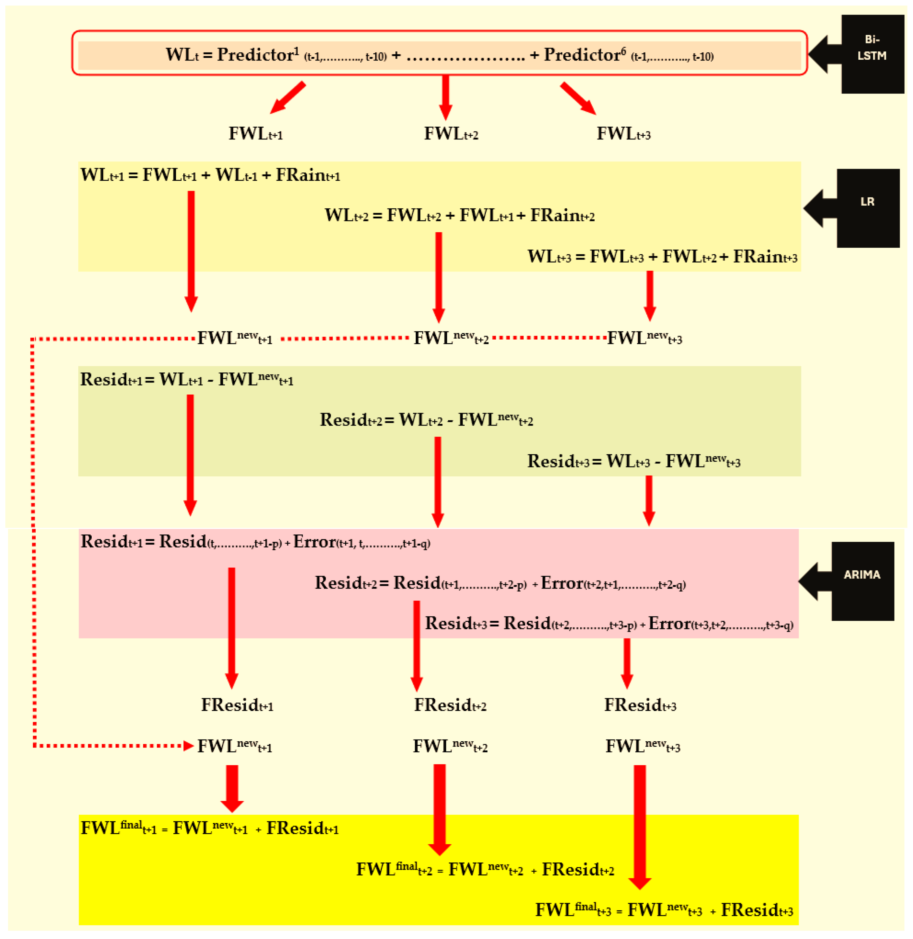
3.3. Improving the Accuracy of Forecasts Obtained by the Bi-LSTM Model

To further improve the forecasts obtained by the Vanilla Bi-LSTM model (i.e., Model A), these forecasts, together with the rainfall forecasts produced by our previous work [38], were incorporated into a base model to predict the actual WL. As mentioned in Section 1, this was because the water level of a river on a given day is expected to rise as a result of a considerable amount of rainfall on that same day.

Improvements were made to the forecasts obtained for the years 2017, 2018, and 2019, with the accumulating training periods starting from 2016. To integrate the actual WLs with both forecasted WLs and forecasted rainfall using a simple statistical model, a separate model using the Linear Regression approach (Model B) was introduced.

However certain assumptions needed be given thorough attention before applying the Regression modeling technique to the time series variables considered. One important aspect is the dependency between the time series observations. This was addressed by estimating regression parameters with the GLS estimation method.

When improving 1-day-ahead WL forecasts, the actual WL was modeled on the 1-day-ahead WL forecast, the actual water level at the previous day, and the 1-day-ahead rainfall forecast. The 2-day-ahead forecast was improved in the same way, but the actual water level on the previous day was replaced with the 1-day-ahead WL forecast since the actual WL for the second day would not be available at the time of forecasting. Likewise, the 3-day-ahead WL forecast was improved by modeling the 3-day-ahead actual WL on 3-day-ahead WL forecast, the 2-day-ahead WL forecast, and 3-day-ahead rainfall forecast.

This model was initially tested on the data for the year 2017. Since this integrated approach produced improved forecasts, we proceeded with Model B to generate improved forecasts for the rest of the years, 2018 and 2019.

Table 7. The performance of the improved Model B for the years 2017, 2018, and 2019.

Year	Forecasting Horizon	Actual	Forecasted					Total
			No	Alert	Minor	Major	Critical
2017	p1	No Flood	343	5				348
		Alert		10	2			12
		Minor					1	1
		Major						0
		Critical					2	2
	p2	No Flood	344	4				348
		Alert		9	3			12
		Minor				1		1
		Major						0
		Critical					2	2
	p3	No Flood	342	6				348
		Alert	1	6	5			12
		Minor			1			1
		Major						0
		Critical					2	2
2018	Forecasting Horizon	Actual	Forecasted					Total
			No	Alert	Minor	Major	Critical
	p1	No Flood	351	2				353
		Alert		6	1			7
		Minor			2			2
		Major						0
		Critical						0
	p2	No Flood	351	2				353
		Alert	1	4	2			7
		Minor			2			2
		Major						0
		Critical						0
	p3	No Flood	350	3				353
		Alert	2	3	2			7
		Minor			2			2
		Major						0
		Critical						0
2019	Forecasting Horizon	Actual	Forecasted					Total
			No	Alert	Minor	Major	Critical
	p1	No Flood	353	4				357
		Alert	1	3	1			5
		Minor						0
		Major						0
		Critical						0
	p2	No Flood	354	3				357
		Alert	3	1	1			5
		Minor						0
		Major						0
		Critical						0
	p3	No Flood	352	5				357
		Alert	3	2				5
		Minor						0
		Major						0
		Critical						0

compares the performances of the fitted models by separating the WLs into the flood risk levels as set out in Section 3.2. Overall, Model B shows an improved performance in terms of the forecasting accuracy for the longest forecasting period considered (i.e., 3 days ahead) and also the severity of the flood level.

In 2018, only ‘Alert’ and ‘Minor’ level flood events occurred. It is remarkable that all the ‘Minor’ flood events were forecasted accurately by Model B, a result which could not be attained by Model A (Vanilla Bi-LSTM), as shown in Table 5a. Similarly, the high forecasting ability of Model B can be noticed in 2017. It forecasts ‘Critical’ events accurately in each time-step. Furthermore, the capability of the improved model (Model B) in forecasting ‘Alert Levels’ of floods is satisfactory. An accurate forecasting of the only ‘Minor’ flood event happened in 2017 was misidentified by the improved model in its 1st two days ahead forecasts. However, those events were identified as risk levels even though mis-classified as high-risk flood events (i.e., ‘Critical’ or ‘Major’).

Table 8. The forecasting accuracy of Model B for the testing periods of 2017, 2018, and 2019.

Year	Forecasting Accuracy
	p1	p2	p3
2017	96%	94%	89%
2018	92%	87%	81%
2019	92%	83%	69%

summarizes the forecasting accuracy of Model B for test periods from 2017 to 2019. A summary of the results obtained by Model B for this entire period is depicted in Spreadsheets S5.

According to the table, it can be noticed that the fitted model (i.e., Model B) could produce improved forecasts for WLs, with more than 65% accuracy, though the accuracy decreases as the forecasting horizon increases.

3.4. Further Investigating the Validity of the Models: Model Performance with Recent Data

The validity of the aforementioned hybrid approach (Model B) was further tested using recently available data (i.e., from 2020) with the same set of predictor variables. The previously trained Vanilla Bi-LSTM model for 2014–2018 was used to forecast the WLs in 2020. Then, the fitted Regression model for the period 2016–2018 was used to improve WL forecasts for 2020. Another reason for continuing the validation process was to assess the adequacy of the finally fitted model in generating better forecasts for the extended period without re-training.

Within the period considered, only four events with an ‘Alert Level’ of flood risk appeared.

Table 9. The performance of Model A and Model B for the year 2020.

Year	Forecasting Horizon	Actual	Forecasted					Total
			No	Alert	Minor	Major	Critical
2020 Model A	p1	No Flood	360					360
		Alert		4				4
		Minor						0
		Major						0
		Critical						0
	p2	No Flood	360					360
		Alert		4				4
		Minor						0
		Major						0
		Critical						0
	p3	No Flood	360					360
		Alert	1	3				4
		Minor						0
		Major						0
		Critical						0
2020 Model B	Forecasting Horizon	Actual	Forecasted					Total
			No	Alert	Minor	Major	Critical
	p1	No Flood	358	2				360
		Alert		3	1			4
		Minor						0
		Major						0
		Critical						0
	p2	No Flood	358	2				360
		Alert		4				4
		Minor						0
		Major						0
		Critical						0
	p3	No Flood	355	5				360
		Alert		2	2			4
		Minor						0
		Major						0
		Critical						0

and

Table 10. Forecasting accuracy of Regression model for 2020.

Year	Forecasting Accuracy
	p1	p2	p3
2020	94%	86%	72%

demonstrate the performance of the Vanilla Bi-LSTM model (Model A) and the improved model (Model B). The models’ summaries can be found in Spreadsheets S5.

The comparison of these model performances implies that the hybrid model that uses both Bi-LSTM and Multiple Linear Regression did not forecast the ‘Alert Level’ flood events as ‘No Flood’ events for any forecasting horizon, even though it recognized some of those events as ‘Minor’ flood events. However, Table 9 evidences the weak performance of Model B. The comparison of these model performances implies that the Vanilla Bi-LSTM model (Model A) is more suitable for forecasting lower flood levels, whereas when the focus is to forecast critical flood levels with a longer forecasting horizon, the hybrid model that uses both Bi-LSTM and Linear Regression (i.e., Model B) is more appropriate.

The forecasting accuracy for each time-step depicts the same performance pattern shown in the previous section. Even though it decreases slightly when the forecast horizon increases, the percentage is always above 70%.

3.5. Residual Analysis of Model B and Modeling to Reduce Forecasting Error

As Model B produced three Time Series Regression models (corresponding to the three forecasting horizons considered), the residuals of these models were thoroughly examined. First, the stationarity of the three residual series were tested using the ADF test. Then, ACF and PACF plots were obtained to check for significant autocorrelation and partial autocorrelations. If the plots showed significant spikes at initial lags, a suitable ARIMA model was built for the residual series. Again, the residuals of the ARIMA models were examined to confirm if they followed the White Noise series using the Ljung–Box test. The summary of the fitted models is depicted in

Table 11. Summary of residual analysis and ARIMA models fitted for 2017–2019 and 2020.

Year	Forecasting Horizon	p1	p2	p3
2017	Stationarity of residuals of Model B	Stationary	Stationary	Stationary
	Fitted ARIMA model	ARIMA(2,0,3)	ARIMA(1,0,1)	ARIMA(2,0,1)
	Whether residuals of ARIMA model follow WN	Yes	Yes	Yes
2018	Stationarity of residuals of Model B	Stationary	Stationary	Stationary
	Fitted ARIMA model	ARIMA(2,0,3)	ARIMA(1,0,1)	ARIMA(1,0,1)
	Whether residuals of ARIMA model follow WN	Yes	Yes	Yes
2019	Stationarity of residuals of Model B	Stationary	Stationary	Stationary
	Fitted ARIMA model	ARIMA(2,0,2)	No significant autocorrelation	ARIMA(2,0,1)
	Whether residuals of ARIMA model follow WN	Yes	Yes	Yes
2020	Stationarity of residuals of Model B	Stationary	Stationary	Stationary
	Fitted ARIMA model	ARIMA(2,0,2)	ARIMA(1,0,1)	ARIMA(3,0,1)
	Whether residuals of ARIMA model follow WN	Yes	Yes	Yes

. A complete illustration of the residual analysis including ACF and PACF plots for the entire study period is shown in Spreadsheets S5.

Forecasts for the months that showed high WL rises (these events mostly appeared in the month of May) were obtained using the fitted ARIMA models. The final WL forecasts were obtained by adding those forecasted values obtained from the ARIMA models to the WL forecasts obtained from the improved Model B. The results are illustrated in Spreadsheets S5. Even though the final WL forecasts slightly improved upon the forecasts obtained from the hybrid model, there was not much of an effect on flood risk categorization, especially on the high flood risk levels. However, the misclassification of the two ‘Alert Level’ events in the 3-day-ahead forecast mentioned in Section 3.4 was slightly improved after adjustments to the residual series. One ‘Alert Level’ event was forecasted with a value of 19.51 m MSL (very close to the upper bound of ‘Alert Level’, 19.5 m MSL) by the final model and was forecasted as 19.77 m MSL by Model B. Overall, this implies that the results generated by the hybrid model are good enough for issuing accurate flood warnings.

Moreover, the results indicate the superiority of the hybrid model which combines Vanilla Bi-LSTM and a Time Series Regression model with the GLS estimation method. This model is capable of producing accurate forecasts of WLs, thereby predicting the flood risk level at the target station. This was an unachievable target for many past studies. Obtaining flood risk levels based on WL forecasts produces more precise warnings since direct flood risk forecasting leads to an imbalance classification problem. The severe imbalance in flood levels imposes an additional challenge for researchers, who must select effective resampling methods to achieve data balance. By overcoming these aforementioned challenges, the hybrid model proposed in this study is capable of forecasting even severe flood events 3 days in advance. Moreover, this augmented flood forecasting approach enables a significant lead time for better flood preparedness. Therefore, the proposed methodology suits the forecasting of flood events for the highly vulnerable Ratnapura area.

4. Conclusions

This study proposes a novel hybrid forecasting approach which combines deep learning with a traditional statistical method, Time Series Regression. The study also applies two statistical techniques (the Granger Causality test and cross-correlation analysis) for feature selection to model WLs at Ratnapura. The novelty of the study lies in its sequential modeling of WLs at the target station with Bi-LSTM and its improving of forecasting accuracy, especially of the actionable levels of floods (Minor to Critical) by incorporating the Time Series Regression model. Further, this model is capable of capturing the real-time weather dynamics created by the unexpected occurrence of a rainfall event. Therefore, this dynamic hybrid model shows better performance than that of the Vanilla Bi-LSTM model in terms of forecasting accuracy.

The current study enables a significant forecasting horizon of 3 days, providing a considerable time gap for taking flood mitigatory measures that could not be attained by past studies [9,33,34] performed based on different river basins in Sri Lanka. Moreover, our study has carried out several trials of validation to verify the applicability and accuracy of the hybrid model, which was given meager concern by previous work (e.g., [32]). The study [24] that used a Neurofuzzy model for short-term flood forecasting in the Kolar Basin in India could only capture 47.95% of the peak flow values that caused flood events. This rate of accuracy was enabled only in its one-hour-ahead forecast. The hybrid model introduced in our study is capable of forecasting flood events with more than 80% accuracy in its one- and two-days-ahead forecasts, while producing accuracy of 65% in its three-days-ahead forecast. Moreover, the proposed model performs well in forecasting actionable flood events, with an accuracy of 80% or more across all forecasting horizons.

The unavailability of some important predictors such as soil moisture and river velocity, the significant percentage of missingness among WL data, and the lack of superior computer power in training the models are identified as major limitations of this study. The fitted model in this study uses data from only a few nearby WL gauging stations that are currently in function. A better performance could have been achieved if data from a higher number of nearby WL gauging stations were available.

Going further ahead, our future work aims to obtain the spreads of inundation (as maps) based on river discharge data and forecasted WLs. This will facilitate the clear presentation of flood risk assessments and the issuance of warnings to civilians settled down in the down-stream area of the river basin in advance of a devastating outcome. The overall methodology has potential to be developed as an accurate flood forecasting and warning system, for which there is still a high demand in Sri Lanka and also at the global level. Furthermore, the proposed hybrid model can be tested on WL data of other flood-susceptible river basins in Sri Lanka. Additionally, the modeling approach proposed in this study could be applied, with suitable adjustments, to generate flood warning systems around the globe.

References

1. Palash, W.; Akanda, A.S.; Islam, S. A data-driven global flood forecasting system for medium to large rivers. Sci. Rep. 2024, 14, 8979. [Google Scholar] [CrossRef]
2. Chapter 8—Floodplain Definition and Flood Hazard Assessment. Available online: https://www.oas.org/osde/publications/Unit/oea66e/ch08.htm#:~:text=Floodplains%20are%2C%20in%20general%2C%20those,activities%20exceeds%20an%20acceptable%20level (accessed on 20 December 2024).
3. Ekwueme, B.N. Machine learning based prediction of urban flood susceptibility from selected rivers in a tropical catchment area. Civ. Eng. J. 2022, 8, 1857. [Google Scholar] [CrossRef]
4. Jain, S.K.; Mani, P.; Jain, S.K.; Prakash, P.; Singh, V.P.; Tullos, D.; Kumar, S.; Agarwal, S.P.; Dimri, A.P. A Brief review of flood forecasting techniques and their applications. Int. J. River Basin Manag. 2018, 16, 329–344. [Google Scholar] [CrossRef]
5. Adams, T.E.; Gangodagamage, C.; Pagano, T.C. (Eds.) Flood Forecasting: A Global Perspective; Elsevier: Amsterdam, The Netherlands, 2024. [Google Scholar]
6. Karyotis, C.; Maniak, T.; Doctor, F.; Iqbal, R.; Palade, V.; Tang, R. Deep learning for flood forecasting and monitoring in urban environments. In Proceedings of the 2019 18th IEEE International Conference on Machine Learning and Applications (ICMLA), Boca Raton, FL, USA, 16–19 December 2019; IEEE: Piscataway, NJ, USA, 2019; pp. 1392–1397. [Google Scholar]
7. Nevo, S.; Morin, E.; Gerzi Rosenthal, A.; Metzger, A.; Barshai, C.; Weitzner, D.; Voloshin, D.; Kratzert, F.; Elidan, G.; Dror, G.; et al. Flood forecasting with machine learning models in an operational framework. Hydrol. Earth Syst. Sci. 2022, 26, 4013–4032. [Google Scholar] [CrossRef]
8. Prieto, C.; Patel, D.; Han, D.; Dewals, B.; Bray, M.; Molinari, D. Preface: Advances in pluvial and fluvial flood forecasting and assessment and flood risk management. Nat. Hazards Earth Syst. Sci. 2024, 24, 3381–3386. [Google Scholar] [CrossRef]
9. Nandalal, K.D.W. Use of a hydrodynamic model to forecast floods of Kalu River in Sri Lanka. J. Flood Risk Manag. 2009, 2, 151–158. [Google Scholar] [CrossRef]
10. Shao, Y.; Chen, J.; Zhang, T.; Yu, T.; Chu, S. Advancing rapid urban flood prediction: A spatiotemporal deep learning approach with uneven rainfall and attention mechanism. J. Hydroinform. 2024, 26, 1409–1424. [Google Scholar] [CrossRef]
11. Byaruhanga, N.; Kibirige, D.; Gokool, S.; Mkhonta, G. Evolution of Flood Prediction and Forecasting Models for Flood Early Warning Systems: A Scoping Review. Water 2024, 16, 1763. [Google Scholar] [CrossRef]
12. Sit, M.; Demir, I. Decentralized flood forecasting using deep neural networks. arXiv 2019, arXiv:1902.02308. [Google Scholar]
13. Mishra, S.; Dwivedi, V.K.; Sarvanan, C.; Pathak, K.K. Pattern discovery in hydrological time series data mining during the monsoon period of the high flood years in Brahmaputra river basin. Int. J. Comput. Appl. 2013, 67, 7–14. [Google Scholar] [CrossRef]
14. Wang, D.; Ding, W.; Yu, K.; Wu, X.; Chen, P.; Small, D.L.; Islam, S. Towards long-lead forecasting of extreme flood events: A data mining framework for precipitation cluster precursors identification. In Proceedings of the 19th ACM SIGKDD International Conference on Knowledge Discovery and Data Mining, Chicago, IL, USA, 11–14 August 2013; pp. 1285–1293. [Google Scholar]
15. Damle, C. Flood Forecasting Using Time Series Data Mining. Master’s Thesis, University of South Florida, Tampa, FL, USA, 2005. [Google Scholar]
16. Pradhan, B.; Youssef, A.M. A 100-year maximum flood susceptibility mapping using integrated hydrological and hydrodynamic models: Kelantan River Corridor, Malaysia. J. Flood Risk Manag. 2011, 4, 189–202. [Google Scholar] [CrossRef]
17. Xu, Q.; Shi, Y.; Bamber, J.L.; Ouyang, C.; Zhu, X.X. Large-scale flood modeling and forecasting with FloodCast. Water Res. 2024, 264, 122162. [Google Scholar] [CrossRef]
18. Liong ShieYui, L.S.; Sivapragasam, C. Flood stage forecasting with support vector machines. JAWRA J. Am. Water Resour. Assoc. 2002, 38, 173–186. [Google Scholar] [CrossRef]
19. Hayder, I.M.; Al-Amiedy, T.A.; Ghaban, W.; Saeed, F.; Nasser, M.; Al-Ali, G.A.; Younis, H.A. An intelligent early flood forecasting and prediction leveraging machine and deep learning algorithms with advanced alert system. Processes 2023, 11, 481. [Google Scholar] [CrossRef]
20. Dtissibe, F.Y.; Ari, A.A.A.; Abboubakar, H.; Njoya, A.N.; Mohamadou, A.; Thiare, O. A comparative study of Machine Learning and Deep Learning methods for flood forecasting in the Far-North region, Cameroon. Sci. Afr. 2024, 23, e02053. [Google Scholar] [CrossRef]
21. Campolo, M.; Andreussi, P.; Soldati, A. River flood forecasting with a neural network model. Water Resour. Res. 1999, 35, 1191–1197. [Google Scholar] [CrossRef]
22. Zhang, B.; Ouyang, C.; Cui, P.; Xu, Q.; Wang, D.; Zhang, F.; Li, Z.; Fan, L.; Lovati, M.; Liu, Y.; et al. Deep learning for cross-region streamflow and flood forecasting at a global scale. Innovation 2024, 5, 100617. [Google Scholar] [CrossRef]
23. Yu, P.S.; Chen, S.T.; Chang, I.F. Support vector regression for real-time flood stage forecasting. J. Hydrol. 2006, 328, 704–716. [Google Scholar] [CrossRef]
24. Nayak, P.C.; Sudheer, K.P.; Rangan, D.M.; Ramasastri, K.S. Short-term flood forecasting with a neurofuzzy model. Water Resour. Res. 2005, 41, W04004. [Google Scholar] [CrossRef]
25. Balogun, A.L.; Adebisi, N. Sea level prediction using ARIMA, SVR and LSTM neural network: Assessing the impact of ensemble Ocean-Atmospheric processes on models’ accuracy. Geomat. Nat. Hazards Risk 2021, 12, 653–674. [Google Scholar] [CrossRef]
26. Damavandi, H.G.; Shah, R.; Stampoulis, D.; Wei, Y.; Boscovic, D.; Sabo, J. Accurate prediction of streamflow using long short-term memory network: A case study in the Brazos River Basin in Texas. Int. J. Environ. Sci. Dev. 2019, 10, 294–300. [Google Scholar] [CrossRef]
27. Smyl, S. A hybrid method of exponential smoothing and recurrent neural networks for time series forecasting. Int. J. Forecast. 2020, 36, 75–85. [Google Scholar] [CrossRef]
28. Al-Amiedy, T.A.; Anbar, M.; Belaton, B.; Kabla, A.H.H.; Hasbullah, I.H.; Alashhab, Z.R. A systematic literature review on machine and deep learning approaches for detecting attacks in RPL-based 6LoWPAN of internet of things. Sensors 2022, 22, 3400. [Google Scholar] [CrossRef]
29. Hu, Y.; Yan, L.; Hang, T.; Feng, J. Stream-flow forecasting of small rivers based on LSTM. arXiv 2020, arXiv:2001.05681. [Google Scholar]
30. Xiang, Z.; Yan, J.; Demir, I. A rainfall-runoff model with LSTM-based sequence-to-sequence learning. Water Resour. Res. 2020, 56, e2019WR025326. [Google Scholar] [CrossRef]
31. Won, Y.M.; Lee, J.H.; Moon, H.T.; Moon, Y.I. Development and application of an urban flood forecasting and warning process to reduce urban flood damage: A case study of Dorim River basin, Seoul. Water 2022, 14, 187. [Google Scholar] [CrossRef]
32. Nandalal, H.K.; Ratnayake, U.R. Flood risk analysis using fuzzy models. J. Flood Risk Manag. 2011, 4, 128–139. [Google Scholar] [CrossRef]
33. Hettiarachchi, N.; Thilakumara, R.P. Water level forecasting and flood warning system: A Neuro-Fuzzy Approach. Int. J. Appl. Eng. Res 2014, 9, 4901–4904. [Google Scholar]
34. Ratnayake, U.; Sachindra, D.A.; Nandalal, K.D.W. Rainfall Forecasting for Flood Prediction in the Nilwala Basin. 2010. Available online: http://www.civil.mrt.ac.lk/web/conference/ICSBE_2010/vol_02/53.pdf (accessed on 1 January 2025).
35. Vinokić, L.; Dotlić, M.; Prodanović, V.; Kolaković, S.; Simonovic, S.P.; Stojković, M. Effectiveness of three machine learning models for prediction of daily streamflow and uncertainty assessment. Water Res. X 2025, 27, 100297. [Google Scholar] [CrossRef]
36. Kordani, M.; Nikoo, M.R.; Fooladi, M.; Ahmadianfar, I.; Nazari, R.; Gandomi, A.H. Improving long-term flood forecasting accuracy using ensemble deep learning models and an attention mechanism. J. Hydrol. Eng. 2024, 29, 04024042. [Google Scholar] [CrossRef]
37. Kumar, V.; Azamathulla, H.M.; Sharma, K.V.; Mehta, D.J.; Maharaj, K.T. The state of the art in deep learning applications, challenges, and future prospects: A comprehensive review of flood forecasting and management. Sustainability 2023, 15, 10543. [Google Scholar] [CrossRef]
38. Saubhagya, S.; Tilakaratne, C.; Lakraj, P.; Mammadov, M. Granger Causality-Based Forecasting Model for Rainfall at Ratnapura Area, Sri Lanka: A Deep Learning Approach. Forecasting 2024, 6, 1124–1151. [Google Scholar] [CrossRef]
39. Rasmy, M.; Yasukawa, M.; Ushiyama, T.; Tamakawa, K.; Aida, K.; Seenipellage, S.; Hemakanth, S.; Kitsuregawa, M.; Koike, T. Investigations of multi-platform data for developing an integrated flood information system in the Kalu River Basin, Sri Lanka. Water 2023, 15, 1199. [Google Scholar] [CrossRef]
40. Darkwah, G.K.; Kalyanapu, A.; Owusu, C. Machine Learning-Based Flood Forecasting System for Window Cliffs State Natural Area, Tennessee. GeoHazards 2024, 5, 64–90. [Google Scholar] [CrossRef]
41. Wang, Y.; Wang, W.; Zang, H.; Xu, D. Is the LSTM Model Better than RNN for Flood Forecasting Tasks? A Case Study of HuaYuankou Station and LouDe Station in the Lower Yellow River Basin. Water 2023, 15, 3928. [Google Scholar] [CrossRef]
42. Probst, W.N.; Stelzenmüller, V.; Fock, H.O. Using cross-correlations to assess the relationship between time-lagged pressure and state indicators: An exemplary analysis of North Sea fish population indicators. ICES J. Mar. Sci. 2012, 69, 670–681. [Google Scholar] [CrossRef]
43. RIVERNET.LK, Early Warning System. Available online: https://rivernet.lk/_landing/ (accessed on 1 January 2025).
44. Hettiarachchi, P. Inundation Maps of the Kalu Ganga Basin During the Flood in May 2003; Department of Irrigation: Colombo, Sri Lanka, 2013.
45. Chatfield, C.; Xing, H. The Analysis of Time Series: An Introduction with R; Chapman and hall/CRC: Boca Raton, FL, USA, 2019. [Google Scholar]
46. Overview for Cross Correlation. Available online: https://support.minitab.com/en-us/minitab/help-and-how-to/statistical-modeling/time-series/how-to/cross-correlation/before-you-start/overview/ (accessed on 1 January 2025).
47. Zhou, J.; Lu, Y.; Dai, H.N.; Wang, H.; Xiao, H. Sentiment analysis of Chinese microblog based on stacked bidirectional LSTM. IEEE Access 2019, 7, 38856–38866. [Google Scholar] [CrossRef]
48. James, G.; Witten, D.; Hastie, T.; Tibshirani, R. An Introduction to Statistical Learning; Springer: New York, NY, USA, 2013; Volume 112, p. 18. [Google Scholar]
49. Kariya, T.; Kurata, H. Generalized Least Squares; John Wiley & Sons: Hoboken, NJ, USA, 2004. [Google Scholar]
50. Saubhagya, S.; Tilakaratne, C.; Lakraj, P.; Mammadov, M. A Novel Hybrid Spatiotemporal Missing Value Imputation Approach for Rainfall Data: An Application to the Ratnapura Area, Sri Lanka. Appl. Sci. 2024, 14, 999. [Google Scholar] [CrossRef]
Figure 1. The WL gauging stations of the Kalu River Basin [44]. (The direction of water flow (in blue) is from right to left. The upper-stream WL gauging stations, Dela and Malwala, contain missing values for long periods. This made it difficult to build one model that incorporated both stations).
Forecasting 07 00029 g001
Figure 2. The time periods of data for each main stage of the study.
Forecasting 07 00029 g002
Figure 3. LSTM structure diagram.
Forecasting 07 00029 g003
Figure 4. Bi-LSTM models with moving windows for training and testing.
Forecasting 07 00029 g004
Figure 5. Vanilla Bi-LSTM model description for testing performance consistency.
Forecasting 07 00029 g005