Dynamic Forecasting of Gas Consumption in Selected European Countries

Abstract

Natural gas consumption in Europe has undergone substantial changes in recent years, driven by geopolitical tensions, economic dynamics, and the continent’s ongoing transition towards cleaner energy sources. Furthermore, as noted in the International Energy Agency’s Gas Market Report 2025, natural gas demand is becoming increasingly sensitive to fluctuations in weather patterns, including cold snaps and heatwaves. These factors make the task of forecasting future annual consumption particularly challenging from a statistical perspective and underscore the importance of accurately quantifying the uncertainty surrounding predictions. In this paper, we propose a simple yet flexible approach to issuing dynamic probabilistic forecasts based on an additive time series model. To capture long-term trends, the model incorporates a deterministic component based on the Guseo–Guidolin innovation diffusion framework. In addition, a stochastic innovation term governed by an ARIMAX process is used to describe year-over-year fluctuations, helping to account for the potential presence of variance nonstationarity over time. The proposed methodology is applied to forecast future annual consumption in six key European countries: Austria, France, Germany, Italy, the Netherlands, and the United Kingdom.

1. Introduction

Natural gas consumption in Europe has undergone significant changes in recent years, driven by geopolitical tensions, economic factors, and the continent’s transition toward cleaner energy. Traditionally reliant on imports from Russia, European countries have diversified their energy sources following the 2022 invasion of Ukraine, leading to a sharp decline in Russian pipeline gas and a surge in liquefied natural gas imports from the U.S., Qatar, and others. Total gas demand dropped in 2022 and 2023 due to high prices, energy conservation efforts, and a shift towards renewables (see, e.g., [1]). The decline was especially notable in industrial sectors, which reduced production or switched fuels. Despite this, natural gas remains an important part of Europe’s energy mix as the region gradually transitions to a more sustainable and energy-secure future, particularly for heating and backup power generation.

According to the International Energy Agency Gas Market Report 2025, natural gas demand is becoming more sensitive to changes in weather patterns, including cold snaps and heat waves. Climate change is driving more extreme weather events; at the same time gas-based generation plays an increasingly important backup role in markets with a growing share of variable renewables, where it ensures security of the electricity supply at times when wind and/or solar output is low.

In Europe, slow wind speeds in the first half of November 2024 led to a sharp decline in wind power output year-over-year. Gas-fired power plants played a key role in providing backup to the power system, seeing their output increase by nearly 80% year-over-year. Higher gas demand was primarily met through larger storage withdrawals. Even if it is still uncertain what caused the massive blackout in Spain and Portugal at the end of April 2025, it is hypothesized that a sudden decrease in renewable energy production could have unbalanced the electricity network, where natural gas would have ensured stability.

These events highlight the need for a careful assessment of investment in the assets that enable the secure delivery of gas, including gas storage, as well as the development of mechanisms that allow for greater supply flexibility. In order to inform effective industrial planning and investments, it becomes critically important from a statistical perspective to forecast annual consumption levels for the coming years, with particular attention to quantifying the degree of uncertainty associated with the predictions and accounting for potential developments in key climatic factors such as temperature trends. Similar considerations have been suggested in [2], Section 1.1 as well as in [3].

The scientific literature on forecasting natural gas consumption has expanded recently as natural gas becomes an increasingly critical part of the global energy transition as well as for reasons concerning market volatility and environmental sustainability. Forecasting methodologies have evolved significantly over the past several decades, ranging from statistical models to machine learning and deep learning techniques, as highlighted in [4], for example. As outlined in [5], the development of forecasting models can be categorized into four stages. Time series models have proven to be the best models for long-term predictions, while artificial intelligence approaches show better results in short- and medium-term forecasting. Recent studies have emphasized the importance of incorporating external variables such as meteorological conditions [3] along with economic indicators such as GDP and inflation [6]. When focusing on short-term time horizons, recent approaches based on convolutional network models have been proposed to capture complex seasonal demand patterns by applying multiple seasonal-trend decompositions in order to separate time series into their periodic patterns and residual components; see, e.g., [7]. On a regional level, hybrid models have been proposed to address nonlinear trends, particularly in the European Union’s short-term monthly demand forecasts [8]. On the other hand, comprehensive reviews and scenario-based forecasting frameworks highlight the growing necessity of integrating environmental and sustainability factors into long-term demand modeling; see [9,10]. In particular, [10] observed that most long-term gas prediction studies fail to adequately consider environmental aspects; the authors stressed the importance of considering these influencing factors when forecasting gas demand from national and global perspectives.

The evolving landscape of natural gas demand reflects the need for new approaches that can inform strategic energy planning and policy-making in an era of rapid change. Embracing this perspective, we take a long-term perspective in this paper by modeling the annual consumption of natural gas in a selected number of European countries while accounting for the possible effect exerted by the change in temperatures. In particular, our modeling approach builds upon a well-accepted methodology to capture nonlinear trends in annual energy consumption data, then proposes a subsequent forecasting procedure for proper management of the residual variability observed in the data.

The most comprehensive and suitable form of forecasting in this context is probabilistic, relying on the construction of entire predictive distributions for the quantities of interest; see, e.g., [11,12,13]. However, this approach presents several challenges due to the dynamic structure of the forecasting task within a time-dependent framework and the limited availability of data, which renders non- and semi-parametric methods impractical; see, e.g., [14], Ch. 12.7.

Therefore, an effective solution for probabilistic forecasting of annual consumption levels requires models with a moderate number of parameters as well as sufficient flexibility to account for the variability in temperature patterns and accurately capture the evolving dynamics of gas consumption. In this work, we propose a dynamic forecasting method based on an additive time series model that addresses such desiderata. The latter incorporates a deterministic component based on the Guseo–Guidolin model (GGM) [15] to capture long-term trends alongside a stochastic innovation term governed by an autoregressive integrated moving average process with explanatory variables (ARIMAX) to describe annual fluctuations. This approach accounts for both mean drifts and potential variance nonstationarity over time of gas consumption levels. In particular, including mean surface air temperature (yearly average) as a covariate allows us to track consumption variations spurred by fluctuations in climate conditions.

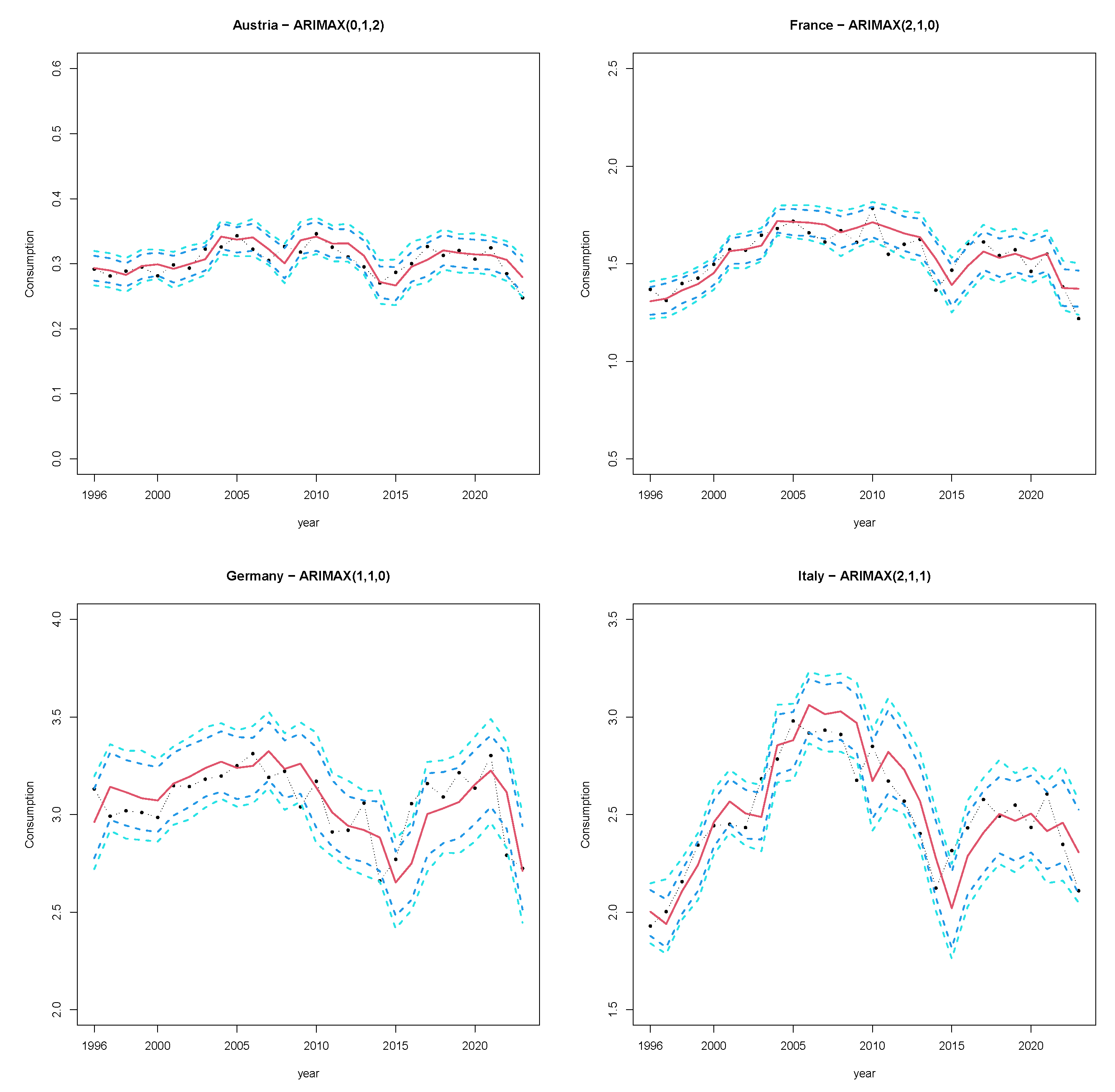
Methodologically, our procedure consists of two steps: first, the parameters of the GGM are estimated using the original series of consumption levels and the resulting trend estimate is used to filter the series; second, an ARIMAX model is fitted to the residual component using a Bayesian approach, which is well-suited for estimating the distribution of the (unobservable) innovations through the posterior predictive distribution. Afterwards, a predictive distribution for k-years-ahead gas consumption levels is obtained by shifting this estimate using the GGM projected trend. The proposed methodology is applied to forecast future consumption in six key European countries: Austria, France, Germany, Italy, the Netherlands, and the United Kingdom. We emphasize that our focus is on developing a procedure that reliably captures historical consumption trends across different countries and on using prediction intervals to offer plausible and dependable ranges for future gas consumption.

The rest of this paper is outlined as follows: in Section 2, we describe the gas consumption data and covariates used to train the forecasting methods across countries; in Section 3, we discuss the considered statistical models and predictive tools; in Section 4, we present the results of our analysis, which forecasts a reduction in gas consumption levels in the coming years up to 2028; finally, Section 5 briefly discusses possible directions for future work.

2. Data

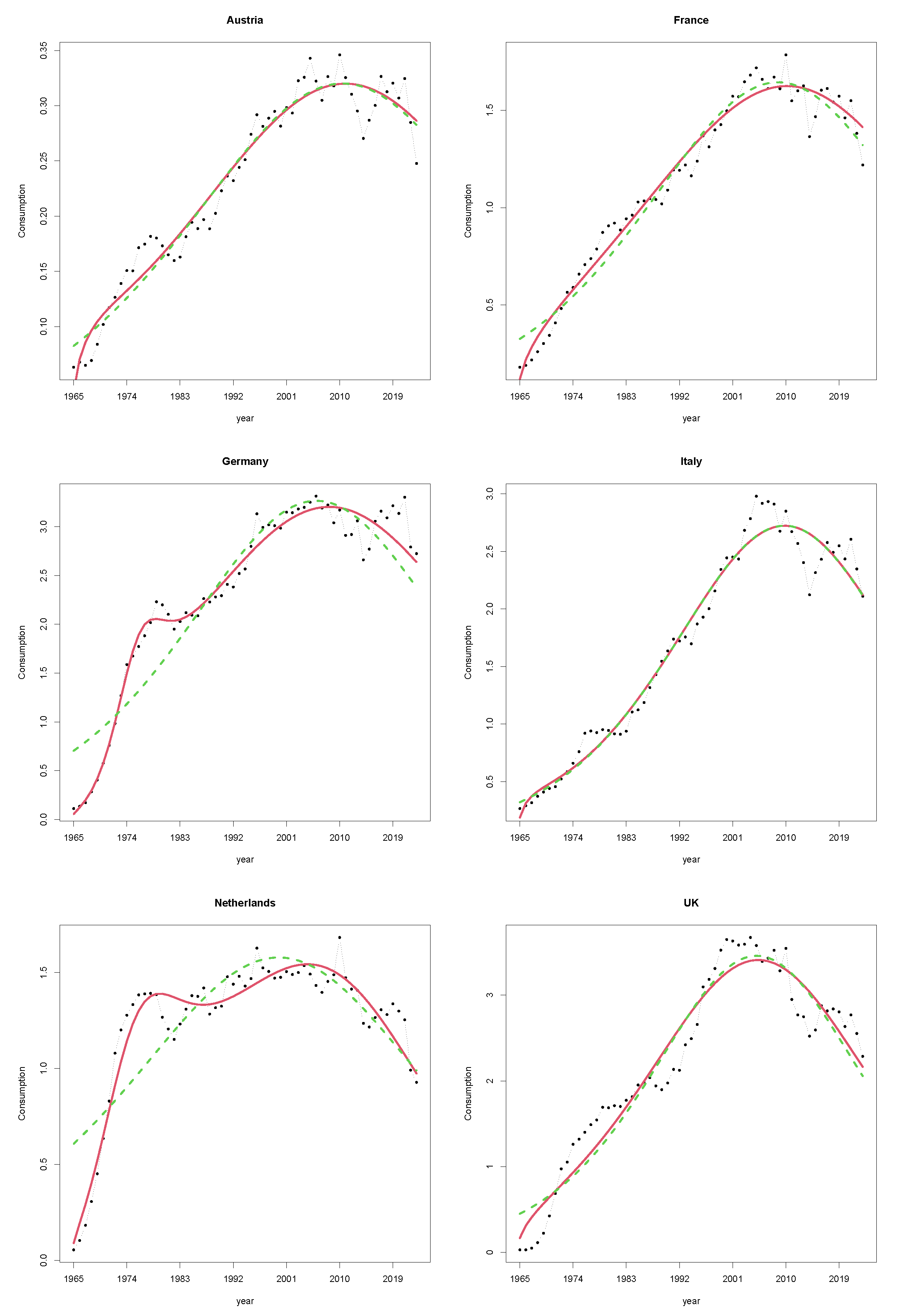
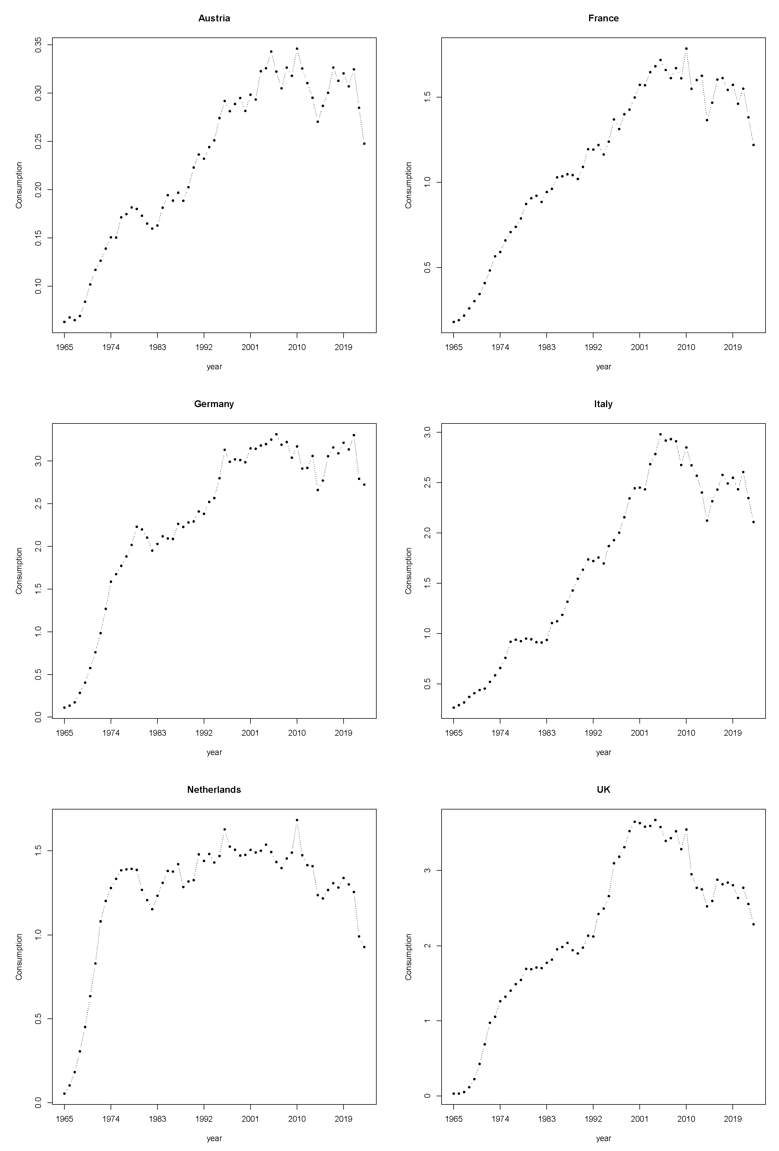
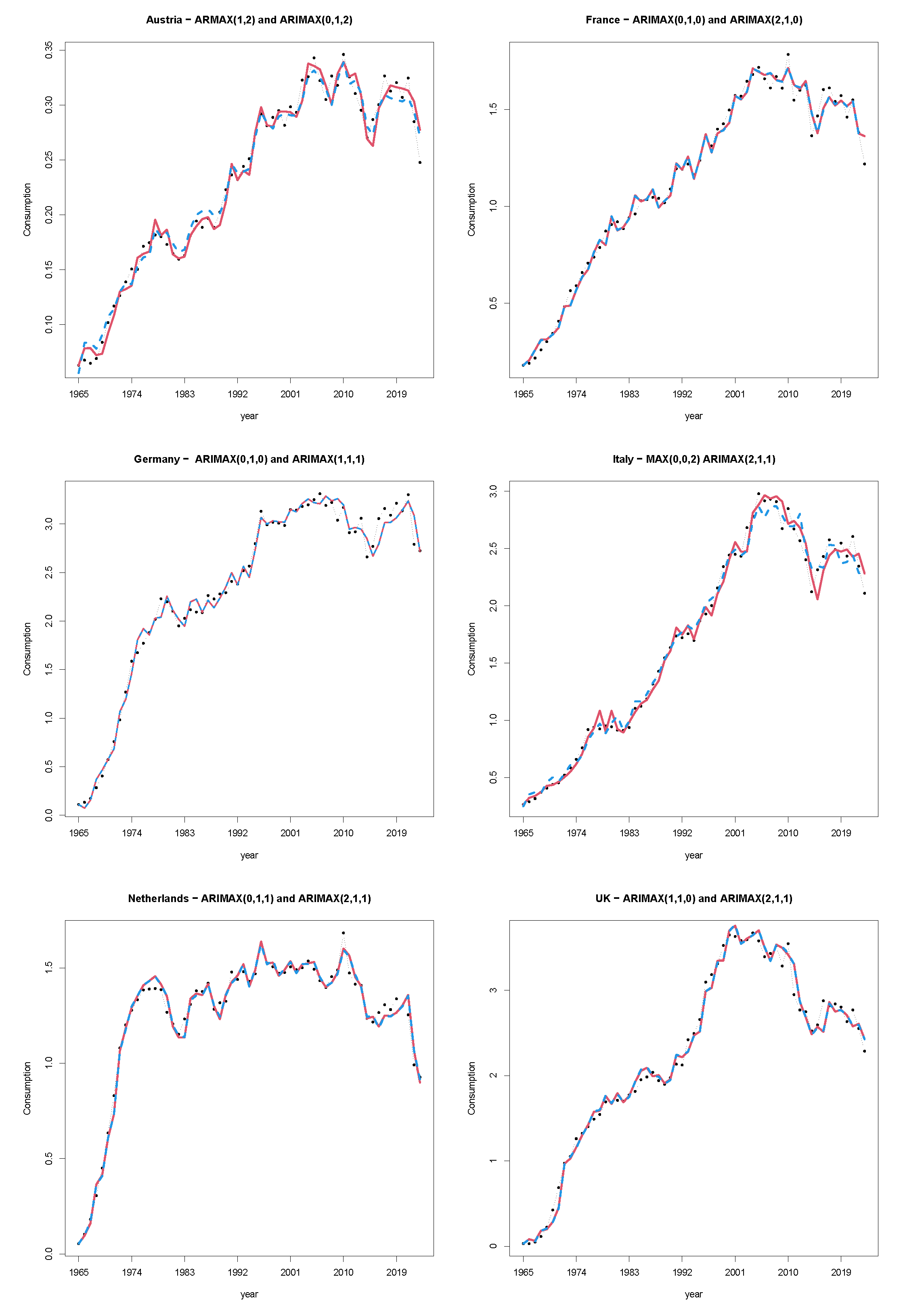
Our statistical analysis aims to predict gas consumption while accounting for temperature, which is known to significantly influence gas demand (e.g., [16]). Data on gas consumption from 1965 to 2023 were taken from the Energy Institute (see https://www.energyinst.org/statistical-review, accessed on 18 May 2025) on a yearly time interval. The consumption amounts exclude natural gas converted to liquid fuels but include derivatives of coal and natural gas consumed during gas-to-liquid transformation. Consumption in exajoules for Austria, France, Germany, Italy, and the UK from 1965 to 2023 is plotted in Figure 1. These countries were selected due to their being the largest consumers of natural gas in Europe (France, Germany, Italy, Netherlands, UK) in order to provide a general overview of the European landscape in terms of gas consumption. In contrast, Austria was selected as an example of a small country in order to test our model’s applicability to less central market contexts.

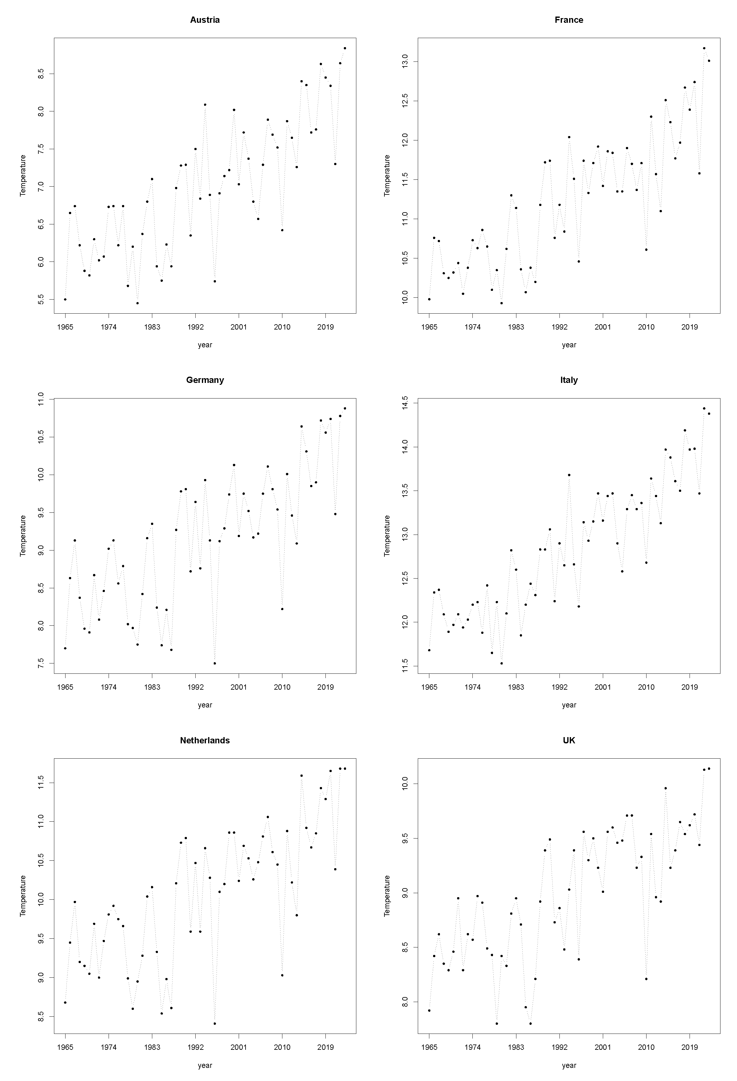
Following a sustained upward trend, a downward shift emerges across all six of these countries in the second decade of the 2000s. In particular, a strong year-over-year decline is visible in all countries in 2022, when natural gas demand in the European Union fell by 13.2%. This decline was concurrent with an increase in variability, making the prediction of consumption particularly difficult. We consider the observed annual average mean surface air temperature in centigrade degrees an explanatory variable. These data are publicly available from the World Bank through the Climate Change Knowledge Portal (see https://www.worldbank.org/en/topic/climatechange, accessed on 18 May 2025) and are reported in Figure 2 for the time window ranging from 1965 to 2023. With rising temperatures, all six countries are deemed vulnerable to climate change; in particular, an increasing risk of heat waves is reported for France and Germany, while an upward trend in extreme temperatures is recorded for Italy. As temperatures rise due to climate change, natural gas usage for heating is anticipated to decline. At the same time, electricity consumption for cooling is projected to increase, as recently highlighted for other geographic areas, e.g., by [17]. The ultimate goal of this work is to formalize this uptake in rigorous statistical terms using predictive distributions and prediction intervals.

3. Methods

This section illustrates the adopted statistical models and predictive inference techniques. We model gas consumption at time t in an additive fashion:

$$G_t=g(t;\vartheta )+Y_t$$

(1)

where $g(·;\vartheta )$ is a deterministic function of time depending on unknown parameters $\vartheta$ and where $\left(Y_t\right)$ is a stochastic non-observable time series. In particular, $g(·;\vartheta )$ describes the long-run trend of gas consumption, while the time series $\left(Y_t\right)$ captures the annual fluctuations around the trend, accounting for possible short-range dependence across years. In practice, our statistical methodology is based on preliminary estimation of parameters $\vartheta$ based on a finite stretch ${\left(G_t\right)}_{t=T_0}^T$ of gas consumption of length $n=T-T_0+1$. From this, we obtain fitted values of gas consumption ${\widehat{G}}_t^{\left(n\right)}=g(t;{\widehat{\vartheta }}_n)$, from which residuals $Y_t^{\left(n\right)}=G_t-{\widehat{G}}_t^{\left(T\right)}$ are then obtained. As illustrated in the next subsections, we model $g(t;\vartheta )$ through a diffusion equation, notably via GGM, and analyze residuals through ARIMAX time series models. By combining these two steps, k-steps-ahead point forecasts and predictive regions for future gas consumption can be produced.

3.1. GGM

Innovation diffusion models have been proven to be especially suitable in modeling the consumption dynamics of both nonrenewable and renewable energy sources. The literature on innovation diffusion models applied in the energy context expanded in the 2000s due to these models’ ability to effectively capture the nonlinear and evolutionary nature of energy consumption processes. Building on seminal works by [18,19], which suggested that innovation dynamics in energy systems are similar to those in other commercial sectors because new forms of energy need to be integrated into society, a growing body of contributions has studied the spread of energy technologies. This approach considers new energy technologies as new products that need to gain market acceptance through collective decisions and market mechanisms such as incentives, tariffs, and price changes, which are well captured by models such as the Bass model [20] and its extensions. A recent line of research has focused on the dominant role of nonrenewable energy technologies in the energy transition, leading to the development of multivariate models such as those employed in the works of [21,22,23]. For recent reviews on the use of innovation diffusion models in energy markets, see, e.g., [24,25,26].

The Guseo–Guidolin model (GGM) [15] was developed to provide a flexible extension to the basic Bass model that ensures greater predictive ability.

Following [15,25], this generalization of the BM considers a dynamic market potential $m\left(t\right)$, which can be formulated as

$$z^{\prime }\left(t\right)=m\left(t\right)\left[p+q{\displaystyle \frac{z\left(t\right)}{m\left(t\right)}}\right]\left[1-{\displaystyle \frac{z\left(t\right)}{m\left(t\right)}}\right]+m^{\prime }\left(t\right){\displaystyle \frac{z\left(t\right)}{m\left(t\right)}},t>0.$$

(2)

Equation (2) describes instantaneous adoptions $z^{\prime }\left(t\right)$ using a BM with $m\left(t\right)$ plus a factor $m^{\prime }\left(t\right)z\left(t\right)/m\left(t\right)$ that assigns $z^{\prime }\left(t\right)$ a portion of the variation of the market potential $m^{\prime }\left(t\right)$, which is the growth rate $z\left(t\right)/m\left(t\right)$. In Equation (2), the variation of the market potential $m^{\prime }\left(t\right)$ has an effect on instantaneous adoptions $z^{\prime }\left(t\right)$, which may be either positive and reinforcing (if $m\left(t\right)$ is increasing) or negative (if $m\left(t\right)$ is decreasing). This expresses the idea that a product’s adoption gains an extra benefit from an expanding market potential, whereas a declining market weakens the process. Equation (2) can be conveniently re-arranged as follows:

$${\displaystyle \frac{z^{\prime }\left(t\right)m\left(t\right)-z\left(t\right)m^{\prime }\left(t\right)}{m^2\left(t\right)}}={\left[{\displaystyle \frac{z\left(t\right)}{m\left(t\right)}}\right]}^{\prime }=\left[p+q{\displaystyle \frac{z\left(t\right)}{m\left(t\right)}}\right]\left[1-{\displaystyle \frac{z\left(t\right)}{m\left(t\right)}}\right].$$

(3)

Equation (3) provides a useful representation, which by setting $y\left(t\right)=z\left(t\right)/m\left(t\right)$ yields

$$y^{\prime }\left(t\right)=p+qy\left(t\right)(1-y\left(t\right)),$$

that is, the standard BM. The generalization of the BM, where $m\left(t\right)$ is time-dependent, has following closed-form solution:

$$z\left(t\right)=m\left(t\right){\displaystyle \frac{1-e^{-(p+q)t}}{1+\frac{q}{p}{e}^{-(p+q)t}}}.$$

(4)

Equation (4) clearly shows that $m\left(t\right)$ is a free function which multiplies the dynamics of the diffusion process expressed by parameters p and q. The function $m\left(t\right)$ may take several structures depending on the hypotheses about the market potential development.

In [15], a suitable specification for $m\left(t\right)$ was proposed by adopting the hypothesis that the development of the market potential depends on a communication process about the new product or technology, which typically precedes the adoption phase and serves the purpose of building the market.

In particular, the dynamic market potential $m\left(t\right)$ is defined according to a BM-like structure:

$$m\left(t\right)=K\sqrt{{\displaystyle \frac{1-e^{-(p_c+q_c)t}}{1+\frac{q_c}{p_c}{e}^{-(p_c+q_c)t}}}}.$$

(5)

In Equation (5), the parameters $p_c$ and $q_c$ govern the communication process. The parameter $p_c$ describes the behavior of innovative consumers who start to talk about the new product, whereas $q_c$ represents those forces spreading the word after they have received the information, making it “viral”. The K parameter indicates the asymptotic behavior of $m\left(t\right)$, when all informed consumers will eventually become adopters.

The GGM has the following cumulative structure:

$$z\left(t\right)=K\sqrt{{\displaystyle \frac{1-e^{-(p_c+q_c)t}}{1+\frac{q_c}{p_c}{e}^{-(p_c+q_c)t}}}}{\displaystyle \frac{1-e^{-(p_s+q_s)t}}{1+\frac{q_s}{p_s}{e}^{-(p_s+q_s)t}}},t>0.$$

(6)

In Equation (6), cumulative adoptions $z\left(t\right)$ are described as the product of two separate and distinct phases: the communication process, with parameters $p_c$ and $q_c$, and the adoption process, with parameters $p_s$ and $q_s$. Note that the BM may be seen as a special case of the GGM in which the spread of information is so fast that a set of potential adopters are ready to purchase as soon as the product enters the market, i.e., $m\left(t\right)=K$.

The rationale for using the GGM in analyzing energy consumption dynamics while accounting for the two phases of communication and adoption is that energy sources can be considered as technologies that require acceptance by markets and social communities. This process implies the need to build consensus regarding their use and benefits, which is best described through a two-phase diffusion process, as explained in [24]. Moreover, the GGM shows greater flexibility in fitting the data, as it is able to capture local phases of growth, slowdowns, and resumptions in the data within a parsimonious and interpretable framework.

The results of applying the GGM to the selected countries are reported in

Table 1. Estimated GGM parameters $\vartheta$ (bold) with lower and upper bounds of 0.95-confidence intervals.

	K	${\mathit{p}}_{\mathit{c}}$	${\mathit{q}}_{\mathit{c}}$	${\mathit{p}}_{\mathit{s}}$	${\mathit{q}}_{\mathit{s}}$
Austria	$\mathbf{199.963}$	$\mathbf{0.0031}$	$-\mathbf{0.270}$	$\mathbf{0.0038}$	$\mathbf{0.0522}$
	$-\mathrm{20,857.74}$	$-0.6507$	$-0.635$	$0.0037$	$0.0502$
	$\mathrm{21,257.67}$	$0.6568$	$0.094$	$0.0039$	$0.0542$
France	$\mathbf{483.066}$	$\mathbf{0.0046}$	$-\mathbf{0.1042}$	$\mathbf{0.0036}$	$\mathbf{0.0557}$
	$-8941.58$	$-0.1804$	$-0.1427$	$0.0029$	$0.0464$
	$9907.713$	$0.1896$	$0.0657$	$0.0043$	$0.0649$
Germany	$\mathbf{196.9515}$	$\mathbf{0.0037}$	$\mathbf{0.4163}$	$\mathbf{0.00397}$	$\mathbf{0.0568}$
	$193.1412$	$0.0018$	$0.3587$	$0.00393$	$0.0555$
	$200.7619$	$0.0055$	$0.4740$	$0.00402$	$0.0582$
Italy	$\mathbf{531.580}$	$\mathbf{0.028}$	$-\mathbf{0.417}$	$\mathbf{0.0026}$	$\mathbf{0.0749}$
	$-\mathrm{32,123.15}$	$-3.540$	$-2.629$	$0.00221$	$0.0733$
	$\mathrm{33,186.31}$	$3.596$	$1.795$	$0.00231$	$0.0766$
Netherlands	$\mathbf{86.895}$	$\mathbf{0.00113}$	$\mathbf{0.088}$	$\mathbf{0.027}$	$\mathbf{0.202}$
	$85.562$	$0.00109$	$0.086$	$0.023$	$0.178$
	$88.228$	$0.00117$	$0.091$	$0.031$	$0.227$
UK	$\mathbf{742.782}$	$\mathbf{0.0058}$	$-\mathbf{0.1197}$	$\mathbf{0.0029}$	$\mathbf{0.0765}$
	$-\mathrm{33,563.18}$	$-0.5505$	$-0.2673$	$0.0018$	$0.0629$
	$\mathrm{35,048.74}$	$0.5622$	$0.028$	$0.0041$	$0.09$

, while the fitted values are shown in Figure 3. By inspecting the predicted trajectories in Figure 3, it can be seen that the GGM is able to capture the mean nonlinear behavior of the data in a quite satisfactory way; the accuracy gain over the simpler Bass model in terms of residuals sum of squares is further illustrated in Appendix A.4.1. The residual variability is handled using the methodology illustrated in Section 3.2 and Section 4.

3.2. Bayesian Analysis of GGM Residuals Through ARIMAX

Autoregressive moving average models with explanatory variables (ARMAX) models are among the most popular univariate time series models incorporating information from covariates (see, e.g., [27], Ch. 8). For a time series $\left(Z_t\right)$ and associated r-dimensional covariates $\left(W_t\right)$, an ARMAX$(p,q)$ prescribes that

$$Z_t=\mu +\sum _{i=1}^p{\theta }_i(Z_{t-i}-\mu )+\sum _{i=1}^q{\psi }_i{ϵ}_{t-i}+{ϵ}_t+{\beta }^{\top }{W}_t,$$

(7)

where $\left({ϵ}_t\right)$ is Gaussian white noise with variance ${\sigma }^2$, $\beta ={({\beta }_1,\dots ,{\beta }_r)}^{\top }$ is a vector of regression coefficients, and the parameters ${\varphi }_1,\dots ,{\varphi }_p$ satisfy a stationarity condition. In cases involving time series that exhibit variance nonstationarity, the following extension of ARMAX is frequently considered: for a time series $\left(Y_t\right)$ and associated r-dimensional covariates $\left(X_t\right)$, an ARIMAX of order $(p,d,q)$ (e.g., [28]) postulates that the model in Equation (7) applies to $Z_t={\nabla }_d{Y}_t$ and $W_t={({\nabla }_d{X}_{t,1},\dots ,{\nabla }_d{X}_{t,r})}^{\top }$, where ${\nabla }_d$ is the d-th difference operator.

A Bayesian data analysis based on ARIMAX models begins by specifying a prior distribution $\pi$ on model parameters $\xi :=(\mu ,\sigma ,\theta ,\psi ,\beta )$, where $\theta :=({\theta }_1,\dots ,{\theta }_p)$ and $\psi :=({\psi }_1,\dots ,{\psi }_q)$ are the AR and MA parameters, respectively. Then, denoting the observed realizations of the differenced time series and covariates up to time t by ${\mathcal{D}}_t=(z_t,w_t,z_{t-1},w_{t-1},\dots )$, the posterior distribution $\pi (·|{\mathcal{D}}_t)$ is defined through Bayes’ rule via

$$\pi \left(B\right|{\mathcal{D}}_t)={\displaystyle \frac{{\int }_{B}p\left({\mathcal{D}}_t\right|\xi )\pi \left(\mathrm{d}\xi \right)}{{\int }_{\Xi }p\left({\mathcal{D}}_t\right|\xi )\pi \left(\mathrm{d}\xi \right)}},$$

(8)

where B is any Borel subset of the the parameter space $\Xi$ and $\xi \mapsto p\left({\mathcal{D}}_t\right|\xi )$ is the likelihood resulting from the recursive representation in Equation (7). Notably, the posterior distribution also induces a predictive distribution for the next observation of the differenced time series $Z_{t+1}$ given covariate inputs $w_{t+1}$, i.e.,

$$p\left(z_{t+1}\right|{\mathcal{D}}_t,w_{t+1})={\int }_{\Xi }p\left(z_{t+1}\right|{\mathcal{D}}_t,z_{t+1},\xi )\pi \left(\mathrm{d}\xi \right|{\mathcal{D}}_t);$$

(9)

in turn, a posterior predictive density $p\left(y_{t+1}\right|{\mathcal{D}}_t,x_{t+1})$ of the next observation of the time series $Y_{t+1}$ is obtained through the relation $Y_{t+1}=S^d{Z}_{t+1}$, where $S^d$ is the d-th summation operator (see, e.g., p. 97 in [29]). These considerations naturally extend to prediction of the next $k\ge 1$ observations $(Y_{t+1},\dots ,Y_{t+k})$ for given covariates $x_{t+1},\dots ,x_{t+k}$; see [30], Chapter 1.3 for a comprehensive account. Predictive distributions are a key tool for k-steps-ahead probabilistic forecasting; among other things, they are useful for producing predictive regions $C_{t+j}\left(\alpha \right)$ for $Y_{t+j}$ with predefined $1-\alpha$ predictive probability, i.e., ${\int }_{C_{t+j}}p\left(y_{t+j}\right|{\mathcal{D}}_t,x_{t+j})\mathrm{d}{y}_{t+j}=1-\alpha$ for $j=1,\dots ,k$. Classical examples include the highest predictive density regions and intervals of the form $(Q_{t+j}(\alpha /2),Q_{t+j}(1-\alpha /2))$, where $Q_{t+j}(·)$ is the quantile function associated with the j-steps-ahead predictive density $p\left(y_{t+j}\right|{\mathcal{D}}_t,x_{t+j})$. Although posterior probabilities and predictive densities are not available in closed form, they can be approximated through Markov chain Monte Carlo methods (see [31,32], Ch. 6.12), after which predictive regions can be obtained accordingly.

Consider a certain ARIMAX$(p,d,q)$ model, say, $\mathcal{M}$. Given an observed stretch from a time series ${(y_t,x_t)}_{t=T_0}^T$ consisting of $n=T-T_0+1$ realizations, the model’s fit can be assessed through marginal likelihood or evidence, which is the denominator in the expression of posterior probability in Equation (8) with $t=T$. In particular, because the n-rescaled log marginal likelihood allows for the representation ${\displaystyle \frac{1}{n}}logp\left(y_{T_0}\right)+{\displaystyle \frac{1}{n}}{\sum }_{t=T_0+1}^{T}logp\left(y_t\right|{\mathcal{D}}_{t-1},x_t),$ the model with the highest marginal likelihood can be interpreted as the one with the highest empirical log predictive score. Given a candidate model $\mathcal{M}$ and a baseline model ${\mathcal{M}}_0$, the ratio between the marginal likelihood obtained using the former and the latter, denoted by $\mathrm{BF}(\mathcal{M};{\mathcal{M}}_0)$, is the celebrated Bayes factor (e.g., [33], p. 135). Therefore, model selection by maximization of the Bayes factor is analogous to maximization of the marginal likelihood. In our context, the illustrated Bayesian methods based on ARIMAX models are applied to analysis of the GGM residuals $y_t\equiv y_t^{\left(n\right)}$ reported in Figure 4. We use the mean temperatures $x_t$ in Figure 2 as explanatory variables, with the Bayes factor used as an initial metric to identify most suitable values for p, d, and q. Importantly, the ability to fit an ARMAX model to the differenced residuals series, as foreseen in ARIMAX modelling, enables the handling of variance nonstationarity over time when necessary. In our context this seems to be the case for some of the data, e.g., for Germany, where residuals exhibit an increasing degree of variability in more recent years.

Because our ultimate interest is in the prediction of gas consumption, a simple alternative way to validate the one-step-ahead forecasting ability of model $\mathcal{M}$ is as follows: let $T_1$ be a time instant between $T_0$ and T; then, for $t=T_1,T_1+1,\dots ,T_1+T_2-1$, recursively fit a GGM to gas consumption levels up to time t, $g_{T_0},\dots ,g_t$; compute residuals $y_{T_0}^{\left(n_t\right)},\dots ,y_t^{\left(n_t\right)}$, where $n_t=t-T_0+1$, and compute a one-step-ahead predictive region for the next residual $C_{t+1}\left(\alpha \right)$; compute the GGM-predicted value for the next gas consumption level ${\widehat{g}}_{t+1}^{\left(n_t\right)}$; finally, check whether the observed realization $g_{t+1}$ is actually covered by the shifted region ${\widehat{C}}_{t+1}=C_{t+1}\left(\alpha \right)+{\widehat{g}}_{t+1}^{\left(n_t\right)}$. By following this routine, it is ultimately possible to compute the empirical coverage proportion, as follows:

$$\widehat{c}={\displaystyle \frac{1}{T-T_1}}\sum _{t=T_1}^{T-1}\mathbb{1}(g_{t+1}\in {\widehat{C}}_{t+1}\left(\alpha \right)).$$

(10)

In the next section, both Bayes factors and empirical proportions are deployed as metrics to identify the models with the best predictive fit. It is important to stress that at each step of the above recursion we obtain not just a predictive region ${\widehat{C}}_{t+1}$ but an entire predictive density for $G_{t+1}$, which is done by shifting the predictive density for residual at time $t+1$, i.e., by $p(g_{t+1}-{\widehat{g}}_{t+1}^{\left(n_t\right)}|{\mathcal{D}}_t,x_{t+1})$, for which the mean   

$${\widehat{\mu }}_{t+1}^{\left(n_t\right)}={\widehat{g}}_{t+1}^{\left(n_t\right)}+\int y_{t+1}p\left(y_{t+1}\right|{\mathcal{D}}_t,x_{t+1})\mathrm{d}{y}_{t+1}$$

(11)

sets out as a point forecast for $G_{t+1}$. Note that the latter decomposes as the sum of the GGM prediction and the predictive mean of the residual at time $t+1$, thereby offering a more flexible predictor than a sole GGM point forecast.

4. Results

In this section, we illustrate how a hybrid frequentist–Bayesian method allows us to construct predictive distributions for gas consumption over time by leveraging frequentist estimation of the trend through the GGM and accounting for short-term fluctuations through Bayesian dynamic estimation of the GGM residuals’ distribution. The GGMs were fitted to the data using the R package DIMORA (see [34]), while our Bayesian analysis of the GGM residuals was performed using the R package bayesforecast (see [35]). Details on the prior distributions and computational settings are deferred to Appendices Appendix A.1 and Appendix A.2. We deeply investigated the predictive performance of the model class ARIMAX$(p,d,q)$ with values of $p=0,1,2$, $d=0,1$, and $q=0,1,2$. Difference orders d larger than 1 were excluded following an initial inspection, revealing that very unstable forecasts are progressively produced for these cases. Furthermore, AR and MA orders larger than 2 were neglected because they produce models with more parameters than necessary to obtain satisfactory results. Our findings on the best ARIMAX models in terms of Bayes factors and predictive coverage are summarized in

Table 2. Best model for each country according to either Bayes factor or empirical coverage (and mean interval width).

	Bayes Factor	Predictive Coverage
Austria	ARMAX$(1,2)$	ARIMAX$(0,1,2)$
France	ARIMAX(0,1,0)	ARIMAX$(2,1,0)$
Germany	ARIMAX$(0,1,0)$	ARIMAX$(1,1,0)$
Italy	MAX$\left(2\right)$	ARIMAX$(2,1,1)$
Netherlands	ARIMAX$(0,1,1)$	ARIMAX$(2,1,1)$
UK	ARIMAX$(1,1,0)$	ARIMAX$(2,1,1)$

and detailed below in Section 4.1 and Section 4.2, respectively. The obtained results on probabilistic forecasts of gas consumption based on the GGM and the best-performing models for residuals are presented in Section 4.3.

4.1. Bayes Factors

To compare models in terms of the Bayes factor, we used ARIMAX$(0,1,0)$ as the baseline model ${\mathcal{M}}_0$. Computation of the Bayes factor was performed through bridge sampling (see [35], pp. 12–13). According to the Bayes factor, in the case of Austria, the ARMAX$(1,2)$ and MAX$\left(2\right)$ models neatly outperform the others, with recorded values equal to $24.907$ and $22.411$, respectively. For France, ARIMAX$(0,1,0)$ is by far the best model, with second and third best models being ARIMAX$(0,1,1)$ and ARIMAX$(0,1,2)$, with Bayes factors equal to $0.141$ and $0.111$, respectively. The case of Germany is similar, with ARIMAX$(0,1,0)$ outperforming all other models and the second and third best models being ARIMA$(0,1,1)$ and ARIMAX$(1,1,0)$, with Bayes factors equal to $0.147$ and $0.111$, respectively. For Italy, the ARMAX$(1,2)$ and the MAX$\left(2\right)$ models achieve the best Bayes factor, with $4.129$ and $4.497$, respectively. In the case of the Netherlands, the largest Bayes factor by far is computed for ARIMAX$(0,1,1)$, equaling $90.909$, with the second and third best models being ARIMAX$(0,1,2)$ and ARIMAX$(1,1,1)$ with Bayes factors of $24.522$ and $14.804$, respectively. Finally, for the UK the largest Bayes factors are obtained by ARIMAX$(1,1,0)$ and ARIMAX$(0,1,1)$, with $1.904$ and $1.24$, respectively.

The posterior means and $0.95$-credibility intervals for the parameters of the models selected on the basis of Bayes factor are reported in

Table 3. Posterior mean (bold) and lower and upper boundary points of 95%-credibility intervals of ARIMAX parameters based on the whole time series of GGM residuals from 1965 to 2023 for the best models according to Bayes factor in Table 2.

	$(\mathit{p},\mathit{d},\mathit{q})$	$\mathit{\mu }$	$\mathit{\sigma }$	${\mathit{\theta }}_1$	${\mathit{\theta }}_2$	${\mathit{\psi }}_1$	${\mathit{\psi }}_2$	$\mathit{\beta }$
Austria	$(1,0,2)$	$\mathbf{0.0722}$	$\mathbf{0.011}$	$\mathbf{0.2856}$	−	$\mathbf{0.5356}$	$\mathbf{0.6553}$	$-\mathbf{0.0104}$
		$0.04950$	$0.0095$	$0.0558$	−	$0.3087$	$0.4591$	$-0.0136$
		$0.0950$	$0.0131$	$0.5002$	−	$0.7860$	$0.8350$	$-0.0071$
France	$(0,1,0)$	$\mathbf{0.0006}$	$\mathbf{0.0498}$	−	−	−	−	$-\mathbf{0.0942}$
		$-0.0101$	$0.0425$	−	−	−	−	$-0.1114$
		$0.0115$	$0.0585$	−	−	−	−	$-0.0770$
Germany	$(0,1,0)$	$\mathbf{0.0071}$	$\mathbf{0.1023}$	−	−	−	−	$-\mathbf{0.1215}$
		$-0.0152$	$0.0875$	−	−	−	−	$-0.1503$
		$0.0296$	$0.1198$	−	−	−	−	$-0.0926$
Italy	$(0,0,2)$	$\mathbf{0.6361}$	$\mathbf{0.0891}$	−	−	$\mathbf{0.7073}$	$\mathbf{0.9027}$	$-\mathbf{0.0490}$
		$0.2957$	$0.0756$	−	−	$0.6062$	$0.7124$	$-0.0769$
		$0.9826$	$0.1046$	−	−	$0.8054$	$0.9950$	$-0.0217$
Netherlands	$(0,1,1)$	$\mathbf{0.004}$	$\mathbf{0.046}$	−	−	$\mathbf{0.437}$	−	$-\mathbf{0.078}$
		$-0.011$	$0.039$	−	−	$0.261$	−	$-0.088$
		$0.018$	$0.054$	−	−	$0.593$	−	$-0.068$
UK	$(1,1,0)$	$\mathbf{0.0107}$	$\mathbf{0.1205}$	$\mathbf{0.2773}$	−	−	−	$-\mathbf{0.2123}$
		$-0.0149$	$0.1027$	$0.0868$	−	−	−	$-0.2707$
		$0.0363$	$0.1411$	$0.4671$	−	−	−	$-0.1535$

. Not surprisingly, the last column shows that the regression coefficients are significantly different from zero and negative, highlighting how an increase in average temperatures is associated with an expected decrease in the level of gas consumption. This can be explained by the significant fraction of consumption attributable to heating; for example, according to the latest EUROSTAT survey (dated 2022), the percentage of energy used by households for space heating is 63.5% for the European Union, and specifically 60.6% in the Netherlands, 66.1% in Germany, 67.3% for France and Italy, and 68.6% for Austria. Additionally, around 14.78% of energy consumed in the European Union is used for water heating, with this figure rising to 16.74% in Germany and 19.04% in the Netherlands, while it drops to the still notable levels of 10.27%, 10.49%, and 14.02% for France, Italy, and Austria, respectively. The largest share of the European Union’s final energy consumption in the residential sector is covered by natural gas, accounting for 30.9% of the total, with peaks up to 37.97%, 49.84%, and 66.20% for Germany, Italy, and the Netherlands, respectively.

4.2. Empirical Coverage Proportions

To compare the models in terms of empirical proportion $\widehat{c}$, we split the residuals time series into two batches: one representing the minimum training set from 1965 to 1995, and another collecting validation data from 1996 to 2023 to be predicted in dynamic fashion using samples of progressively increasing size. According to the notation introduced in the previous section, we have $T_1=31$ and $T-T_1=27$. We consider predictive intervals

$${\widehat{C}}_{t+1}\left(\alpha \right)=\left(Q_{t+1}(\alpha /2)+{\widehat{g}}_{t+1}^{\left(n_t\right)},Q_{t+1}(1-\alpha /2)+{\widehat{g}}_{t+1}^{\left(n_t\right)}\right),$$

where $n_t=t-1965+1$, $t=1996,\dots ,2023$ for both the commonly used predictive probability level $1-\alpha =0.95$ and the more conservative level $1-\alpha =0.99$. In passing, it should be noted that because $Q_{t+1}\left(\alpha \right)$ is the $\alpha$-quantile of the predictive distribution of the residual at time $t+1$, in view of Equation (1), ${\widehat{g}}_{t+1}^{\left(n_t\right)}+Q_{t+1}\left(\alpha \right)$ provides an estimate of the $\alpha$-quantile of gas consumption $G_{t+1}$ for any $\alpha \in [0,1]$. In addition to the coverage proportion, our analysis also accounts for the mean interval width

$$\widehat{w}={\displaystyle \frac{1}{27}}\sum _{t=1965}^{2022}(Q_{t+1}(1-\alpha /2)-Q_{t+1}(\alpha /2)).$$

When comparing two models with similar coverage proportions, the one with the smallest $\widehat{w}$ is preferred. The findings are summarized below.

• Austria: For Austria, the best coverage level for the $0.95$-predictive intervals equals $0.893$ and is achieved for ARIMAX$(0,1,2)$, with the mean interval width equal to $0.043$. Concerning the $0.99$-predictive intervals, the best registered proportion is 1, which is attained by ARIMAX$(0,1,0)$, ARIMAX$(1,1,1)$, ARIMAX$(2,1,1)$, and ARIMAX$(2,1,0)$. The second best coverage proportion is $0.964$, achieved by ARIMAX$(1,1,0)$, ARIMAX$(0,1,1)$, and ARIMAX$(0,1,2)$. The mean interval widths for all of the above models are close to each other, ranging between $0.055$ and $0.057$. Because the gap between the best and second-best proportions for the $0.99$-predictive intervals lies in covering one additional realization and because all of the aforementioned models have sensibly smaller values of $\widehat{c}$ for the $0.95$-predictive intervals than ARIMAX$(0,1,2)$, the latter provides the most reasonable model selection.
• France: For France, ARIMAX$(2,1,0)$ provides the best results for both the $0.95$- and $0.99$-predictive intervals, with empirical coverage levels equal to $0.821$ and $0.893$ and mean interval widths equal to $0.161$ and $0.214$, respectively.
• Germany: In the case of Germany, ARIMAX$(1,1,0)$ yields $\widehat{c}$ equal to $0.857$ and $0.893$ and mean interval widths equal to $0.343$ and $0.457$, respectively.
• Italy: For Italy, the model yielding the highest value of $\widehat{c}$ for the $0.95$-predictive intervals is ARIMAX$(2,1,1)$ with $0.857$. This model is also among those with the second-best coverage proportions for the $0.99$-intervals, with a level of $0.892$. Although other models have higher coverage for the $0.99$-intervals (e.g., ARIMAX$(1,1,1)$ and ARIMAX$(0,1,0)$ reach $0.928$, with an additional covered realization), they have much worse coverage proportions for the $0.95$-intervals.
• Netherlands: In the case of the Netherlands, the highest values of $\widehat{c}$ are observed for ARIMAX$(1,1,1)$ and ARIMAX$(2,1,1)$, with levels of $0.893$ and $0.964$ for the $0.95$- and $0.99$-predictive intervals, respectively. Moreover, the mean interval widths are essentially comparable, equaling $0.169$ for both ARIMAX$(1,1,1)$ and ARIMAX$(2,1,1)$ in the case of the $0.95$-intervals. For the $0.99$-intervals, a slightly smaller mean interval width is registered with ARIMAX$(2,1,1)$ than with ARIMAX$(1,1,1)$, at $0.225$ and $0.226$, respectively.
• UK: For the UK, ARIMAX$(2,1,1)$ exhibits results of $\widehat{c}=0.857$ and $\widehat{c}=0.892$ for the $0.95$- and $0.99$-predictive intervals, which are the highest for both. The same model yields mean interval widths of $0.432$ and $0.563$ for the $0.95$- and $0.99$-predictive intervals, respectively.

Figure 5 reports the dynamic one-step-ahead $0.95$- and $0.99$-predictive intervals for the models deemed to show the best performance along with the corresponding dynamic one-step-ahead point forecasts using Equation (11). Here, particularly difficult realizations to cover include those for 2014, 2016, 2022, and 2023. In 2014, gas demand in the European Union fell by over 11% as a result of warmer temperatures that reduced the need for heating. This year was the warmest on record in the Netherlands and Germany, following a colder than average winter in 2013. Demand was further impacted by cheap coal and low CO₂ prices, which led the power sector to favor coal over gas for electricity generation. Additionally, an ongoing economic downturn continued to restrain gas demand and consumption in the industrial sector. Similarly, European Union natural gas consumption dropped by 13.2% and 7.4% in 2022 and 2023 compared to 2021 and 2022, respectively, driven by mild weather and government policies to curb consumption; in particular, the Council Regulation (EU) 2022/1369, part of the REPowerEU plan to reduce European Union reliance on Russian fossil fuels, set a 15% demand reduction target for August 2022–March 2023 compared to the average of the previous five years, driving the observed decrease in demand. On the contrary, in 2016 EU gas consumption rose significantly, increasing by 7.4%, which was largely due to cold weather and a shift from coal to gas in the power sector. Remarkably, the 2014 observation falls within the $0.99$-predictive interval for Germany and both the $0.95$- and $0.99$-predictive intervals for Italy, the Netherlands, and the UK. The only exception is France, where the observation lies just outside the intervals. The 2016 observation is not covered in the cases of Germany and UK only. The 2022 observation is outside of the predictive intervals for Germany, while it falls within the $0.95$-predictive intervals for all other countries. The 2023 observation is just below the lower bound of the 0.99-interval for Austria ($0.2477$ versus $0.2488$) and France ($1.21911$ versus $1.23833$), while it is covered in all other cases. Overall, the predictive intervals have reasonably good coverage capacity.

4.3. Gas Consumption Forecasts

In this section, we discuss the ability of the proposed methods to reconstruct the observed consumption trends and showcase their utility in forecasting consumption in future years while taking into account the uncertainty associated with the predictions. Further insights into the models’ predictive validation are reported in Appendix A.4.2.

In Figure 6, the estimated average consumption levels according to Model (1) based on GGM parameters (in Table 1) and posterior means for residuals distribution parameters are reported for the best ARIMAX model according to Bayes factor (blue line) and coverage proportion (red line), with posterior estimates reported in Table 3 and 

Table A1. Posterior mean (bold) and lower and upper boundary points of 95%-credibility intervals of the ARIMAX parameters based on the whole time series of GGM residuals from 1965 to 2023 for the best models according to empirical coverage proportion (Table 2).

	$(\mathit{p},\mathit{d},\mathit{q})$	$\mathit{\mu }$	$\mathit{\sigma }$	${\mathit{\theta }}_1$	${\mathit{\theta }}_2$	${\mathit{\psi }}_1$	${\mathit{\psi }}_2$	$\mathit{\beta }$
Austria	$(0,1,2)$	$-\mathbf{0.0011}$	$\mathbf{0.0118}$	−	−	$\mathbf{0.2260}$	$\mathbf{0.4573}$	$-\mathbf{0.0111}$
		$-0.0056$	$0.0101$	−	−	$-0.0099$	$0.1196$	$-0.0149$
		$0.0031$	$0.0138$	−	−	$0.4301$	$0.7667$	$-0.0077$
France	$(2,1,0)$	$\mathbf{0.0005}$	$\mathbf{0.0507}$	$\mathbf{0.0069}$	$-\mathbf{0.0373}$	−	−	$-\mathbf{0.0947}$
		$-0.0106$	$0.0432$	$-0.1690$	$-0.2008$	−	−	$-0.1141$
		$0.0116$	$0.0595$	$0.1825$	$0.1289$	−	−	$-0.0754$
Germany	$(1,1,0)$	$\mathbf{0.0072}$	$\mathbf{0.1031}$	$\mathbf{0.0079}$	−	−	−	$-\mathbf{0.1222}$
		$-0.0149$	$0.0882$	$-0.1656$	−	−	−	$-0.1528$
		$0.0296$	$0.1208$	$0.1811$	−	−	−	$-0.0919$
Italy	$(2,1,1)$	$\mathbf{0.0025}$	$\mathbf{0.0996}$	$\mathbf{0.0616}$	$\mathbf{0.1091}$	$\mathbf{0.0779}$	−	$-\mathbf{0.1065}$
		$-0.0217$	$0.0848$	$-0.3156$	$-0.1097$	$-0.3344$	−	$-0.1545$
		$0.0259$	$0.1173$	$0.4379$	$0.3236$	$0.4569$	−	$-0.0596$
Netherlands	$(2,1,1)$	$\mathbf{0.0041}$	$\mathbf{0.0468}$	$\mathbf{0.0984}$	$\mathbf{0.0007}$	$\mathbf{0.3768}$	−	$-\mathbf{0.0823}$
		$-0.0099$	$0.0398$	$-0.0708$	$-0.1424$	$0.1584$	−	$-0.0956$
		$0.018$	$0.0551$	$0.2634$	$0.1425$	$0.5731$	−	$-0.0693$
UK	$(2,1,1)$	$\mathbf{0.0105}$	$\mathbf{0.1222}$	$\mathbf{0.1889}$	$\mathbf{0.0015}$	$\mathbf{0.1311}$	−	$-\mathbf{0.2041}$
		$-0.0197$	$0.1039$	$-0.1105$	$-0.1871$	$-0.1732$	−	$-0.2639$
		$0.0411$	$0.1440$	$0.4651$	$0.1889$	$0.4406$	−	$-0.1444$

in the appendix, respectively. Compared to Figure 3, Figure 6 shows how modeling the residuals from the GGM curve introduces a significant increase in flexibility, enhancing the ability to capture consumption fluctuations over time. An examplary case is that of France’s gas consumption levels between 2020 and 2021. In these years, the average mean surface temperature decreased from $12.74$ to $11.58$ degrees; while the GGM would suggest a decrease in consumption between these two years, as is visible in the top right panel of Figure 3, the fitted values obtained by modeling with either ARIMAX$(0,1,0)$ or ARIMAX$(0,1,2)$ GMM residuals suggest an increase in consumption between 2020 and 2021, as was actually recorded (see the top right panel in Figure 6). Another interesting case is that of consumption levels in Germany between 2014 and 2021, a period during which the GGM forecasts a downward trend (clearly noticeable in the middle left panel of Figure 3). However, when also accounting for the ARIMAX$(0,1,0)$ or ARIMAX$(1,1,1)$ fit on the GMM filtered data, the estimated consumption means suggest an overall upward trajectory, as was observed for actual consumption levels over those years (see the middle left panel of Figure 6).

Figure 7 and Figure 8 report the one-step-ahead to five-steps-ahead point forecasts and predictive intervals for gas consumption levels from 2024 to 2028, using the projections on the yearly average mean surface air temperatures in CMIP6 as covariate. This represents the sixth stage of global climate model compilations of the Coupled Model Inter-Comparison Projects (CMIPs), overseen by the World Climate Research Program. Projections for four different shared socioeconomic pathways (SSPs) are reported in the appendix in

Table A4. Average mean surface temperature projections under different scenarios.

		2024	2025	2026	2027	2028
Austria	SSP1−2.6	$7.54$	$7.78$	$7.84$	$7.52$	$7.59$
	SSP2−4.5	$7.31$	$7.68$	$7.88$	$7.65$	$7.82$
	SSP3−7	$7.49$	$7.46$	$7.63$	$7.55$	$7.58$
	SSP5−8.5	$7.63$	$7.65$	$7.6$	$7.61$	$7.66$
France	SSP1-2.6	$11.91$	$12.14$	$11.98$	$11.94$	12
	SSP2−4.5	$11.92$	$12.11$	$12.26$	$12.24$	$12.17$
	SSP3−7	$12.05$	$12.13$	$12.06$	$12.19$	$11.97$
	SSP5−8.5	$12.21$	$12.12$	$12.08$	$12.13$	$12.18$
Germany	SSP1-2.6	$9.83$	$10.18$	$9.95$	$9.95$	$9.94$
	SSP2−4.5	$9.85$	$10.01$	$10.04$	$10.15$	$10.31$
	SSP3−7	$9.99$	$10.08$	$10.11$	$9.95$	$10.05$
	SSP5−8.5	$10.24$	$10.14$	$9.99$	$10.14$	$10.09$
Italy	SSP1−2.6	$13.86$	$14.1$	$14.04$	$13.81$	14
	SSP2−4.5	$13.79$	$13.9$	$14.06$	$13.94$	$14.02$
	SSP3−7	$13.76$	$13.72$	$13.82$	14	$13.8$
	SSP5−8.5	14	$14.01$	14	$13.91$	$14.04$
Netherlands	SSP1-2.6	$10.79$	$10.93$	$10.87$	$10.77$	$10.75$
	SSP2-4.5	$10.73$	$10.96$	$11.29$	$11.07$	$11.02$
	SSP3-7	$10.76$	$10.96$	$10.88$	$10.98$	$10.88$
	SSP5-8.5	$10.95$	$11.1$	$10.84$	$10.99$	$11.02$
UK	SSP1-2.6	$9.81$	$9.82$	$9.69$	$9.66$	$9.77$
	SSP2-4.5	$9.76$	$9.94$	$10.05$	$10.01$	$10.05$
	SSP3-7	$9.78$	$9.75$	$9.78$	$9.81$	$9.74$
	SSP5-8.5	$9.86$	$9.91$	$9.7$	$9.77$	$9.88$

, offering insights into future climate scenarios based on specified emissions, mitigation strategies, and development pathways. A detailed description can also be found at https://climate-scenarios.canada.ca/?page=cmip6-overview-notes (accessed on 18 May 2025). In short, the four considered scenarios are characterized by challenges to mitigation (aimed at limiting temperature increase) and adaptation to an ever-changing climate, as follows: medium for SPP1-2.6, high for SSP2-4.5, low to mitigation and high to adaptation for SPP3-7, and high to mitigation and low to adaptation under SPP5-8.5. In all four scenarios and across all six countries, average surface air temperatures between 2024 and 2028 are projected to remain below the level recorded in 2023.

In Figure 7 and Figure 8, predictions obtained using the best ARIMAX model for the GGM-filtered series are reported in blue and red according to Bayes factor and empirical coverage proportion, respectively. Overall, across all countries, models, and scenarios we considered, there is an initial moderate increase above 2022–2023 low levels, after which a reduction in gas consumption is expected between 2024 and 2028, with only few exceptions. Next, we provide highlights on a country-by-country basis.

• Austria: When modeling the GGM residuals with ARMAX$(1,2)$, expected Austrian gas consumption in 2024 is about $0.297$ exajoules (ejs), after which it is predicted to moderately decrease to about $0.249$ ejs by 2028. According to the $0.95$-predictive intervals, however, it is not implausible to observe either a consumption drop to $0.227$ ejs by 2028, recording a slight decrease with respect to 2023 level (i.e., $0.247$ ejs), or a slight increase up to $0.271$ ejs. A much more significant decrease is envisaged in the ARIMAX$(0,1,2)$ case, wherein consumption levels are expected to decrease between 2024 and 2028 from about $0.24$ ejs to about $0.201$ ejs, yielding an 18.8% drop in consumption compared to 2023. Moreover, according to the $0.95$-predictive intervals, either a more severe drop to $0.163$ ejs or a more moderate decrease to $0.24$ ejs is not implausible.
• France: Concerning France, a similar decreasing trend between 2024 and 2028 is predicted by ARIMAX$(0,1,0)$ and ARIMAX$(2,1,0)$, from about $1.29$ ejs to about $1.147$ and $1.149$ in the former and latter case, respectively, corresponding to about a 6% drop from the 2023 level. According to the $0.95$-predictive intervals, a more significant drop between 14% and 15% cannot be excluded, nor can a slight increase of about 2.8% from the 2023 level.
• Germany: For Germany, the lowest gas consumption levels by 2028 are expected in the SSP2-4.5 scenario (foreseeing the highest temperature), with point forecasts around $2.44$ ejs (10.4% smaller than the 2023 ejs level of $2.72$) and predictive intervals ranging between $2.24$ ejs (a $17.8\%$ drop from 2023) and $2.64$ ejs (a 3% decrease).
• Italy: In the case of Italy, the largest expected decrease between 2023 and 2024 is obtained using the ARIMAX$(2,1,1)$ model, which predicts a decrease from $2.109$ ejs to $2.064$ ejs with a continued fall to $1.775$ ejs by 2028. This represents about a 15.8% drop with respect to the 2023 level, which is close to the predictive mean under MAX$\left(2\right)$ (equal to $1.758$ ejs). Accounting for the lower and upper bounds of the $0.95$-predictive interval, lower levels between $1.53$ and $1.57$ ejs cannot be ruled out for ARIMAX$(2,1,1)$ and MAX$\left(2\right)$, respectively, nor can levels closer to that of 2023, i.e., between $1.94$ and 2 ejs.
• The Netherlands: Concerning the Netherlands, a slight increase in consumption is expected from 2023 to 2024, between about $0.927$ ejs and $0.96$ ejs, followed by a sharp decrease to $0.774$ ejs by 2028, corresponding to a $16.6\%$ drop from 2023 level. More generally, according to the $0.95$-predictive intervals, it seems plausible that by 2028 consumption will settle to a level below that of 2023, with a range between 0.67 and 0.87 ejs.
• UK: In the UK, gas consumption in 2024 is expected to be slightly below the 2023 level of $2.286$ ejs, specifically between the $2.195$ predicted level under SSP5-8.5 using ARIMAX$(2,1,1)$ and the $2.231$ ejs predicted under SSP2-4.5 using ARIMAX$(1,1,0)$. Significantly lower values are expected for 2028, specifically between the $1.755$ ejs predicted under SSP5-8.5 using ARIMAX$(1,1.0)$ and the $1.809$ ejs predicted under SSP3-7 using ARIMAX$(1,1,0)$. However, accounting for the lower bounds of the $0.95$-predictive interval, 2028 consumption in the UK could also be as low as $1.483$ ejs under SSP2-4.5 and using ARIMAX$(2,1,1)$. Considering the upper bounds of the $0.95$-predictive intervals, all are between 2 and 2.08 ejs, falling below 2023 consumption levels.

On the whole, the models selected based on coverage proportion tend to produce forecasts that portray more extreme scenarios as being plausible. This is to some extent expected, as these models tend to have a greater number of parameters, which results in a higher level of uncertainty being incorporated into the computation of the predictive distributions. To check the robustness of the obtained predictive inferences, we repeated the one-to-five-steps-ahead probabilistic prediction while also accounting for uncertainty in temperature levels by statistically modeling of the latter. The newly obtained results align with the previous ones, although as expected the prediction intervals are slightly wider. For the sake of brevity, their description is deferred to Appendix A.7.

5. Conclusions

Energy consumption is a complex and multifaceted phenomenon that depends on many factors, including economic, social, and demographic variables as well as political and geopolitical aspects. All of these elements determine the strategic choices of countries when defining their energy mix and setting their future agendas. In addition to these factors, climate change and global warming are increasingly influencing both energy demand and energy policies, for instance according to scenarios proposed in the IEA’s World Energy Outlook 2024 (see https://www.iea.org/reports/world-energy-outlook-2024, accessed on 18 May 2025). In this complex and uncertain context, the forecasting task poses several challenges in terms of accuracy, adaptability, and policy relevance. Energy demand forecasting is essential for ensuring energy security and efficiency and supporting the global transition towards sustainable and low-carbon energy systems. Developing flexible yet parsimonious forecasting methods represents a priority for researchers, governments, companies, and international organizations seeking to manage the vulnerability of today’s energy markets and ensure energy security.

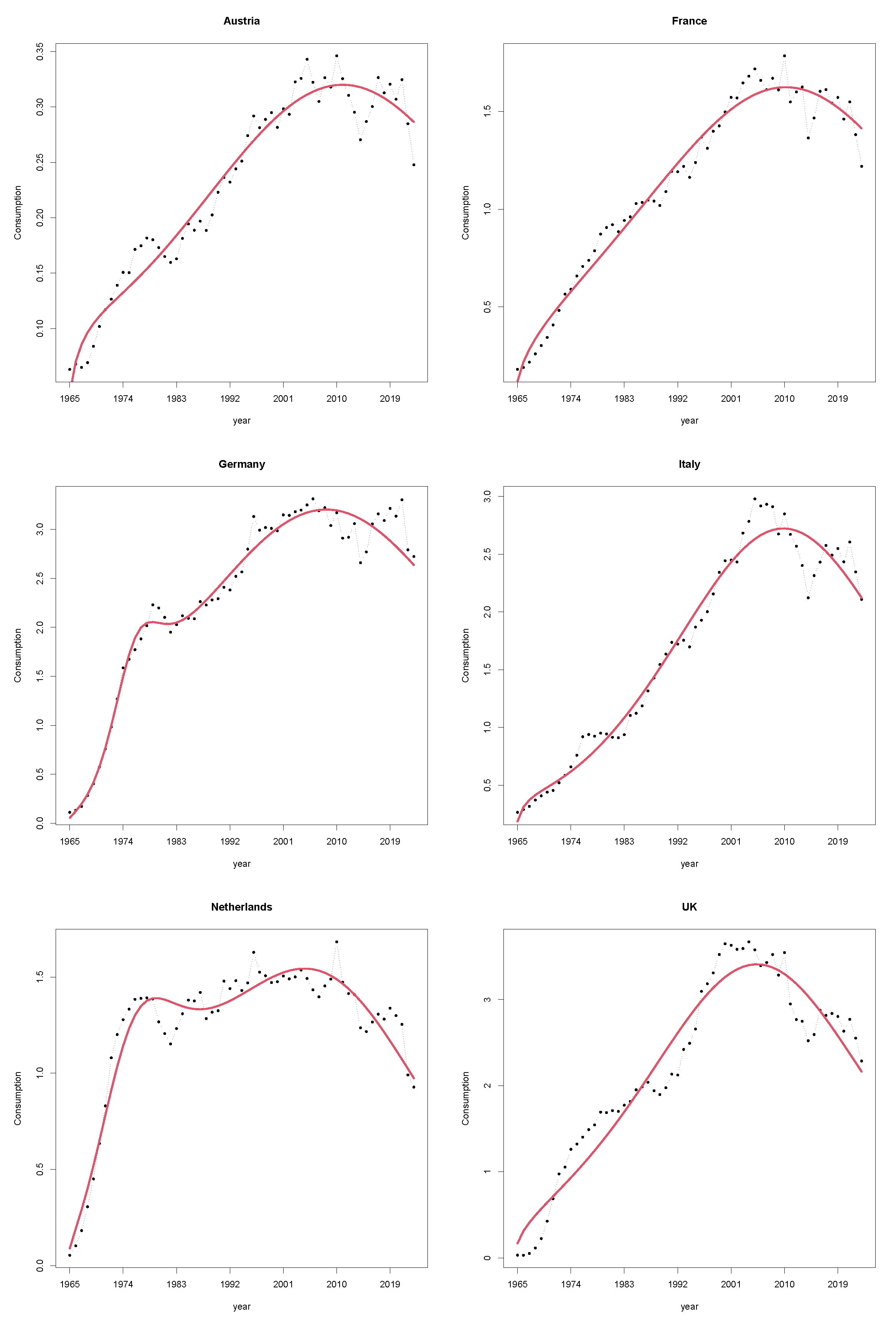
This work shows how combining innovation diffusion models—particularly the GGM—with ARIMAX provides a flexible framework for forecasting future gas consumption. This approach accounts for different temperature evolution scenarios and quantifies forecast uncertainty. As a general remark, we may say that our findings agree with the projected scenarios proposed by the IEA, according to which natural gas consumption is peaking and will decline in the future.

We have decided to focus on the major natural gas consumers in the European Union, considering them as paradigmatic examples of the complexity of energy markets. As reported in the IEA’s World Energy Outlook 2024, the European Union represents 6% of the world’s population and accounts for approximately 10% of global energy demand. The EU continues to be a clean energy leader; energy-related CO₂ emissions are declining, driven by increased electricity production from renewables, hydro, and nuclear power recovery, reduced industry emissions, and milder temperatures.

As a first step, we used the GGM to model the mean evolution of gas consumption in all of the selected countries, capturing the declining trend observed across all series. This modeling approach offered a parsimonious and interpretable way to describe the structural dynamics underlying gas consumption, where the observed decline may derive from policy-driven changes such as those promoted by the Fit for 55 package and the REPowerEU plan.

Additional policy initiatives have focused on enhancing the resilience of European gas markets, promoting solidarity, and mitigating extreme price spikes; for example, in July 2022 the EU adopted the European Gas Demand Reduction Plan, which provides best practices and guidance for reducing regional gas demand. These efforts include transitioning from gas use and towards renewables and cleaner energy sources in the industrial, power, and heating sectors.

Thanks to continued policy support for renewables, approximately 50 GW of wind and solar capacity was installed in the EU in 2022, representing a record high; according to the International Energy Agency, these additions offset the need for roughly 11 billion cubic meters of natural gas in the power sector, constituting the single most significant structural driver behind the EU’s recent decline in natural gas demand.

As a second step, ARIMAX modeling allowed us to produce point forecasts for Austria, France, Germany, Italy, the Netherlands, and the UK, suggesting a gradual reduction in consumption between 2024 and 2028. The same downward trend is generally followed by the upper and lower bounds of the produced predictive intervals. This clear-cut trend does not appear to stem from the smoothness of the temperature paths projected in CMIP6, which we adopted as covariates in our analysis, despite observed temperatures prior to 2023 tending to exhibit much more irregular fluctuations.

Indeed, similar conclusions have been reached when statistically modeling temperatures and using simulated paths for future temperatures from inferred models.

To extend the analysis, socioeconomic variables could be taken into account more explicitly by including them as covariates in the model rather than implicitly accounting for them, as in our GGM–ARIMAX framework. At the same time, one of the benefits of our proposed framework lies in its parsimony, which would be threatened by adding other parameters deriving from the inclusion of several covariates. Furthermore, our two-stage methodology can be easily used and implemented on different case studies referring to other countries by using publicly available energy consumption and temperature data. This potential for generalization is ensured by the basic requirements of the proposed approach in terms of both data and modeling complexity.

From a modeling point of view, a further interesting direction for future work is to infer both the GGM and ARIMAX model parameters in a Bayesian fashion, allowing both components to be integrated out with respect to the posterior when computing predictive distributions. This should ensure a more robust form of model averaging as well as the production of predictive intervals that are underpinned by a more comprehensive quantification of uncertainty.

References

1. Igliński, B.; Kiełkowska, U.; Mazurek, K.; Drużyński, S.; Pietrzak, M.B.; Kumar, G.; Veeramuthu, A.; Skrzatek, M.; Zinecker, M.; Piechota, G. Renewable energy transition in Europe in the context of renewable energy transition processes in the world. A review. Heliyon 2024, 10, e40997. [Google Scholar] [CrossRef]
2. Ding, L.; Zhao, Z.; Wang, L. Probability density forecasts for natural gas demand in China: Do mixed-frequency dynamic factors matter? Appl. Energy 2022, 312, 118756. [Google Scholar] [CrossRef]
3. Panek, W.; Włodek, T. Natural gas consumption forecasting based on the variability of external meteorological factors using machine learning algorithms. Energies 2022, 15, 348. [Google Scholar] [CrossRef]
4. Šebalj, D.; Mesarić, J.; Dujak, D. Predicting natural gas consumption—A literature review. In Proceedings of the Central European Conference on Information and Intelligent Systems, Varazdin, Croatia, 27–29 September 2017. [Google Scholar]
5. Liu, J.; Wang, S.; Wei, N.; Chen, X.; Xie, H.; Wang, J. Natural gas consumption forecasting: A discussion on forecasting history and future challenges. J. Nat. Gas Sci. Eng. 2021, 90, 103930. [Google Scholar] [CrossRef]
6. Sen, D.; Hamurcuoglu, K.I.; Ersoy, M.Z.; Tunç, K.M.; Günay, M.E. Forecasting long-term world annual natural gas production by machine learning. Resour. Policy 2023, 80, 103224. [Google Scholar] [CrossRef]
7. Ding, J.; Zhao, Y.; Jin, J. Forecasting natural gas consumption with multiple seasonal patterns. Appl. Energy 2023, 337, 120911. [Google Scholar] [CrossRef]
8. Li, N.; Wang, J.; Liu, R.; Zhong, Y. What is the short-term outlook for the EU’s natural gas demand? Individual differences and general trends based on monthly forecasts. Environ. Sci. Pollut. Res. 2022, 29, 78069–78091. [Google Scholar] [CrossRef]
9. Soldo, B. Forecasting natural gas consumption. Appl. Energy 2012, 92, 26–37. [Google Scholar] [CrossRef]
10. Hafezi, R.; Alipour, M.; Wood, D.A.; Moghaddam, N.B. Natural gas demand prediction: Methods, time horizons, geographical scopes, sustainability issues, and scenarios. In Sustainable Natural Gas Reservoir and Production Engineering; Elsevier: Amsterdam, The Netherlands, 2022; pp. 29–53. [Google Scholar]
11. Dawid, A.P. Present Position and Potential Developments: Some Personal Views: Statistical Theory: The Prequential Approach. J. R. Stat. Soc. Ser. A (Gen.) 1984, 147, 278–292. [Google Scholar] [CrossRef]
12. Gneiting, T.; Balabdaoui, F.; Raftery, A.E. Probabilistic forecasts, calibration and sharpness. J. R. Stat. Soc. Ser. B Stat. Methodol. 2007, 69, 243–268. [Google Scholar] [CrossRef]
13. Gneiting, T.; Katzfuss, M. Probabilistic Forecasting. Annu. Rev. Stat. Its Appl. 2014, 1, 125–151. [Google Scholar] [CrossRef]
14. Hyndman, R.J.; Athanasopoulos, G. Forecasting: Principles and Practice; OTexts: Melbourne, Australia, 2018. [Google Scholar]
15. Guseo, R.; Guidolin, M. Modelling a dynamic market potential: A class of automata networks for diffusion of innovations. Technol. Forecast. Soc. Change 2009, 76, 806–820. [Google Scholar] [CrossRef]
16. Ciais, P.; Bréon, F.M.; Dellaert, S.; Wang, Y.; Tanaka, K.; Gurriaran, L.; Françoise, Y.; Davis, S.J.; Hong, C.; Penuelas, J.; et al. Impact of Lockdowns and Winter Temperatures on Natural Gas Consumption in Europe. Earth Future 2022, 10, e2021EF002250. [Google Scholar] [CrossRef]
17. Botzen, W.W.; Nees, T.; Estrada, F. Temperature effects on electricity and gas consumption: Empirical evidence from Mexico and projections under future climate conditions. Sustainability 2020, 13, 305. [Google Scholar] [CrossRef]
18. Guseo, R.; Dalla Valle, A.; Guidolin, M. World Oil Depletion Models: Price effects compared with strategic or technological interventions. Technol. Forecast. Soc. Change 2007, 74, 452–469. [Google Scholar] [CrossRef]
19. Guidolin, M.; Mortarino, C. Cross-country diffusion of photovoltaic systems: Modelling choices and forecasts for national adoption patterns. Technol. Forecast. Soc. Change 2010, 77, 279–296. [Google Scholar] [CrossRef]
20. Bass, F.M. A new product growth for model consumer durables. Manag. Sci. 1969, 15, 215–227. [Google Scholar] [CrossRef]
21. Guidolin, M.; Guseo, R. The German energy transition: Modeling competition and substitution between nuclear power and Renewable Energy Technologies. Renew. Sustain. Energy Rev. 2016, 60, 1498–1504. [Google Scholar] [CrossRef]
22. Guidolin, M.; Alpcan, T. Transition to sustainable energy generation in Australia: Interplay between coal, gas and renewables. Renew. Energy 2019, 139, 359–367. [Google Scholar] [CrossRef]
23. Bessi, A.; Guidolin, M.; Manfredi, P. The role of gas on future perspectives of renewable energy diffusion: Bridging technology or lock-in? Renew. Sustain. Energy Rev. 2021, 152, 111673. [Google Scholar] [CrossRef]
24. Guidolin, M.; Manfredi, P. Innovation diffusion processes: Concepts, models, and predictions. Annu. Rev. Stat. Its Appl. 2023, 10, 451–473. [Google Scholar] [CrossRef]
25. Guidolin, M. Innovation Diffusion Models: Theory and Practice; John Wiley & Sons: Hoboken, NJ, USA, 2023. [Google Scholar]
26. Petropoulos, F.; Apiletti, D.; Assimakopoulos, V.; Babai, M.Z.; Barrow, D.K.; Taieb, S.B.; Bergmeir, C.; Bessa, R.J.; Bijak, J.; Boylan, J.E.; et al. Forecasting: Theory and Practice. Int. J. Forecast. 2022, 38, 705–871. [Google Scholar]
27. Bierens, H.J. Topics in Advanced Econometrics: Estimation, Testing, and Specification of Cross-Section and Time Series Models; Cambridge University Press: Cambridge, UK, 1994. [Google Scholar]
28. Bierens, H.J. Armax model specification testing, with an application to unemployment in the Netherlands. J. Econom. 1987, 35, 161–190. [Google Scholar] [CrossRef]
29. Box, G.E.P.; Jenkins, G.M.; Reinsel, G.C. Time Series Analysis: Forecasting and Control; John Wiley & Sons: Hoboken, NJ, USA, 2008. [Google Scholar]
30. Harrison, J.; West, M. Bayesian Forecasting and Dynamic Models; Springer: New York, NY, USA, 1987. [Google Scholar]
31. Petris, G.; Petrone, S.; Campagnoli, P. Dynamic Linear Models with R; Springer: Berlin/Heidelberg, Germany, 2009. [Google Scholar]
32. Shumway, R.H.; Stoffer, D.S. Time Series Analysis and Its Applications with R Examples; Springer: Berlin/Heidelberg, Germany, 2017. [Google Scholar]
33. Prado, R.; West, M. Time Series: Modeling, Computation, and Inference; CRC Press: Boca Raton, FL, USA, 2010. [Google Scholar]
34. Zanghi, F.; Savio, A.; Ziliotto, F.; Bessi, A. Package DIMORA: Diffusion Models R Analysis. 2023. Available online: https://cran.r-project.org/web/packages/DIMORA/index.html (accessed on 18 May 2025).
35. Alonzo Matamoros, A.; Cruz Torres, C.; Dala, A.; Hyndman, R.; O’Hara-Wild, M. Package bayesforecast: Bayesian Time Series Modeling with Stan. 2022. Available online: https://CRAN.R-project.org/package=bayesforecast (accessed on 18 May 2025).
36. Durhasan, T.; Pinar, E.; Uluocak, I.; Bilgili, M. Future forecast of global mean surface temperature using machine learning and conventional time series methods. Theor. Appl. Climatol. 2025, 156, 17. [Google Scholar] [CrossRef]
Figure 1. Yearly gas consumption (dotted lines) by country from 1965 to 2023.
Forecasting 07 00023 g001
Figure 2. Annual average mean surface air temperature (dotted lines) by country from 1965 to 2023.
Forecasting 07 00023 g002
Figure 3. Estimated means of gas consumption (red solid lines) and actual consumption (dotted lines) from 1965 to 2023 via frequentist estimate of GGMs based on the whole time series.
Forecasting 07 00023 g003
Figure 4. Residuals from GGM fit (dotted lines).
Forecasting 07 00023 g004
Figure 5. Dynamic one-step-ahead forecasts of yearly gas consumption from 1996 to 2023 (red solid line) and predictive intervals of 0.95 (blue dashed line) and 0.99 (light blue dashed line) levels.
Forecasting 07 00023 g005aForecasting 07 00023 g005b
Figure 6. Estimated means of gas consumption levels from 1965 to 2023, summing frequentist estimates of the GGM component and posterior means of the residuals’ expectations based on ARIMAX model fitting and using the whole time series.
Forecasting 07 00023 g006
Figure 7. Forecasted consumption levels from 2024 to 2028 (dashed lines) and 0.95 -predictive intervals (dotted lines) under different scenarios (SSPs) based on GGM and and ARIMAX model fitting for the filtered series and temperature projections in Table A4.
Forecasting 07 00023 g007
Figure 8. Forecasted consumption levels from 2024 to 2028 (dashed lines) and 0.95 -predictive intervals (dotted lines) under different scenarios (SSPs) based on GGM and and ARIMAX model fitting for the filtered series and temperature projections in Table A4.
Forecasting 07 00023 g008