Abstract
Water temperature is a fundamental parameter influencing a range of biotic and abiotic processes occurring within various components of the hydrosphere. This study presents a multi-step, data-driven predictive modeling framework to estimate water temperatures for the period 2021–2100 in three aquatic environments in Central Europe: the Odra River, the Szczecin Lagoon, and the Baltic Sea. The framework integrates Bayesian Model Averaging (BMA), Random Sample Consensus (RANSAC) regression, Gradient Boosting Regressor (GBR), and Random Forest (RF) machine learning models. To assess the performance of the models, the coefficient of determination (R2), mean absolute error (MAE), and root mean square error (RMSE) were used. The results showed that the application of statistical downscaling methods improved the prediction of air temperatures with respect to the BMA. Moreover, the RF method was used to predict water temperature. The best model performance was obtained for the Baltic Sea and the lowest for the Odra River. Under the SSP2-4.5 and SSP5-8.5 scenario-based simulations, projected air temperature increases in the period 2021–2100 could range from 1.5 °C to 1.7 °C and 4.7 to 5.1 °C. In contrast, the increase in water temperatures by 2100 will be between 1.2 °C and 1.6 °C (SSP2-4.5 scenario) and between 3.5 °C and 4.9 °C (SSP5-8.5).
1. Introduction
The hydrosphere is one of Earth’s geosystems that, through the water cycle, connects other environmental components via the exchange of energy and matter. It is generally divided into saline and freshwater bodies, with coastal zones also featuring transitional elements. Elements of the hydrographic network in the immediate vicinity of the sea are shaped both by the sea itself and by processes originating from the land [1]. Different components of the hydrosphere, functioning under specific geological and climatic conditions, exhibit varying characteristics primarily determined by the fundamental properties of water. One such key parameter is temperature, whose distribution and fluctuations significantly influence both biotic and abiotic processes. Persistently warm water temperatures (e.g., coastal lagoons in New England) have significantly reduced eelgrass density and extended the interval between the emergence of new leaves [2]. Studies conducted in the Thau Lagoon in the Mediterranean have shown that water temperature is the primary factor influencing community diversity and seasonal succession from winter to spring [3]. In the Barents Sea, water temperature recorded 10 months earlier was identified as the only significant predictor of zooplankton population characteristics [4]. An increase in ambient noise levels (Atlantic, North Carolina), caused by higher water temperatures, has ecological implications for signal detection, communication, and navigation [5]. In the Seine River, water warming reduced dissolved oxygen levels and increased phytoplankton biomass during the growth season [6]. Additionally, changes in water temperature in the Jinsha River, following the construction of a dam, may shift the primary spawning period of native fish in the river’s lower course to early March–late July or late March–early August [7].
Elements of the hydrographic network undergo constant transformations of varying intensity, determined by both natural and anthropogenic factors [8]. The close relationship between the atmosphere and water makes the latter highly sensitive to changes occurring in the atmosphere [9]. Nowadays, global warming stands as one of the greatest challenges facing humanity. In the context of this issue, it significantly influences the thermal properties of seas, lagoons, rivers, and lakes [10,11,12]. Referring to the previously mentioned division (saltwater, freshwater, and transitional waters), each of these environments will undergo transformations driven by rising temperatures. Particularly interesting in this regard are lagoons, whose characteristics are shaped by both inflows from land and interactions with the sea. As noted by Zannella et al. [13], coastal lagoons are crucial for recreation, ecology, and commerce, yet they are often highly vulnerable to both natural and anthropogenic changes. Due to climate change, the thermal sensitivity of coastal water bodies remains poorly understood [14]. In water sciences, there is a growing focus on predicting future changes, which, in terms of temperature dynamics, is reflected in studies covering various elements of these ecosystems [15,16,17].
In Poland, studies on water temperature prediction are scarce and primarily focus on lakes and rivers [18,19]. The existing results are concerning, indicating a continued warming of aquatic ecosystems. Against this backdrop, there is a need to broaden knowledge on future changes in various aspects, particularly concerning the sea and coastal lagoons. The aim of this article is to explore potential future changes in water temperature under scenario-based modeling simulations across three aquatic environments: a river (Odra River), a lagoon (Szczecin Lagoon), and the sea (Baltic Sea, Pomeranian Bay) in northwestern Poland. This region has been the subject of numerous environmental studies [20,21,22], and the research presented here expands the current understanding by highlighting the direction and scale of thermal regime changes in selected components of the hydrosphere. The innovative aspect of this study lies in identifying the direction and scale of changes in the thermal regime of selected elements of the hydrosphere that have not been previously analyzed. A strong point of the conducted research is the use of minimal input assumptions in the modeling process, based on a widely accessible parameter—air temperature.
2. Materials and Methods
2.1. Study Objects
The Odra River is the second-longest river in Poland (855 km). In terms of drainage basin area, it ranks 15th in Europe (118,000 km2). The river has an average discharge of 500 m3/s, and its hydrological regime in the lower course is classified as nival medium [23]. The outflow of the spring months is 130 to 180% of the average annual outflow [23]. The river flows into the Szczecin Lagoon, which covers an area of 686.9 km2 with an average depth of 3.8 m [24]. The lagoon is divided into two parts: the Great Lagoon (eastern part) and the Small Lagoon (western part) [25]. The hydrological and hydrochemical conditions of the lagoon are mainly shaped by the influence of the Odra River and the periodic backflow of brackish waters. The water masses flowing through the canal connecting the Szczecin Lagoon with the Baltic Sea are characterized by high dynamics and variable flow rates [26]. The Szczecin Lagoon plays a significant role in Poland’s maritime economy [24], serving as the route for the waterway leading to the Port of Szczecin—a key transit hub for maritime, river, and land transportation. The marine station is located in the Baltic Sea (Figure 1) within the Pomeranian Bay, which has a surface area of approximately 6000 km2 and an average depth of 13 m. The seafloor features diverse topography [27]. Together, the lower Odra River, the Szczecin Lagoon, and the Pomeranian Bay (Baltic Sea) form a hydrographic system with estuarine characteristics, where the mixing of marine and river waters occurs with variable dynamics [27].
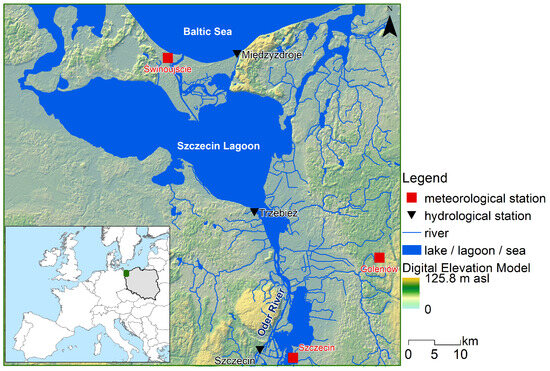
Figure 1.
Location of research objects.
2.2. Materials
The study utilized data from 2009 to 2020 on daily water temperatures from three stations: Szczecin (river station), Trzebież (lagoon station), and Międzyzdroje (sea station). The data were provided by the Institute of Meteorology and Water Management—National Research Institute. Water temperature measurements were taken at a depth of 0.4 m below the water surface at 6 UTC. During the same period, air temperature data were collected for three stations: Szczecin, Goleniów, and Świnoujście. These air temperature measurements were conducted as part of the standard meteorological monitoring in Poland and WMO, which includes measurements at a height of 2 m above ground level.
2.3. Methods
This study employs a multi-step modeling framework to predict water temperatures in river, lagoon, and sea environments by integrating Bayesian Model Averaging (BMA), statistical downscaling, and machine learning (ML) techniques. The approach ensures robust climate predictions by leveraging multiple global climate models (GCMs) while minimizing the uncertainties associated with individual models. Each component of the methodology follows a sequential process to enhance accuracy, maintain physical consistency, and improve the spatial and temporal resolution of temperature predictions.
2.3.1. Bayesian Model Averaging (BMA) for Air Temperature Aggregation
Bayesian Model Averaging (BMA) is used to aggregate air temperature projections from multiple GCMs as listed in Table 1.

Table 1.
List of Global Climate Models (GCMs) used in Bayesian Model Averaging (BMA).
Since individual GCMs exhibit systematic biases and varying degrees of uncertainty, BMA assigns probabilistic weights to each model based on its predictive performance. The ensemble used in this study consists of nine GCMs sourced from the Coupled Model Intercomparison Project Phase 6 (CMIP6), representing contributions from various climate research institutions globally. To ensure uniformity, all temperature projections were bias-corrected using quantile mapping, as detailed in Section 2.3 (Statistical Downscaling), before incorporation into the modeling framework.
Each model provides its surface temperature covering the period from 2009 to 2100, with data from 2009 to 2014 derived from historical simulations and data from 2015 onward based on the scenario-driven future. These predictions are then adjusted to a similar spatial resolution to maintain uniformity across the group. The re-gridding procedure utilizes linear interpolation to map the model outputs onto a predetermined grid of latitude and longitude, enabling straightforward comparison.
This study uses BMA [37] to combine projections from nine GCMs. BMA is a statistical framework that allows for the combination of predictions made by various models using probability theory. The principle behind this approach is Bayes’ theorem, which can be mathematically formulated in the context of model averaging as follows:
The expression represents the posterior probability of model Mi given the data y. Similarly, denotes the likelihood of the data y under model Mi. The term refers to the prior probability of model Mi, while p(y) represents the marginal likelihood of the data y and serves as a normalizing constant.
The BMA predictive distribution for a new observation is calculated by taking a weighted average of the predictive distributions from each model.
The equation involves the predictive distribution, , which represents the probability distribution of the new observation given the model . Additionally, serves as the weight for model , and it is calculated as explained earlier.
The ensemble of climate models provides a combined BMA prediction for the surface temperature (T) at a specific grid point (x,y) and time (t).
Ti (x,y,t) represents the forecast generated by model i, whereas wi (x,y,t) is the BMA weight assigned to model i at grid point (x,y) and time t. This weight is determined based on the posterior probability p(Mi∣y), which is particular to the given place and time.
2.3.2. Statistical Downscaling of Air Temperature
Given that GCMs operate at coarse spatial resolutions, their direct application to local-scale temperature prediction is limited. To bridge this gap, a statistical downscaling framework is implemented, which refines the BMA-derived air temperature projections into high-resolution, location-specific temperature predictions. This downscaling approach preserves both long-term climate trends and local-scale variability by incorporating quantile mapping transformation, robust regression, and extreme value handling techniques [38].
The downscaling procedure begins with the quantile mapping transformation of the BMA temperatures, where each temperature value is normalized using the mean and standard deviation from the calibration period (2009–2014) [39]. This transformation is expressed as follows:
where represents the normalized or scaled version of the BMA temperature, refers to the raw temperature projections obtained from Bayesian Model Averaging (BMA), before any transformations or corrections. μBMA and σBMA are the mean and standard deviation of the calibration dataset, ensuring that the temperature values are scaled to a standardized range, and ε is a small constant to prevent division by zero. After this transformation, the scaled temperatures are further mapped to a normal distribution using an adaptive quantile transformer, ensuring that the distribution of downscaled temperatures maintains statistical consistency with observed records [40].
Once the quantile-mapped temperatures are generated, Random Sample Consensus (RANSAC) regression is applied to establish a robust relationship between the transformed BMA temperatures and observed air temperatures. RANSAC is particularly effective in handling outliers and ensuring robust statistical relationships, making it well suited for climate applications where extreme values are common [41]. The downscaled temperature values are modeled using the equation:
where represents the final adjusted temperature value at the local scale, obtained after applying RANSAC regression to the mapped BMA temperatures. α and β are regression coefficients, and represents the statistically adjusted temperature values after quantile mapping transformation is applied to . The RANSAC implementation uses 30% of the calibration data as a minimum sample size, with a maximum of 200 trials to ensure optimal coefficient determination.
For handling extreme temperature events, a scaling factor adjustment is applied whenever temperature anomalies exceed two standard deviations from the mean. This ensures that extreme climate variations, such as heatwaves and cold anomalies, are properly represented in the downscaled data [42]. To enhance the residual correction process, a Gradient Boosting Regressor (GBR) is employed, effectively capturing non-linear relationships that may not be well represented by linear regression models [43]. GBR is an ensemble learning technique that builds a sequence of weak learners (typically decision trees), where each subsequent model focuses on minimizing the residual errors of the previous iteration. Mathematically, GBR optimizes a function F(x) by iteratively refining it through gradient descent in function space [44]. The prediction function at iteration mmm is updated as follows:
where is the updated prediction function after mmm iterations, is the previous iteration’s prediction function, is the learning rate, which controls the contribution of each new tree, and is the weak learner (a decision tree) trained on the residuals from the previous step.
For this study, the GBR model is optimized with 100 estimators, a maximum depth of 4, and a learning rate of 0.1 to ensure a balance between predictive accuracy and computational efficiency. The use of GBR ensures that complex temperature patterns, which may not be captured by simple linear transformations, are effectively represented in the downscaled air temperature data. This residual correction step significantly improves model performance by reducing systematic biases and enhancing the robustness of temperature predictions, particularly in capturing extreme temperature variations [45].
2.3.3. Machine Learning for Water Temperature Prediction
Water temperature predictions are generated using Random Forest (RF) machine learning models, with separate models developed for rivers, estuaries, and seas. Each model is designed to account for the specific environmental dynamics governing temperature variations in these aquatic systems. The RF model is chosen for its ability to handle complex, non-linear relationships while maintaining high predictive accuracy [46]. The final water temperature predictions are obtained by averaging the outputs from an ensemble of 100 decision trees, each trained on different subsets of input data. The final prediction is computed using the following equation:
where T represents the total number of decision trees and is the prediction from each tree.
For river and lagoon temperature modeling, ten key predictive features derived from air temperature data are incorporated into the RF model. These include short-term (15-day) and long-term (60-day) moving averages, which help capture recent and seasonal temperature trends. These are computed as follows:
Seasonal variability is represented through harmonic functions, capturing annual and semi-annual temperature cycles:
The sea environment model extends the framework developed for river and lagoon temperature predictions by incorporating sea surface temperature (SST) data from the NOAA OI SST V2 High-Resolution Dataset [47,48]. Unlike river and lagoon systems, where temperature variations are primarily driven by local atmospheric conditions and freshwater inflows, sea water temperature is influenced by a combination of atmospheric forcing, ocean circulation, and large-scale climate variability [49]. To capture these interactions, the model integrates additional SST-specific predictors beyond the base air temperature features. These include SST anomalies, SST gradients, and Air–SST interaction terms, which collectively enhance the model’s ability to represent complex ocean–atmosphere dynamics.
SST anomalies () quantify deviations of sea surface temperature from its climatological mean. This helps to identify warming or cooling trends relative to long-term averages. This feature is crucial for detecting climate-driven variations in oceanic thermal patterns, including marine heatwaves, ENSO (El Niño–Southern Oscillation) effects, and regional upwelling events [50]. The SST anomaly is computed as follows:
where SST represents the observed sea surface temperature at a given location and time, and is the long-term mean SST for the same location and calendar day, averaged over multiple years.
SST gradients () describe the rate of temperature change over time, which is essential for understanding short-term oceanic thermal variability, heat advection, and mixing processes. Gradients help detect sudden shifts in SST, such as those caused by storms, ocean currents, or atmospheric heat exchanges [51]. The SST gradient is computed as follows:
where is the sea surface temperature at the current time step, is the sea surface temperature at the previous time step, and represents the time interval (typically daily or monthly, depending on data resolution).
The interaction between air temperature and SST plays a critical role in determining energy exchanges at the air–sea interface. The inclusion of an Air–SST interaction term allows the model to capture how atmospheric conditions influence ocean temperatures and vice versa [52]. This interaction is particularly relevant for understanding ocean heat flux, surface evaporation rates, and cloud formation processes. The Air–SST interaction term is defined as follows:
where represents the local air temperature, and is the deviation of SST from its climatological mean.
2.3.4. Model Evaluation
The dataset covering the period 2009–2020 was divided into training and validation subsets. Specifically, 80% of the data (2009–2018) was used for model training, during which 10-fold cross-validation was applied to optimize model performance and prevent overfitting. The remaining 20% (2019–2020) was reserved as an independent validation set to assess the generalization capability of the final model. To assess the performance and accuracy of the temperature prediction models developed in this study, three key evaluation metrics are used: the coefficient of determination (R2), mean absolute error (MAE), and root mean square error (RMSE). The models were evaluated using data from the period 2009–2014. These metrics provide a comprehensive evaluation of the model’s ability to reproduce observed temperature variations across river, lagoon, and sea environments.
R2 measures the proportion of variance in observed temperature values that is explained by the model predictions. It is defined as follows:
MAE quantifies the average magnitude of errors between observed and predicted temperatures, regardless of direction. It is computed as follows:
RMSE measures the standard deviation of residual errors, placing greater emphasis on larger errors due to squaring deviations before averaging. It is calculated as follows:
where represents the observed temperature, represents the predicted temperature, is the mean observed temperature, and n is the total number of observations.
2.3.5. Analysis of the Direction and Rate of Change of Water Temperatures
Analysis of the direction and magnitude of changes in average annual water temperatures in the Odra River, the Szczecin Lagoon, and the Baltic Sea over the period 2021–2100 was performed using Mann–Kendall [53] and Sen [54] tests. The former allowed for the assessment of the significance of changes in water temperature, while the latter allowed for the determination of the magnitude of the change. Mann–Kendall and Sen tests were conducted using the modified mk package in R 3.5.1 developed by Patakamuri and O’Brien [55]. The Mann–Kendall test was performed at a significance level of 0.05.
3. Results
Figure 2 presents a comparison of observed and predicted air temperatures using the Bayesian Model Averaging (BMA) method for Szczecin, Goleniów, and Świnoujście meteorological stations from 2009 to 2020.
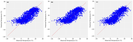
Figure 2.
Comparison of observed and predicted air temperature (°C) using the BMA method for (a) Szczecin, (b) Goleniów, and (c) Świnoujście meteorological stations in the period 2009–2014.
The scatter plots illustrate a strong positive correlation between observed and predicted values. While the BMA method generally performs well in estimating air temperature across all meteorological stations, some deviations are noticeable, particularly at extreme temperature ranges. In the case of air temperature at Szczecin station (Figure 2a), the predictions closely follow the observed values, though the model tends to underestimate higher temperatures and overestimate lower temperatures. Similarly, for air temperatures at Goleniów station (Figure 2b), the correlation between observed and predicted temperatures remains strong, with slightly lower prediction errors compared to Szczecin meteorological station. This improved performance could be attributed to more stable air temperature in the region of Szczecin Lagoon. However, some scatter is observed at both lower and higher temperature ranges. At Świnoujście station (Figure 2c), the predictions align well with observations, with a slightly more constrained spread of data points compared to Szczecin station. However, deviations persist, particularly in colder temperature ranges, where the model tends to underestimate values.
Figure 3 presents a comparison of observed and predicted air temperatures (°C) using the statistical downscaling method for Szczecin, Goleniów, and Świnoujście meteorological stations from 2009 to 2020.
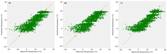
Figure 3.
Comparison of observed and predicted air temperature (°C) using the statistical downscaling method for (a) Szczecin, (b) Goleniów, and (c) Świnoujście meteorological stations in the period of 2009–2014.
The scatter plots indicate a strong correlation between observed and predicted values. The statistical downscaling method appears to perform well in estimating air temperature across the different meteorological stations, though some discrepancies are evident, particularly at extreme temperature ranges. At Szczecin meteorological station (Figure 3a), the predicted air temperatures closely align with observations, but there is a tendency for the model to slightly underestimate higher temperatures and overestimate lower temperatures. In Goleniów station (Figure 3b), the predictions also show a strong correlation with observed values, though the spread of data points suggests some degree of uncertainty. Notably, a step-like pattern is observed in the predicted values, where plateaus appear despite variation in observed temperatures. This effect arises from the quantile mapping transformation applied during bias correction, which, when performed on a relatively short calibration period (2009–2014), can result in discretized output values due to limited resolution in the empirical distribution. Additionally, the use of RANSAC regression—which emphasizes robust fitting—may reinforce this grouping by down-weighting outliers. At Świnoujście station (Figure 3c), the predictions demonstrate a tight correlation with observations, with less scatter compared to Szczecin meteorological station. However, minor deviations are noticeable, particularly at lower temperatures, where the model slightly underestimates values.
Table 2 presents a comparative assessment of the performance of Bayesian Model Averaging (BMA) and statistical downscaling methods in predicting air temperature across the different meteorological stations (Szczecin, Goleniów, and Świnoujście) in the period of 2009–2020.
Table 2.
Comparison of BMA and statistical downscaling performance for air temperature prediction in the analyzed meteorological stations in the period of 2009–2020.
The performance metrics considered include the coefficient of determination (R2), mean absolute error (MAE), and root mean square error (RMSE). The results indicate that the statistical downscaling method consistently outperforms the BMA method across all meteorological stations. In terms of R2, the statistical downscaling approach demonstrates a significantly higher correlation between observed and predicted air temperatures, with values of 0.85, 0.86, and 0.87 for Szczecin, Goleniów, and Świnoujście meteorological stations, respectively, compared to the lower values of 0.63, 0.62, and 0.70 obtained using BMA. This suggests that statistical downscaling provides a more reliable estimation of air temperature variations. Similarly, the MAE values for statistical downscaling (ranging from 2.15 °C to 2.43 °C) are notably lower than those for BMA (ranging from 3.21 °C to 3.89 °C), indicating that statistical downscaling yields more precise predictions with fewer deviations from observed temperatures. The RMSE values further reinforce this trend, with statistical downscaling demonstrating lower errors across all meteorological stations. For instance, in Świnoujście station, statistical downscaling achieves an RMSE of 2.73 °C compared to 4.12 °C for BMA, underscoring its superior predictive accuracy.
Figure 4 presents the learning curves for the machine learning models predicting water temperature in (a) river, (b) lagoon, and (c) sea environments.
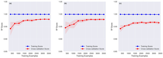
Figure 4.
Learning curves for machine learning models predicting water temperature in (a) river, (b) lagoon, and (c) and sea environments.
The figure illustrates the relationship between the number of training examples and the model’s performance, as measured by R2. The shaded region around the cross-validation score represents its standard deviation, reflecting the uncertainty in model performance. Across all three hydrological stations, the training score remains consistently high (R2 ≈ 1.0), indicating that the models fit the training data almost perfectly. This behavior is characteristic of Random Forest models, which are capable of overfitting small datasets due to their flexibility and ensemble structure. This perfect training score phenomenon occurs because Random Forests can exactly memorize training data, achieving zero training error when trees are sufficiently deep [44]. As Breiman [46] demonstrated in his seminal paper, Random Forests consist of multiple decision trees, each trained on bootstrapped samples of the data and a random subset of features. With sufficient trees (in this case, 100) and adequate depth (max_depth = 15 in the implementation), the model effectively memorizes the training data when the sample size is small [56]. This occurs because individual trees can grow deeply enough to capture noise patterns unique to each observation, while the ensemble averaging prevents high variance in predictions [57]. Unlike linear models, tree-based models do not make assumptions about the underlying data distribution and can thus represent complex, non-linear relationships even with minimal training examples [58]. The high training score and initial gap between training and cross-validation scores illustrate this characteristic overfitting tendency, which diminishes as more training examples introduce greater variability and prevent the model from memorizing individual data points. However, the cross-validation score starts lower but steadily increases as more training examples are added, demonstrating the benefits of additional data in improving generalization performance. The initial gap between training and validation scores suggests a degree of overfitting, which progressively reduces as more training data are included. For river water temperature predictions (Figure 4a), the cross-validation score begins around R2 ≈ 0.93 with a small training set and gradually improves, stabilizing at approximately R2 ≈ 0.97 as the number of training samples increases. A similar trend is observed in lagoon water temperature predictions (Figure 4b), where the cross-validation score starts slightly lower but follows a comparable trajectory, converging at around R2 ≈ 0.97. The sea water temperature model (Figure 4c) demonstrates a high generalization performance, with the cross-validation score reaching approximately R2 ≈ 0.96 as the training data expand. Although the model benefits from incorporating sea surface temperature (SST) predictors, the cross-validation score remains slightly lower than those for the river and lagoon environments, likely due to greater variability and complexity in ocean–atmosphere interactions. This superior performance is likely attributed to the inclusion of sea surface temperature (SST) as a predictor, which enhances the model’s ability to capture the greater thermal inertia and stability of ocean temperatures, making sea water temperature variations more predictable compared to river and lagoon systems.
To further assess model generalization and reduce the risk of overfitting, a leave-one-year-out cross-validation (LOYOCV) scheme was implemented across the 2009–2018 calibration period. In this procedure, each model was trained on all years except one and evaluated on the held-out year, iteratively. This approach allowed for an independent assessment of predictive skill across temporally disjointed subsets. The mean cross-validated R2 scores were 0.96 for the sea, 0.84 for the lagoon, and 0.83 for the river. Corresponding mean absolute errors (MAE) ranged from 0.94 °C to 2.60 °C, and RMSE values ranged from 1.23 °C to 3.26 °C across systems. These results suggest that the models can maintain strong predictive performance when tested against unseen annual conditions, within the limitations of the short calibration window. Detailed metrics and scatterplots for each water type are provided in the supplementary materials (Figures S1–S6).
Overall, the learning curves suggest that the models benefit from larger training datasets, as evidenced by the rising cross-validation scores. The convergence of training and validation scores at higher sample sizes indicates that the models generalize well and that overfitting is mitigated as more data become available. These results confirm the robustness of the proposed machine learning framework for water temperature prediction across different aquatic environments.
Figure 5 presents a comparison of observed and predicted water temperatures (°C) using the Random Forest method for river, lagoon, and sea environments from 2009 to 2020.
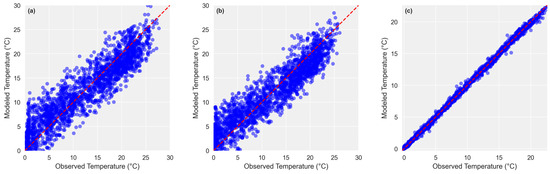
Figure 5.
Comparison of observed and predicted water temperatures (°C) using the RF method for (a) river, (b) lagoon, and (c) sea water temperatures in the period of 2009–2014.
The scatter plots illustrate a strong correlation between observed and predicted values. For river water temperature (Figure 5a), the predictions generally align with observations, though notable deviations occur, particularly at higher temperatures, indicating some limitations in model precision under extreme conditions. For lagoon water temperature (Figure 5b), the predictions show moderate agreement with observations, with reduced scatter compared to previous methods but still some dispersion across the range. The strongest correlation is observed in sea water temperature predictions (Figure 5c), where the data points are tightly clustered along the 1:1 reference line. This suggests that the RF method is particularly effective in marine environments, likely due to the more stable thermal regime and the inclusion of SST-specific predictors that enhance model performance.
Table 3 presents the performance metrics of the Random Forrest (RF) method for water temperature prediction across river, lagoon, and sea environments from 2009 to 2014.
Table 3.
Comparison of RF performance for water temperature prediction across different water types during 2009–2014.
The evaluation is based on the coefficient of determination (R2), mean absolute error (MAE), and root mean square error (RMSE), which provide insights into the accuracy and reliability of the RF predictions. The results indicate that the RF method performs exceptionally well across all water types, with consistently high R2 values and low error metrics. For river and lagoon environments, the R2 values of 0.83 and 0.84, respectively, demonstrate a strong correlation between observed and predicted water temperatures. The MAE values (2.58 °C for rivers and 2.43 °C for estuaries) and RMSE values (3.24 °C and 3.02 °C, respectively) indicate a notable reduction in error. These results demonstrate the strong performance of the Random Forest model in predicting dynamic water temperature variations, as reflected by the relatively low error metrics across all three aquatic environments.
The most significant improvement is observed for sea water temperature, where the RF method achieves an R2 of 0.98, indicating an almost perfect fit between observed and predicted values. The MAE (0.18 °C) and RMSE (0.26 °C) are remarkably low, further demonstrating the high accuracy of ML in predicting sea water temperature. This is likely due to the relatively stable thermal properties of the ocean, which the RF model can effectively learn and reproduce.
Figure 6 presents the historical (2009–2020) air temperature (°C) for river, lagoon, and sea environments based on observation and projections based on statistical downscaling under two Shared Socioeconomic Pathways (SSP2-4.5 and SSP5-8.5) from 2021 to 2100.
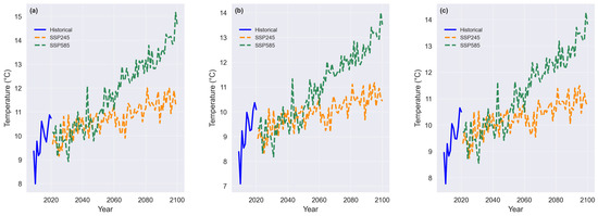
Figure 6.
Yearly average air temperature (°C) for (a) Szczecin, (b) Goleniów, and (c) Świnoujście locations, based on historical observations (2009–2020) and projections (2021–2100) under SSP2-4.5 and SSP5-8.5 scenarios.
The historical air temperature data provide a reference for past trends, while the future projections under SSP2-4.5 and SSP5-8.5 illustrate possible temperature trajectories based on different greenhouse gas emission scenarios. The scenario-based projections indicate a consistent warming trend across all three meteorological stations, with variations in the rate and magnitude of temperature increases depending on the scenario. In all cases, the SSP5-8.5 scenario, which represents high greenhouse gas emissions and limited climate mitigation efforts, shows the most pronounced increase in air temperature throughout the 21st century. This is evident in the steep upward trend observed in Szczecin (Figure 6a), Goleniów (Figure 6b), and Świnoujście (Figure 6c) meteorological stations. By 2100, under SSP5-8.5, air temperatures are projected to rise significantly compared to historical levels, with values reaching approximately 14–15 °C. Conversely, the SSP2-4.5 scenario, which assumes moderate emissions reduction and climate policies, exhibits a more gradual temperature increase. While warming is still apparent, the projected air temperatures under SSP2-4.5 remain lower than those under SSP5-8.5, with estimates stabilizing around 11–12 °C by the end of the century. Among the three environments, the air temperature at Świnoujście station (Figure 6c) demonstrates the most stable trajectory, with less pronounced year-to-year variability compared to Szczecin and Goleniów meteorological stations. This is likely due to the ocean’s higher thermal inertia, which dampens short-term fluctuations. In contrast, air temperatures in Szczecin and Goleniów meteorological stations (Figure 6a,b) exhibit greater variability, reflecting the influence of local climate conditions, land–water interactions, and seasonal fluctuations.
Figure 7 presents the historical (2009–2020) water temperatures (°C) for river, lagoon, and sea environments based on observations and projections based on statistical downscaling under two Shared Socioeconomic Pathways (SSP2-4.5 and SSP5-8.5) from 2021 to 2100.
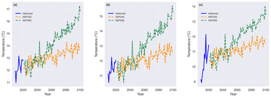
Figure 7.
Yearly average water temperature (°C) for (a) river, (b) lagoon, and (c) sea locations, based on historical observations (2009–2020) and projections (2021–2100) under SSP2-4.5 and SSP5-8.5 scenarios.
The historical water temperature data provide a reference for past trends, while the future projections under SSP2-4.5 and SSP5-8.5 depict possible temperature trajectories based on different greenhouse gas emission scenarios. The results indicate a steady warming trend across all three environments, with the rate and magnitude of warming varying between scenarios and water types. Across all environments, the SSP5-8.5 scenario—representing high greenhouse gas emissions and minimal mitigation efforts—shows the most pronounced increase in water temperature throughout the 21st century. Under this scenario, water temperatures are projected to rise substantially, reaching approximately 16–17 °C in the river (Figure 7a), 15–16 °C in the lagoon (Figure 7b), and around 14 °C in the sea (Figure 7c) by 2100. This rapid warming trend reflects the direct impact of increasing air temperature (as seen in Figure 6) and its influence on surface water heating. In contrast, the SSP2-4.5 scenario—characterized by moderate emissions reductions—shows a more gradual increase in water temperature. Although warming is still evident, the projected temperatures remain lower than those under SSP5-8.5, stabilizing around 13 °C in rivers, 12.5 °C in estuaries, and 12 °C in seas by the end of the century. This suggests that implementing climate mitigation policies could significantly reduce the extent of water temperature rise, potentially limiting the adverse effects on aquatic ecosystems. Among the three environments, sea water temperature (Figure 7c) exhibits the most stable trajectory with less variability, likely due to the ocean’s high thermal inertia, which moderates short-term fluctuations. In contrast, the river (Figure 7a) and lagoon (Figure 7b) temperatures display greater year-to-year variability, reflecting the influence of local hydrological conditions, seasonal variations, and interactions between land and water.
The projected trends in air temperature (Figure 6) and water temperature (Figure 7) indicate a strong correlation between atmospheric warming and aquatic thermal dynamics across river, lagoon, and sea environments from 2009 to 2100. The increases in water temperature closely follow the trends in air temperature under both SSP245 (moderate emissions scenario) and SSP5-8.5 (high emissions scenario), highlighting the direct influence of atmospheric warming on aquatic systems. Under SSP5-8.5, which represents a high greenhouse gas emissions trajectory, both air and water temperatures exhibit a significant upward trend throughout the 21st century. The warming in air temperature (Figure 6) leads to a corresponding rise in water temperature (Figure 7). According to the SSP245 and SSP5-8.5 scenario, the increase in air temperatures in the period of 2021–2100 could range from 1.5 to 1.7 °C and 4.7 to 5.1 °C, respectively. In contrast, the increase in water temperatures between 2021 and 2100 will be between 1.2 °C (for the sea) and 1.6 °C (for the river) under the SSP2-4.5 scenario and between 3.5 and 4.9 °C for the SSP5-8.5 scenario, respectively. Changes in water temperature according to the Mann–Kendall test in all water environments considering scenarios SSP2-4.5 and SSP5-8.5 are significant at the 0.05 level. This pronounced warming is particularly evident in river (Figure 7a) and lagoon (Figure 7b) environments, where air temperature variations exert stronger influences due to their lower thermal inertia and greater exposure to direct atmospheric heating. In contrast, the SSP2-4.5 scenario, which assumes moderate climate mitigation efforts, results in a lower but still noticeable increase in both air and water temperatures. The differences between SSP2-4.5 and SSP5-8.5 in both figures highlight the potential benefits of emissions reduction strategies in limiting future warming. The projected water temperature increases under SSP2-4.5 are more gradual and stabilize at lower values compared to those under SSP5-8.5, suggesting that climate policies aimed at reducing greenhouse gas emissions could help mitigate excessive warming in aquatic ecosystems. Among the three environments, sea water temperature (Figure 7c) exhibits the most stable trajectory, with the lowest variability over time. This pattern is consistent with the higher thermal inertia of the ocean, which allows it to absorb and store heat more effectively, moderating short-term fluctuations in temperature. In contrast, river and lagoon environments show greater variability of water temperatures (Figure 7a,b), reflecting their sensitivity to atmospheric changes and local hydrological conditions.
Table 4 presents a comparative summary of the linear regression slopes and projected end-of-century (year 2100) temperatures for both air and water across riverine, estuarine, and marine environments under the SSP2-4.5 and SSP5-8.5 climate scenarios.
Table 4.
Summary of linear regression slopes (°C/decade) and projected end-of-century temperatures (year 2100, in °C) for air and water temperatures across river, estuary, and sea environments under SSP2-4.5 and SSP5-8.5 scenarios. Air temperature values are based on Random Forest projections; water temperature trends are derived from statistically downscaled model outputs.
The scenario-based trends suggest potential differences in warming rates and absolute temperature values between scenarios, spatial domains, and media (air vs. water). Under the SSP2-4.5 scenario, the projected warming rates for air temperatures range from 0.19 to 0.22 °C per decade, while water temperatures increase at a slightly lower rate of 0.13 to 0.17 °C per decade. The highest air temperature in 2100 is projected for the riverine location (11.6 °C), while the warmest water temperature is observed in the same domain (14.0 °C). This pattern suggests a stronger sensitivity of inland water bodies to warming under moderate emissions, likely due to their limited thermal buffering capacity compared to larger coastal or marine systems. In contrast, the SSP5-8.5 scenario exhibits significantly accelerated warming across all domains. Air temperatures increase by 0.57 to 0.62 °C per decade, while water temperatures rise by 0.40 to 0.50 °C per decade. End-of-century air temperatures exceed 13.5 °C in sea and estuary environments, reaching 14.25 °C in the river system. Corresponding water temperatures are projected to reach as high as 16.7 °C in rivers and 15.5 °C in estuaries, reflecting intensified thermal responses under high-emission conditions.
4. Discussion
The study analyzed changes in surface water temperature across three different environments located in Central Europe. In each case, a correlation with air temperature was observed, confirming findings from previous studies on similar topics [59,60]. This relationship is crucial in the context of climate change and the ongoing increase in water temperature. Research conducted in Portugal (Coastal Lagoon Ria Formosa) showed that an air temperature increase of 1.68 °C leads to a water temperature rise of 0–1 °C [61]. The warming trend of average surface water temperatures in lagoons was found to be 0.03 °C per year between 1961 and 2008 [62]. In river estuaries of the Japanese archipelago, studies revealed a significant monthly increase in water temperature, with the highest recorded in October (0.090 °C per year) and the lowest in February (0.068 °C per year) [63]. Historical data confirm that water bodies are gradually warming. Świątek [64] found a statistically significant increase in the Baltic Sea’s water temperature at the Międzyzdroje station between 1950 and 2015. Similarly, for two stations on the Odra River, the average annual water temperature rose by 0.32 °C to 0.39 °C from 1965 to 2014 [65]. However, current research on projecting future water temperature changes remains insufficient, highlighting the need for further studies. This study demonstrates that the machine learning (ML) approach outperforms Bayesian Model Averaging (BMA) and statistical downscaling in predicting water temperature across river, lagoon, and sea environments. The superior performance of ML, particularly for sea temperature predictions, highlights its ability to capture complex, non-linear interactions between atmospheric and aquatic processes. In contrast, BMA and statistical downscaling, while improving resolution and reducing bias, are limited by their reliance on predefined statistical relationships, which may not fully represent dynamic climate patterns. The higher predictive accuracy for sea water temperature compared to river and lagoon temperatures can be attributed to the greater thermal inertia and stability of the ocean. Unlike rivers and estuaries, where temperature variations are more sensitive to short-term meteorological changes and freshwater inflows, the sea environment exhibits gradual, predictable fluctuations governed by large-scale climate processes such as ocean circulation, SST anomalies, and heat storage capacity [66]. The inclusion of SST-specific predictors significantly improves sea temperature forecasts, capturing large-scale climate oscillations and ocean–atmosphere feedbacks [67]. The incorporation of sea surface temperature (SST) data further enhances sea temperature predictions, as SST is a key driver of the ocean–atmosphere interactions that regulate energy fluxes and thermal gradients [68]. Furthermore, the research by Kowalewska-Kalkowska [69] indicates that the water temperature in the Pomeranian Bay is influenced by the water temperature of the Odra River (during high water levels), which reduces the impact of air temperature.
It is important to emphasize here that the article analyzes a station located in the coastal zone, not in the open sea. Coastal SST (Sea Surface Temperature) changes are greater than those of the global average and the open ocean [70]. Studies conducted in the northern English Channel have shown that the upward trend in SST is strongest in the coastal zone and decreases with distance from the shore [71]. In general, water thermal dynamics in coastal areas show a strong relationship with air temperature [59]. In the case of the coastal zone of the North Atlantic (St. Lawrence Gulf), SST shows a strong correlation with air temperature. These relationships are helpful in predicting the response of Gulf water temperatures to climate change [72]. In contrast, in the Szczecin Lagoon, its morphometry determines the close relationship between water temperature and air temperature [24]. It is a shallow water body, easily mixed to the bottom by wind. This results in minimal thermal variation and water that is nearly thermally uniform for most of the year [24].
Scenario-based projections under SSP2-4.5 (moderate emissions) and SSP5-8.5 (high emissions) suggest differential warming patterns across aquatic environments. Under SSP5-8.5, river and lagoon temperatures are expected to rise by 3–5 °C by 2100, whereas sea temperatures exhibit a relatively lower increase of 2–4 °C. These results are consistent with other studies, which also predict a several-degree increase in water temperature. According to projections, the water temperature in the Curonian Lagoon (southeastern part of the Baltic Sea) is expected to rise by 2–6 °C by 2100 [73]. The temperature of the Pilica River (central Poland) will increase by about 3 °C by the end of the 21st century [74]. In East Asia, studies have shown that sea surface temperature will rise by 4.5 °C under the SSP5-8.5 scenario, with the greatest increase occurring in the Yellow Sea, East China Sea, and East Sea [75].
Water temperature is a key element for other parameters and processes closely related to it. If the scenario-based projections are realized, an average increase of several degrees is expected over the next few decades. These results are concerning in the context of ecological status, which is currently poor (Odra River), weak (Szczecin Lagoon), and moderate (Pomeranian Bay, Baltic Sea) [76]. In the case of the Odra River, its ecological state is determined by total nitrogen, nitrate nitrogen, phytoplankton, macroinvertebrates, and ichthyofauna. For the Szczecin Lagoon, the above state is influenced by ammonium nitrogen, total phosphorus, phytoplankton, macroalgae, macroinvertebrates, and ichthyofauna. The moderate ecological state of Pomeranian Bay is determined by mineral nitrogen, total nitrogen, phytoplankton, and macroinvertebrates. Overall, the general water quality in all three cases has been rated as poor [76]. One of the main characteristics that determine water quality is the amount of dissolved oxygen, which, like all gases, is temperature-dependent. As Ptak and Nowak [77] report, oxygen levels are crucial for maintaining water quality, particularly in the context of ongoing eutrophication. Hypoxia is a common phenomenon affecting most parts of the lagoon. On average, the Szczecin Lagoon retains 253 tons of phosphorus and 17,278 tons of nitrogen influx per year [78]. Water temperature has a positive and strong influence on potential nutrient regeneration, and the intensity of thermal influence will gradually increase [79]. Any potential actions to improve water quality should therefore take into account the progressive rise in water temperature over the long term.
The mouth of the Odra River is one of the most vulnerable areas in the Baltic Sea to the immigration of alien species [80]. Even slight changes in temperature and salinity can affect the invasion patterns and dynamics of non-native species in the Baltic Sea [81]. Research by Zięba et al. [82] indicates that L. gibbosus currently poses an invasive risk in Poland, and this risk is likely to increase under future, warmer climate conditions. The simulated rise in water temperature at all three locations analyzed in the article will impact habitat conditions, and exceeding thermal thresholds for native flora and fauna may lead to their displacement by invasive species. Studies of European fish species in the coastal streams of the southern Baltic already show that species with an upper temperature tolerance threshold of <28 °C are living at the edge of their range in the studied region [83].
While the modeling framework demonstrates high performance during the calibration period (2009–2020), it is important to highlight a key limitation. The calibration window for the bias correction and statistical downscaling procedures spans only six years (2009–2014). This falls short of the standard 30-year climatological baseline typically required for robust climatological inference. The use of such a short window may lead to the overfitting of empirical distributions in the quantile mapping process and the reduced generalizability of derived statistical relationships. Consequently, the results presented here should be interpreted as a scenario-based modeling exercise grounded in short-term observations, rather than as a comprehensive climatological projection. Future work will seek to incorporate longer observational records to improve statistical stability and predictive robustness. It is also essential to recognize the increasing uncertainty associated with long-term projections extending to 2100. Such uncertainty arises from multiple sources, including unknown future emissions trajectories, socioeconomic developments, land-use changes, and possible non-linear feedbacks in the climate system. To address this, the study adopts an ensemble-based approach using Bayesian Model Averaging (BMA) with multiple CMIP6 global climate models, which helps to reduce structural model bias and capture a range of plausible futures. Furthermore, the use of standardized SSP2-4.5 and SSP5-8.5 scenarios enables a structured assessment of climate outcomes under varying emission pathways. Nonetheless, projections beyond several decades should be interpreted with caution, particularly regarding fine-scale variability, and should be viewed as scenario-based trends rather than deterministic forecasts. Uncertainties in future climate projections due to changing atmospheric circulation patterns and land-use modifications may affect model reliability under extreme climate scenarios [84]. Addressing these challenges requires continued model refinement, incorporating real-time climate data assimilation techniques and ensemble simulations to quantify uncertainty ranges [85]. Furthermore, in the analyzed cases, in addition to air temperature, the models should be expanded to include factors related to the delivery of thermal pollution and hydrological conditions associated with circulation and water exchange.
5. Conclusions
Water temperature is one of its fundamental characteristics, determining the course of processes and phenomena occurring within it. Currently, one of the main challenges in hydrosphere research is determining the thermal regime’s response to global warming, which relates to future changes. This study analyzes such responses for three aquatic environments: a river, a lagoon, and the sea in Central Europe. A multi-stage approach was used by integrating Bayesian regression averaging models (BMA), Random Sample Consensus regression (RANSAC), Gradient Boosting Regression (GBR), and a Random Forest machine learning model (RF). The results indicate that the RF method performs exceptionally well across all water types, with consistently high R2 values and low error metrics. The results show that by the end of the 21st century, scenario-based projections indicate a likely increase in water temperature across all cases. Changes in water temperature according to the Mann–Kendall test in all water environments considering scenarios SSP245 and SSP585 are significant at the 0.05 level. The extent of these changes depends on the adopted scenario, ranging from 1.2 °C for SSP2-4.5 to 1.6 °C, 3.5 °C, and 4.9 °C for SSP5-8.5. The estimated range of changes presents a challenge for the functioning of all three ecosystems, considering water quality and hydrobiological conditions. The simulated rise in water temperature under the modeled scenarios may impact habitat conditions, and exceeding thermal thresholds for native flora and fauna may lead to their displacement by invasive species.
Supplementary Materials
The following supporting information can be downloaded at: https://www.mdpi.com/article/10.3390/forecast7020024/s1, Figure S1. Leave-One-Year-Out Cross-Validation (LOYOCV) scatterplot of predicted vs. actual water temperature for the Sea environment. Each color represents a different validation year. Figure S2. LOYOCV performance metrics: R2, MAE, and RMSE values, by year for the Sea environment. Figure S3. Leave-One-Year-Out Cross-Validation (LOYOCV) scatterplot of predicted vs. actual water temperature for the lagoon environment. Each color represents a different. Figure S4. LOYOCV performance metrics: R2, MAE, and RMSE values, by year for the lagoon environment. Figure S5. Leave-One-Year-Out Cross-Validation (LOYOCV) scatterplot of predicted vs. actual water temperature for the river environment. Each color represents a different. Figure S6. LOYOCV performance metrics: R2, MAE, and RMSE values, by year for the river environment.
Author Contributions
Conceptualization, M.P.; methodology, T.A. and M.S.; software, T.A. and M.S. validation, T.A. and M.S.; formal analysis, T.A., M.P., and M.S., investigation, T.A., M.P., and M.S.; resources, M.P. and K.S.-P.; data curation, M.P. and K.S.-P.; writing—original draft preparation, M.P., T.A., M.S., and K.S.-P.; writing—review and editing, M.P., T.A., M.S., and K.S.-P.; visualization, M.P., T.A., and M.S.; supervision, M.P.; project administration, M.P.; funding acquisition, M.P. All authors have read and agreed to the published version of the manuscript.
Funding
This research received no external funding.
Data Availability Statement
Dataset available on request from the authors.
Conflicts of Interest
The authors declare no conflicts of interest.
References
- Choiński, A.; Ptak, M.; Strzelczak, A. Present-day evolution of coastal lakes based on the example of Jamno and Bukowo (the Southern Baltic coast). Oceanol. Hydrobiol. Stud. 2014, 43, 178–184. [Google Scholar] [CrossRef]
- Bintz, J.C.; Nixon, S.W.; Buckley, B.A.; Granger, S.L. Impacts of temperature and nutrients on coastal lagoon plant communities. Estuaries 2003, 26, 765–776. [Google Scholar] [CrossRef]
- Trombetta, T.; Bouget, F.Y.; Felix, C.; Mostajir, B.; Vidussi, F. Microbial diversity in a North Western Mediterranean Sea Shallow Coastal Lagoon under contrasting Water temperature conditions. Front. Mar. Sci. 2022, 9, 858744. [Google Scholar] [CrossRef]
- Dvoretsky, V.G.; Dvoretsky, A.G. Effects of water temperature on zooplankton abundance and biomass in the southwestern Barents Sea: Implications for Arctic monitoring and management. Ocean Coast. Manag. 2025, 261, 107506. [Google Scholar] [CrossRef]
- Lillis, A.; Mooney, T.A. Sounds of a changing sea: Temperature drives acoustic output by dominant biological sound-producers in shallow water habitats. Front. Mar. Sci. 2022, 9, 960881. [Google Scholar] [CrossRef]
- Ducharne, A. Importance of stream temperature to climate change impact on water quality. Hydrol. Earth Syst. Sci. 2008, 12, 797–810. [Google Scholar] [CrossRef]
- Kang, W.; Yang, X.; Jingqiao, M.; Yiqing, G.; Peipei, Z.; Gang, W. Study on the spawning period of typical fishes in the lower reaches of Jinsha River under the influence of water temperature change. J. Hohai Univ. 2023, 51, 50–55. [Google Scholar]
- Ptak, M.; Choiński, A.; Strzelczak, A.; Targosz, A. Disappearance of Lake Jelenino since the end of the XVIII century as an effect of anthropogenic transformations of the natural environment. Pol. J. Environ. Stud. 2013, 22, 191–196. [Google Scholar]
- Ptak, M.; Sojka, M.; Graf, R.; Choiński, A.; Zhu, S.; Nowak, B. Warming Vistula River—The effects of climate and local conditions on water temperature in one of the largest rivers in Europe. J. Hydrol. Hydromech. 2022, 70, 1–11. [Google Scholar] [CrossRef]
- Durance, I.; Ormerod, S.J. Trends in water quality and discharge confound long-term warming effects on river macroinvertebrates. Freshw. Boil. 2009, 54, 388–405. [Google Scholar] [CrossRef]
- Hausfather, Z.; Cowtan, K.; Clarke, D.C.; Jacobs, P.; Richardson, M.; Rohde, R. Assessing recent warming using instrumentally homogeneous sea surface temperature records. Sci. Adv. 2017, 3, e1601207. [Google Scholar] [CrossRef] [PubMed]
- Duan, H.; Yang, K.; Shang, C.; Zhou, X.; Luo, Y. Anthropogenic impact of lake surface water temperature of lakes: A case study of eleven lakes on the Yunnan-Guizhou Plateau. Ecol. Indic. 2024, 165, 112165. [Google Scholar] [CrossRef]
- Zannella, A.; Simonetti, I.; Lubello, C.; Cappietti, L. Hydrodynamics, transport time scales and water temperature dynamics in heavily anthropized eutrophic coastal lagoons, submitted for publication. Estuar. Coast. Shelf 2025, 314, 109146. [Google Scholar] [CrossRef]
- Zeighami, A.; Kurylyk, B.L. Modelled Water Temperature Patterns and Energy Balance of a Threatened Coastal Lagoon Ecosystem. Hydrol. Process. 2025, 39, e70068. [Google Scholar] [CrossRef]
- Stefan, H.G.; Sinokrot, B.A. Projected global climate change impact on water temperatures in five north central U.S. streams. Clim. Change 1993, 24, 353–381. [Google Scholar] [CrossRef]
- Khalil, I.; Atkinson, P.M.; Challenor, P. Looking back and looking forwards: Historical and future trends in sea surface temperature (SST) in the Indo–Pacific region from 1982 to 2100. Int. J. Appl. Earth Obs. Geoinf. 2016, 45, 14–26. [Google Scholar] [CrossRef]
- Mullin, C.A.; Kirchhoff, C.J.; Wang, G.; Vlahos, P. Future projections of water temperature and thermal stratification in Connecticut reservoirs and possible implications for cyanobacteria. Water Resour. Res. 2020, 56, e2020WR027185. [Google Scholar] [CrossRef]
- Ptak, M.; Amnuaylojaroen, T.; Sojka, M. Seven decades of surface temperature changes in central European lakes. What’s next? Resources 2024, 13, 149. [Google Scholar] [CrossRef]
- Ptak, M.; Amnuaylojaroen, T.; Sojka, M. Rivers increasingly warmer—Pediction of changes in the thermal regime of rivers in Poland. J. Geogr. Sci. 2025, 35, 139–172. [Google Scholar] [CrossRef]
- Tórz, A.; Nędzarek, A. The variability in concentrations of chosen nitrogen and phosphorus forms in the Oder River estuary in 1999–2002. Oceanol. Hydrobiol. Stud. 2010, 39, 113–120. [Google Scholar] [CrossRef]
- Dąbrowski, J.; Więcaszek, B.; Brysiewicz, A.; Czerniejewski, P. Which Fish Predators Can Tell Us the Most about Changes in the Ecosystem of the Pomeranian Bay in the Southwest Baltic Proper? Water 2024, 16, 2788. [Google Scholar] [CrossRef]
- Zwoliński, Z.; Kostrzewski, A.; Winowski, M.; Mazurek, M. Wolin Island—Outstanding geodiversity on the Polish Coast. In Landscapes and Landforms of Poland; Migoń, P., Jancewicz, K., Eds.; Springer: Cham, Switzerland, 2024; pp. 687–708. [Google Scholar]
- Wrzesiński, D. Entropia odpływu rzek w Polsce. In Studia i Prace z Geografii i Geologii; Bogucki Wydawnictwo Naukowe: Poznań, Poland, 2013; Volume 33. [Google Scholar]
- Majewski, A. Zalew Szczeciński; Wydawnictwa Komunikacji i Łączności: Warszawa, Poland, 1980. [Google Scholar]
- Osadczuk, A. Zalew Szczeciński- Środowiskowe Warunki Współczesnej Sedymentacji Lagunowej; Uniwersytet Szczeciński: Szczecin, Poland, 2004. [Google Scholar]
- Robak, S.; Zieliński, G.; Pańczyk, M.; Chmieliński, P.; Nermer, T. Skład i udział badanych pierwiastków chemicznych w otolicie węgorza europejskiego Anguilla anguilla (L.) pochodzącego z Zalewu Szczecińskiego. Komun. Rybackie 2018, 5, 1–5. [Google Scholar]
- Tomaszewski, J.B.; Tomaszewska, J. Charakterystyka fizjograficzna poszczególnych części estuarium. In Estuarium Odry i Zatoka Pomorska w Rozwoju Społeczno-Gospodarczym Polski; Uniwersytet Szczeciński: Szczecin, Poland, 1990. [Google Scholar]
- Seland, Ø.; Bentsen, M.; Olivié, D.; Toniazzo, T.; Gjermundsen, A.; Graff, L.S.; Debernard, J.B.; Gupta, A.K.; He, Y.C.; Kirkevåg, A.; et al. Overview of the Norwegian Earth System Model (NorESM2) and key climate response of CMIP6 DECK, historical, and scenario simulations. Geosci. Model Dev. 2020, 13, 6165–6200. [Google Scholar] [CrossRef]
- Müller, W.A.; Jungclaus, J.H.; Mauritsen, T.; Baehr, J.; Bittner, M.; Budich, R.; Bunzel, F.; Esch, M.; Ghosh, R.; Haak, H.; et al. A higher-resolution version of the Max Planck Institute Earth System Model (MPI-ESM1.2-HR). J. Adv. Model. Earth Syst. 2018, 10, 1383–1413. [Google Scholar] [CrossRef]
- Döscher, R.; Acosta, M.; Alessandri, A.; Anthoni, P.; Arneth, A.; Arsouze, T.; Bergmann, T.; Bernadello, R.; Bousetta, S.; Caron, L.P.; et al. The EC-Earth3 Earth system model for the Coupled Model Intercomparison Project 6. Geosci. Model Dev. 2022, 15, 2973–3020. [Google Scholar] [CrossRef]
- Semmler, T.; Danilov, S.; Gierz, P.; Goessling, H.F.; Hegewald, J.; Hinrichs, C.; Koldunov, N.; Khosravi, N.; Mu, L.; Rackow, T.; et al. Simulations for CMIP6 with the AWI climate model AWI-CM-1-1. J. Adv. Model. Earth Syst. 2020, 12, e2019MS002009. [Google Scholar] [CrossRef]
- Xin, X.-G.; Wu, T.-W.; Zhang, J.; Zhang, F.; Li, W.-P.; Zhang, Y.-W.; Lu, Y.-X.; Fang, Y.-J.; Jie, W.-H.; Zhang, L.; et al. Introduction of BCC models and its participation in CMIP6. Adv. Clim. Change Res. 2019, 15, 533. [Google Scholar]
- Yukimoto, S.; Kawai, H.; Koshiro, T.; Oshima, N.; Yoshida, K.; Urakawa, S.; Tsujino, H.; Deushi, M.; Tanaka, T.; Hosaka, M.; et al. The Meteorological Research Institute Earth System Model version 2.0, MRI-ESM2.0: Description and basic evaluation of the physical component. J. Meteorol. Soc. Jpn. Ser. II 2019, 97, 931–965. [Google Scholar] [CrossRef]
- Dunne, J.P.; Horowitz, L.W.; Adcroft, A.J.; Ginoux, P.; Held, I.M.; John, J.G.; Krasting, J.P.; Malyshev, S.; Naik, V.; Paulot, F.; et al. The GFDL Earth System Model version 4.1 (GFDL-ESM 4.1): Overall coupled model description and simulation characteristics. J. Adv. Model. Earth Syst. 2020, 12, e2019MS002015. [Google Scholar] [CrossRef]
- Lauritzen, P.H.; Nair, R.D.; Herrington, A.; Callaghan, P.; Goldhaber, S.; Dennis, J.; Bacmeister, J.; Eaton, B.; Zarzycki, C.; Taylor, M.A.; et al. NCAR release of CAM-SE in CESM2.0: A reformulation of the spectral element dynamical core in dry-mass vertical coordinates with comprehensive treatment of condensates and energy. J. Adv. Model. Earth Syst. 2018, 10, 1537–1570. [Google Scholar] [CrossRef]
- Cherchi, A.; Fogli, P.G.; Lovato, T.; Peano, D.; Iovino, D.; Gualdi, S.; Masina, S.; Scoccimarro, E.; Materia, S.; Bellucci, A.; et al. Global mean climate and main patterns of variability in the CMCC-CM2 coupled model. J. Adv. Model. Earth Syst. 2019, 11, 185–209. [Google Scholar] [CrossRef]
- Hoeting, J.A.; Madigan, D.; Raftery, A.E.; Volinsky, C.T. Bayesian model averaging: A tutorial (with comments by M. Clyde, David Draper and EI George, and a rejoinder by the authors. Stat. Sci. 1999, 14, 382–417. [Google Scholar] [CrossRef]
- Amnuaylojaroen, T. Advancements in Downscaling Global Climate Model Temperature Data in Southeast Asia: A Machine Learning Approach. Forecasting 2023, 6, 1–17. [Google Scholar] [CrossRef]
- Gudmundsson, L.; Bremnes, J.B.; Haugen, J.E.; Engen-Skaugen, T. Downscaling RCM precipitation to the station scale using statistical transformations–a comparison of methods. Hydrol. Earth Syst. Sci. 2023, 16, 3383–3390. [Google Scholar] [CrossRef]
- Maraun, D.; Wetterhall, F.; Ireson, A.M.; Chandler, R.E.; Kendon, E.J.; Widmann, M.; Brienen, S.; Rust, H.W.; Sauter, T.; Themeßl, M.; et al. Precipitation downscaling under climate change: Recent developments to bridge the gap between dynamical models and the end user. Rev. Geophys. 2010, 48, 3. [Google Scholar] [CrossRef]
- Rousseeuw, P.J. Robust Regression and Outlier Detection; John Wiley & Sons: Hoboken, NJ, USA, 1987. [Google Scholar]
- Schär, C.; Vidale, P.L.; Lüthi, D.; Frei, C.; Häberli, C.; Liniger, M.A.; Appenzeller, C. The role of increasing temperature variability in European summer heatwaves. Nature 2004, 427, 332–336. [Google Scholar] [CrossRef]
- Friedman, J.H. Greedy function approximation: A gradient boosting machine. Ann. Stat. 2001, 29, 1189–1232. [Google Scholar] [CrossRef]
- Hastie, T. The Elements of Statistical Learning: Data Mining, Inference, and Prediction; Taylor and Francis: New York, NY, USA, 2009. [Google Scholar]
- Chen, T.; Guestrin, C. Xgboost: A scalable tree boosting system. In Proceedings of the 22nd ACM Sigkdd International Conference on Knowledge Discovery and Data Mining, San Francisco, CA, USA, 13–17 August 2016; pp. 785–794. [Google Scholar]
- Breiman, L. Random forests. Mach. Learn. 2001, 45, 5–32. [Google Scholar] [CrossRef]
- Huang, B.; Liu, C.; Banzon, V.; Freeman, E.; Graham, G.; Hankins, B.; Smith, T.; Zhang, H.-M. Improvements of the Daily Optimum Interpolation Sea Surface Temperature (DOISST) Version 2.1. J. Clim. 2021, 34, 2923–2939. [Google Scholar] [CrossRef]
- Reynolds, R.W.; Smith, T.M.; Liu, C.; Chelton, D.B.; Casey, K.S.; Schlax, M.G. Daily High-Resolution-Blended Analyses for Sea Surface Temperature. J. Clim. 2007, 20, 5473–5496. [Google Scholar] [CrossRef]
- Haghbin, M.; Sharafati, A.; Motta, D.; Al-Ansari, N.; Noghani, M.H.M. Applications of soft computing models for predicting sea surface temperature: A comprehensive review and assessment. Prog. Earth Planet. Sci. 2021, 8, 4. [Google Scholar] [CrossRef]
- Miao, Y.; Zhang, C.; Zhang, X.; Zhang, L. A Multivariable Convolutional Neural Network for Forecasting Synoptic-Scale Sea Surface Temperature Anomalies in the South China Sea. Weather Forecast. 2023, 38, 849–863. [Google Scholar] [CrossRef]
- Fanelli, C.; Ciani, D.; Pisano, A.; Nardelli, B.B. Deep learning for the super resolution of Mediterranean sea surface temperature fields. Ocean Sci. 2024, 20, 1035–1050. [Google Scholar] [CrossRef]
- Hirons, L.C.; Klingaman, N.P.; Woolnough, S.J. The impact of air-sea interactions on the representation of tropical precipitation extremes. J. Adv. Model. Earth Syst. 2018, 10, 550–559. [Google Scholar] [CrossRef]
- Kendall, M.G.; Stuart, A. The Advanced Theory of Statistics, 3rd ed.; Charles Griffin Ltd.: Cheshire, UK, 1968. [Google Scholar]
- Gilbert, R.O. Statistical Methods for Environmental Pollution Monitorin; Van Nostrand Reinhold Co.: New York, NY, USA, 1987. [Google Scholar]
- Patakamuri, S.K.; O’Brien, N. Modified Versions of Mann Kendall and Spearman’s Rho Trend Tests, Version 1.6; Water Resources Publication: Littleton, CO, USA, 2022.
- Probst, P.; Wright, M.N.; Boulesteix, A.L. Hyperparameters and tuning strategies for random forest. Wiley Interdiscip. Rev. Data Min. Knowl. Discov. 2019, 9, e1301. [Google Scholar] [CrossRef]
- James, G.; Witten, D.; Hastie, T.; Tibshirani, R. An Introduction to Statistical Learning with Applications in R; Springer: New York, NY, USA, 2013. [Google Scholar]
- Cutler, D.R.; Edwards, T.C.; Beard, K.H.; Cutler, A.; Hess, K.T.; Gibson, J.; Lawler, J.J. Random Forests for Classification in Ecology. Ecology 2012, 88, 2783–2792. [Google Scholar] [CrossRef]
- Zhu, S.; Luo, Y.; Ptak, M.; Sojka, M.; Ji, Q.; Choiński, A.; Kuang, M. A hybrid model for the forecasting of sea surface water temperature using the information of air temperature: A case study of the Baltic Sea. All Earth 2022, 34, 27–38. [Google Scholar] [CrossRef]
- Ptak, M.; Sojka, M.; Nowak, B. Effect of climate warming on a change in thermal and ice conditions in the largest lake in Poland—Lake Śniardwy. J. Hydrol. Hydrodyn. 2020, 68, 260–270. [Google Scholar] [CrossRef]
- Rodrigues, M.; Rosa, A.; Cravo, A.; Jacob, J.; Fortunato, A.B. Effects of Climate Change and Anthropogenic Pressures in the Water Quality of a Coastal Lagoon (Ria Formosa, Portugal). Sci. Total Environ. 2021, 780, 146311. [Google Scholar] [CrossRef]
- Dailidienė, I.; Baudler, H.; Chubarenko, B.; Navrotskaya, S. Long term water level and surface temperature changes in the lagoons of the southern and eastern Baltic. Oceanologia 2011, 53, 293–308. [Google Scholar] [CrossRef]
- Itsukushima, R.; Ohtsuki, K.; Sato, T. Drivers of rising monthly water temperature in river estuaries. Limnol. Oceanogr. 2024, 69, 589–603. [Google Scholar] [CrossRef]
- Świątek, M. Long-term variability of water temperature and salinity at the Polish coast. Bull. Geogr. Phys. Geogr. Ser. 2019, 16, 115–130. [Google Scholar] [CrossRef]
- Choiński, A.; Ptak, M.; Volchak, A.; Kirvel, I.; Valiuškevičius, G.; Parfomuk, S.; Kirvel, P.; Sidak, S. Effect of Air Temperature Increase on Changes in Thermal Regime of the Oder and Neman Rivers Flowing into the Baltic Sea. Atmosphere 2021, 12, 498. [Google Scholar] [CrossRef]
- Henson, S.A.; Beaulieu, C.; Ilyina, T.; John, J.G.; Long, M.; Séférian, R.; Tjiputra, J.; Sarmiento, J.L. Rapid emergence of climate change in environmental drivers of marine ecosystems. Nat. Commun. 2017, 8, 14682. [Google Scholar] [CrossRef] [PubMed]
- Siqueira, L.; Kirtman, B.P. Atlantic near-term climate variability and the role of a resolved Gulf Stream. Geophys. Res. Lett. 2016, 43, 3964–3972. [Google Scholar] [CrossRef]
- Chelton, D.B.; Schlax, M.G.; Freilich, M.H.; Milliff, R.F. Satellite measurements reveal persistent small-scale features in ocean winds. Science 2004, 303, 978–983. [Google Scholar] [CrossRef]
- Kowalewska-Kalkowska, H. Meteorological and hydrological determination of water temperature in the coastal area of the Pomeranian Bay. Balt. Coast. Zone 2000, 4, 15–26. [Google Scholar]
- Liao, E.; Lu, W.; Yan, X.H.; Jiang, Y.; Kidwell, A. The coastal ocean response to the global warming acceleration and hiatus. Sci. Rep. 2015, 5, 16630. [Google Scholar] [CrossRef]
- Kassem, H.; Amos, C.L.; Thompson, C.E.L. Sea surface temperature trends in the coastal zone of southern England. J. Coast. Res. 2023, 39, 18–31. [Google Scholar] [CrossRef]
- Galbraith, P.S.; Larouche, P.; Chassé, J.; Petrie, B. Sea-surface temperature in relation to air temperature in the Gulf of St. Lawrence: Interdecadal variability and long term trends. Deep-Sea Res. Part II Top. Stud. Oceanogr. 2012, 77–80, 10–20. [Google Scholar] [CrossRef]
- Jakimavičius, D.; Kriaučiūnienė, J.; Šarauskienė, D. Impact of climate change on the Curonian Lagoon water balance components, salinity and water temperature in the 21st century. Oceanologia 2018, 60, 378–389. [Google Scholar] [CrossRef]
- Ptak, M.; Amnuaylojaroen, T.; Sojka, M. Historical and future changes in water temperature of the Pilica River (Central Europe) in response to global warming. Sustainability 2024, 16, 10244. [Google Scholar] [CrossRef]
- Jung, H.; Jung, E.; Jang, C.J. Future changes in sea surface temperature in the East Asian Marginal Seas projected by CMIP6 models. Korea Soc. Coast. Disaster Prev. 2024, 11, 123–131. [Google Scholar] [CrossRef]
- Available online: www.hydroportal.pl (accessed on 20 February 2025).
- Ptak, M.; Nowak, B. Variability of oxygen-thermal conditions in selected lakes in Poland. Ecol. Chem. Eng. S 2016, 23, 639–650. [Google Scholar] [CrossRef]
- Neumann, T.; Schernewski, G.; Friedland, R. Transformation Processes in the Oder Lagoon as seen from a Model Perspective. EGUsphere 2025. preprint egusphere-2024-3734. [Google Scholar] [CrossRef]
- Kang, Y.; Lee, D.H. Coastal Warming Heightens Direct Impacts of Seawater Temperature on Nutrients near Aquaculture Farms in Korea. Sci. Total Environ. 2023, 892, 164643. [Google Scholar] [CrossRef]
- Gruszka, P. The River Odra estuary as a gateway for alien species immigration to the Baltic Sea basin. Acta Hydrochim. Hydrobiol. 1999, 27, 374–382. [Google Scholar] [CrossRef]
- Leppäkoski, E.; Gollasch, S.; Gruszka, P.; Ojaveer, H.; Olenin, S.; Panov, V. The Baltic—A sea of invaders. Can. J. Fish. Aquat. Sci. 2002, 59, 1175–1188. [Google Scholar] [CrossRef]
- Zięba, G.; Vilizzi, L.; Copp, G.H. How likely is Lepomis gibbosus to become invasive in Poland under conditions of climate warming? Acta Ichthyol. Piscat. 2020, 50, 35–51. [Google Scholar] [CrossRef]
- Radtke, G.; Bernaś, R. Temperature tolerance of European fish species based on thermal maxima in southern Baltic Sea-basin streams. Ecol. Indic. 2025, 170, 113107. [Google Scholar] [CrossRef]
- Stanzel, P.; Harald, K. From ENSEMBLES to CORDEX: Evolving climate change projections for Upper Danube River flow. J. Hydrol. 2018, 563, 987–999. [Google Scholar] [CrossRef]
- Pappenberger, F.; Dutra, E.; Wetterhall, F.; Cloke, H.L. Deriving global flood hazard maps of fluvial floods through a physical model cascade. Hydrol. Earth Syst. Sci. 2012, 16, 4143–4156. [Google Scholar] [CrossRef]
Disclaimer/Publisher’s Note: The statements, opinions and data contained in all publications are solely those of the individual author(s) and contributor(s) and not of MDPI and/or the editor(s). MDPI and/or the editor(s) disclaim responsibility for any injury to people or property resulting from any ideas, methods, instructions or products referred to in the content. |
© 2025 by the authors. Licensee MDPI, Basel, Switzerland. This article is an open access article distributed under the terms and conditions of the Creative Commons Attribution (CC BY) license (https://creativecommons.org/licenses/by/4.0/).