Abstract
This article describes a robust Gaussian Prior process state space modeling (GPSSM) approach to assess the impact of an intervention in a time series. Numerous applications can benefit from this approach. Examples include: (1) time series could be the stock price of a company and the intervention could be the acquisition of another company; (2) the time series under concern could be the noise coming out of an engine, and the intervention could be a corrective step taken to reduce the noise; (3) the time series could be the number of visits to a web service, and the intervention is changes done to the user interface; and so on. The approach we describe in this article applies to any times series and intervention combination. It is well known that Gaussian process (GP) prior models provide flexibility by placing a non-parametric prior on the functional form of the model. While GPSSMs enable us to model a time series in a state space framework by placing a Gaussian Process (GP) prior over the state transition function, probabilistic recurrent state space models (PRSSM) employ variational approximations for handling complicated posterior distributions in GPSSMs. The robust PRSSMs (R-PRSSMs) discussed in this article assume a scale mixture of normal distributions instead of the usually proposed normal distribution. This assumption will accommodate heavy-tailed behavior or anomalous observations in the time series. On any exogenous intervention, we use R-PRSSM for Bayesian fitting and forecasting of the IoT time series. By comparing forecasts with the future internal temperature observations, we can assess with a high level of confidence the impact of an intervention. The techniques presented in this paper are very generic and apply to any time series and intervention combination. To illustrate our techniques clearly, we employ a concrete example. The time series of interest will be an Internet of Things (IoT) stream of internal temperatures measured by an insurance firm to address the risk of pipe-freeze hazard in a building. We treat the pipe-freeze hazard alert as an exogenous intervention. A comparison of forecasts and the future observed temperatures will be utilized to assess whether an alerted customer took preventive action to prevent pipe-freeze loss.
1. Introduction
This paper deals with the problem of assessing the impact of an intervention in a time series. Specifically, we provide a robust Gaussian Prior process state space modeling (GPSSM) approach to solve this problem. There are numerous applications that could benefit from such approaches. A class of applications arises in the context of Internet of Things (IoTs). IoT describes interconnected physical sensors that communicate via the internet. In recent times, IoT technology exists in several domains. These include but are not limited to smart city energy consumption forecasting [1], sewer overflow monitoring [2], and development of risk mitigation strategies in the insurance industry [3,4]. This article focuses on the last application in the insurance industry, where IoT devices typically record their observations in a streaming fashion, leading to an inherent temporal dimension in the IoT datasets. Development of statistical and machine learning models for IoT data streams has two primary challenges. First, time series recorded by IoT devices are often characterized by complex temporal dependencies including non-linear dynamics, heavy-tailed behavior, anomalies, etc. Second, datasets on IoT time series can be massive, possibly consisting of thousands of sensors recording observations at high frequency (e.g., at 15 min intervals). Unfortunately, many traditional time series methods either do not scale easily to handle the size of such datasets or cannot adequately accommodate the complex temporal dynamics. There is a need to develop novel time series methods that are simultaneously flexible enough to learn the nuanced behavior of IoT time series and are also computationally feasible to potentially handle thousands of time series.
One application for sensor networks is temperature monitoring within buildings owned by end customers of an insurance firm. These buildings are susceptible to pipe-freeze hazard (freeze loss), and the explicit goal is to prevent pipe-freeze losses to the end customers through real-time alerts. A large number of sensors are usually deployed in buildings throughout the United States, and it is essential to automate the process of detecting and addressing adverse events (pipe-freeze loss). Critical to this process is anomaly detection in the temperature readings that are acquired from the sensors. Ref. [4] developed a modified Isolation Forest (IF+) machine learning algorithm to address pipe-freeze loss mitigation, which proved to be extremely useful in detecting anomalies in the temperature streams, which the firm used as the basis for sending customer alerts. Then, an important question is whether and how an alerted end customer (insured) took remedial action to prevent pipe freeze. Since direct feedback from the end customer on this is rarely available, an interesting though challenging alternative is to use patterns in the pre-alert and post-alert temperature streams to infer customer action.
A natural way to infer whether a customer took meaningful action after an alert is to develop a metric that assesses differences in pre-alert and post-alert behavior in the temperature streams by using time series intervention impact methods. In the classical (frequentist) framework, intervention analysis such as the methods proposed in [5,6] or change point detection [7] may be used for detecting whether there was a significant post-event change in the stochastic behavior of a time series. [8] described an intervention impact approach in the Bayesian framework by (a) employing a Bayesian structural time series (BSTS) model [9] to fit the pre-intervention time series, and (b) using forecasts from the fitted model to develop counter-factual forecasts of the post-intervention series. The difference between the observed post-intervention and the forecast post-intervention values of the time series allows one to construct a semi-parametric posterior estimate of the impact effect associated with the exogenous intervention. Unfortunately, the BSTS approach does not produce accurate results when the temporal dependence in the IoT streams is nonlinear.
Gaussian process (GP) prior models (or GP models, for short) describe a set of methods which generalize the multivariate normal to infinite dimensions. Gaussian process regression models [10] have also been extended to time series. In particular, this model offers an alternative to the Bayesian structural time series model for intervention impact assessment in time series; it provides greater flexibility by allowing us to place a non-parametric prior on the functional form of the model. The class of GP regression models has demonstrated excellent performance for time series forecasting tasks [11,12] by directly learning the functional form of the data through either maximum likelihood (ML), maximum a posteriori (MAP), or fully Bayesian procedures [13,14,15].
We employ the Gaussian process model framework to assess the intervention impact of customer action in the context of a long IoT time series of internal temperatures recorded by sensors. Specifically, by treating the pipe-freeze hazard alert as an exogenous intervention, we can assess whether we believe with a high level of confidence that an alerted customer took preventive action to prevent pipe-freeze loss.
Section 2 first reviews Gaussian state space models. Section 3 describes the robust Gaussian process state space models for forecasting time series. Section 4 describes how we can forecast IoT time series of internal temperatures using robust Gaussian process state space models, then assess the impact of customer reaction to an intervention (alert of pipe freeze hazard). Section 5 presents a summary and discussion.
2. Review of Variants of Gaussian Process State Space Models
Gaussian Process (GP) models have flexible non-parametric forms, and for supervised learning problems, they have the distinct advantage of allowing the user to automatically learn the correct functional form linking the input space to the output time series . This is achieved by specifying a prior over the distribution of functions, which then allows the derivation of the posterior distribution over these functions once the data have been observed. Through their flexibility and versatility, GP regression models have demonstrated excellent performance for regression tasks by directly learning the functional form of the data [10]. A review of GP regression and sparse GP regression models for time series is given in Appendix A.
Given a time series observed at discrete times , a state space model (SSM) assumes that the temporal dynamics in are governed by the history of an unobserved latent state vector , which evolves over time in a Markovian way [16]:
Equation (1) is the observation equation and (2) is the state equation. The function is a possibly nonlinear function relating the observed to , while is a possibly nonlinear state transition function which relates the current state to past values . In (1) and (2), and represent the observation and state errors, respectively. In many practical situations, we also have exogenous predictors , which may be included either in the state equation or the observation equation for explaining and predicting . In monitoring pipe-freeze hazard, can denote the internal temperature in a building at time t, and the exogenous predictor can be the vector .
The general form for the SSM in (1) and (2) includes linear SSMs such as the dynamic linear model (DLM) estimated via Kalman filtering [17], Bayesian structural time series (BSTS) models estimated via exact and approximate Bayesian methods [9,18], and models governed by nonlinear dynamics such as variants of Gaussian Process state space models, which we describe in this paper.
Section 2.1 gives the an overview of the current literature on the Gaussian Process state space model (GPSSM) [19]. Section 2.2 describes the probabilistic recurrent state space model (PRSSM) [20], which is a variant of the GPSSM.
2.1. Review of Gaussian Process State Space Models
A Gaussian Process state space model (GPSSM) is defined by placing a Gaussian Process (GP) prior over the state transition function in (2), yielding the following generative model:
where
denote the mean function and the covariance kernel, respectively, with the hyperparameter set denoted as , and is an arbitrary parametric density. Placing the GP prior over the state transition function endows the model with the ability to learn a wide array of non-linear transition behaviors from the data based on the structure of the kernel . A few examples of commonly used kernels in a time series context are shown in Appendix A. Note that while we have assumed a univariate response and univariate latent state (suitable for HSB’s IoT streams), the GPSSM can be easily extended to handle multivariate observations and latent states; further, the conditional distribution of can be assumed to depend on a larger set of hyperparameters instead of just the variance .
Let , , and , where . The joint p.d.f. for the generic GPSSM takes the following form:
where denotes the set of hyper-parameters. Under the assumed GP prior in a GPSSM, computing the joint posterior distribution is challenging due to the non-linear state transition function. Several exact and approximate Bayesian approaches have been proposed in the literature for state estimation and hyperparameter learning. Ref. [21] proposed an analytic moment-based filter for modeling non-linear stochastic dynamical systems with GPs by exploiting the Gaussian assumption in the filter step. Ref. [22] proposed using the expectation-maximization (EM) algorithm to perform inference in the the latent space and learn the parameters of the underlying GP dynamical model. Ref. [23] developed a variational inference approach (see [24]) for estimating the GPSSM by leveraging sparse Gaussian processes in conjunction with sequential Monte Carlo methods. To improve learning of the latent states in a GPSSM, ref. [25] proposed the use of a recurrent neural network to help recover the parameters of the variational approximation for the latent states. More recently, ref. [26] employed a non-factorized variational density that allows for direct modeling of the dependency between latent states and the GP posterior, thus improving the predictive performance of the model.
One notable variant of the GPSSM is the probabilistic recurrent state space model (PRSSM) introduced by [20]. This framework leverages variational inference and sparse GP methods to reduce computational complexity. More details on this model are given in Section 2.2.
2.2. Review of Probabilistic Recurrent State Space Models
Ref. [20] discussed the probabilistic recurrent state space model (PRSSM), which uses a specialized variational approximation capable of modeling temporal correlations among the latent states by coupling samples from the inducing variables to the latent states. PRSSM also employs a sparse inducing point GP approach to reduce computational complexity during estimation.
As defined earlier, let be the observed response time series vector, be the unobserved vector of latent states, and . Here, is assumed to be a multivariate Gaussian with mean vector and variance–covariance matrix . Let denote a small number of inducing points, let be inducing inputs, and let be the corresponding inducing variables.
The joint density of , and under the PRSSM has the following form:
where the details of the components on the right are given in [20]. The joint posterior is then approximated with the following joint variational density:
where denotes the variational density for the initial state, while is the variational density for the inducing variables. Estimation of the variational parameters in (8) is done by minimizing the evidence lower bound (ELBO), which has the following form:
One key advantage of this variational approximation is its preservation of correlations between time steps. This allows for optimization of the ELBO to remain tractable. One shortcoming of PRSSM is that it uses a Gaussian density for the observational equation, which may not be suitable for practical situations where there is heavy-tailed observational noise. In the next section, we propose replacing the Gaussian observation density with the p.d.f. of a scale mixture of Gaussians.
3. Robust Gaussian State Space Model
In many practical problems with heavy-tailed observational noise or anomalous data, the Gaussian likelihood for employed in the GPSSM or PRSSM may be inadequate for accurate forecasting because the probability distribution of the time series (here, the IoT temperatures) exhibits heavy-tailed behavior due to the presence of several outliers, for example. A remedy is to incorporate heavy-tailed non-Gaussian distribution in a model step. Ref. [27] described sparse latent autoregressive Student-t process models (TP-RLARX) (see Appendix A for details) by assuming the Student-t prior process for . The computational burden for estimation and forecasting for the TP-RLARX models can be high, and the model is not set up in a conventional SSM framework. In this section, we describe an alternative R-PRSSM approach.
To model and forecast a time series exhibiting heavy tails or outlier behavior (the IoT temperature series), we replace the normal distribution in PRSSM by a scale mixture of normals distribution [28] while retaining the Gaussian distribution . We refer to the corresponding model as the robust PRSSM or R-PRSSM. Recall that the scale mixture of normals distribution is defined as follows:
where is the variance of the normal distribution, so that
When is the inverse-Gamma density, (10) is the Student-t density, while if is the exponential density, then (10) is the Laplace density. Both of these distributions accommodate non-Gaussian behavior such as heavy tails or outliers.
Using notation similar to Section 2.2, we see that
where are inducing points. Based on the properties of the multivariate normal distribution [29], we see that
The joint density of , and under R-PRSSM with a Gaussian scale mixture distributional assumption is as follows:
where
and
are the GP predictive mean and covariance, as the conditional mean and covariance are defined in (12). Note that the conditional distribution in (12) only requires inversion of the matrix instead of the matrix . By setting , the computational burden is substantially reduced.
For fitting and forecasting via R-PRSSM, the target is the n-dimensional marginal distribution of , i.e.,
where the terms in the integral were shown in (12) and (13), respectively. Replacing with its variational approximation (see Appendix B for a review)
leads to approximating via a variational approximation , which has the following form (again using the properties of the multivariate normal distribution):
Incorporating the scale prior implies that the joint variational density becomes as follows:
where , denotes the variational density for the initial state, while is the variational density for the inducing variables. We employ an LSTM [30] recognition model to learn the initial latent state; more details can be found in [25].
The evidence lower bound (ELBO) for R-PRSSM takes the following form:
where is the Kullback–Leibler distance between and . In (20), the last two KL terms are analytically tractable and are given as follows:
and
where denotes the trace of a matrix . The term can be derived as follows:
The ELBO for the R-PRSSM is optimized using virtually the same stochastic variational inference procedure described in the original PRSSM paper by [20]. The only difference is that we have the following:
as the unbiased estimator for the log-likelihood, where s denotes the s-th sample from and .
The generic steps for forward and backward passes for the R-PRSSM variational inference algorithm are described in Algorithms 1 and 2. Below, we show the steps for implementing R-PRSSM for the internal temperature series . The inputs are the internal and ambient temperatures for time points for the training data and time points for the test data.
Our implementation of this algorithm for the IoT temperature time series is done using PyTorch [31] and GPyTorch [32]. These platforms include implementations for many state-of-the-art GP methods.
- Step 1. We initialize the variational parameters.
- Step 2. Using current variational parameters, we generate the n-dimensional latent state trajectories by sampling from multivariate Gaussian , and we sample from .
- Step 3. We evaluate the ELBO in (20) at the current values of the variational parameters and the generated samples in Step 2.
- Step 4. We update the variational parameters via a backward pass of the gradient descent algorithm using the *autodiff routine* in PyTorch.
We repeat these steps until the ELBO has attained convergence.
4. Application: Intervention Impact Analysis for IoT Temperature Time Series
We illustrate the approach for a data stream from a single sensor installed in a building by The Hartford Steam Boiler. Figure 1 shows the internal temperatures (blue) and the external temperatures (yellow) for the entire week prior to an alert event (vertical black line), as well as the observed values over the immediate twelve hours following the alert. That is, the training data length is (i.e., 15 min observations for a week), and the test data length is (i.e., 15 min observations for 12 h).
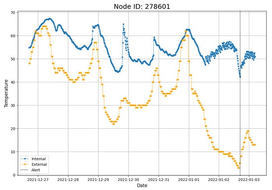
Figure 1.
Example Alert Event during a single week: the blue line is the internal temperature observed once every 15 min, the orange line is the external (ambient) temperature at the same times, and the dotted line is the time point of the alert.
In the hours immediately preceding the alert event, there is a precipitous decline in external temperatures along with sufficiently low internal temperatures, which together trigger an alert. Our code is a modified version of the code available here: https://github.com/zhidilin/gpssmProj/blob/main/models/GPSSMs.py, accessed on 23 May 2025, which was implemented as part of [33]. This repo has an implementation for PRSSM (see line 77, and set LMC = False on line 87).
We fit the R-PRSSM with a scale mixture of normal errors and a Mateŕn 52 kernel to the week-long internal temperatures prior to an alert event and forecast the next twelve hours ( time steps) post-alert. Note that we chose the Mateŕn 52 kernel, as it gave the best overall performance when compared to an RBF, Mateŕn 12 and Mateŕn 32 kernels. We compare the performance of R-PRSSM and PRSSM using the following prediction metrics: mean squared error (RMSE), mean absolute error (MAE), symmetric mean absolute percent error (SMAPE), and continuous ranked probability score (CRPS) [34].
The SMAPE for the test data is defined as follows:
It is designed to address the issue of negative errors being more heavily penalized by the standard MAPE calculation. The CRPS measures the quality of a probabilistic forecast and is defined as follows:
where F denotes the cumulative distribution function for the continuous random variable x, and denotes the indicator function. In Bayesian forecasting settings, the CRPS can be estimated by comparing the empirical CDF of the posterior predictive samples and the CDF of our observed values.
Since we are specifically interested in identifying anomalously large increases in the observed post-alert temperatures, we compute and compare the widths of the predictive intervals generated by the models. To do this, we use the prediction interval coverage probability (PICP), defined as follows:
where is the q-th quantile of the posterior predictive density of at time t. If the predictive interval is too narrow, it is likely that the intervention impact analysis is prone to false positives.
Figure 2 shows the 48-step-ahead (12 h) forecasts generated by the PRSSM (left) and the R-PRSSM (right). From the figure, we can see that both models are successful in learning the post-alert internal temperature dynamics, as evidenced by the posterior mean predictions. In addition, it is clear that the 95% posterior predictive interval from the PRSSM has failed to encompass a significant proportion of time points at both the start and end of the forecast period. In contrast, R-PRSSM’s 95% predictive interval fully encompasses the vast majority of the observed post-alert temperature readings.
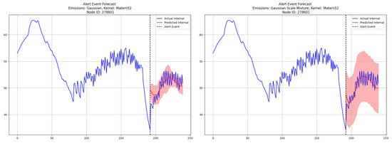
Figure 2.
Comparison forecasts post-alert for time points from the PRSSM model (left) and the R-PRSSM model (right). The post-alert period is the same as in Figure 1. We show a truncated pre-alert period for clarity.
A comparison of the forecast metrics for both models is given in Table 1 below. We observe that while the PRSSM mildly outperforms the R-PRSSM on metrics related to point prediction (RMSE, SMAPE, CRPS), it performs substantially worse than the R-PRSSM on the PICP metric. Since the predictive density for the PRSSM does not adequately capture the variance in the post-alert temperatures, subsequent intervention analysis is not reliable.

Table 1.
48-step-ahead forecast metrics comparison for the alert event shown in Figure 1.
The intervention impact p-value for the PRSSM is about 0.759, compared with a value of about 0.370 for the R-PRSSM. If the intervention impact p-value is greater than , we declared “action taken” on an alert event. While neither model would have classified this event as having appreciable customer intervention based on that criterion, we nevertheless see that the forecasts generated by the PRSSM model have a propensity to overestimate the likelihood of customer action due to its underestimation of the internal temperature variability. If the goal is to be more conservative in labeling alert events as receiving appreciable customer response, then the R-PRSSM with its heavier-tailed posterior predictive density should be preferred.
Having demonstrated the efficacy of this method on a single sensor, we apply both the PRSSM and the R-PRSSM methods to 50 sensor time series, each with a single alert. Overall, we find that while R-PRSSM performs worse on forecast metrics related to point prediction, as shown by the results in Table 2, it greatly outperforms PRSSM on the PICP metric. Furthermore, Table 3a,b show that the R-PRSSM is far more conservative in declaring an appreciable post-alert intervention (as indicated by a rise in temperature) by the customer, i.e., 16% of alerts under the R-PRSSM versus 28% under the PRSSM. Overall, if the goal of the firm is to be conservative in assessing customers as low-risk clients based on their propensity to react to alerts, then the R-PRSSM is the preferable method (since it provides wider predictive intervals).
Table 2.
48-Step-ahead forecast metrics comparison (averaged across 50 unique alert events from different IoT sensors).
Table 3.
Confusion matrices for PRSSM (a) and R-PRSSM (b) for analyzed alert events from the 50 sensors.
5. Summary and Discussion
In this paper, we proposed the R-PRSSM, which extends the Gaussian process state space model known as PRSSM by replacing the Gaussian likelihood with a Gaussian scale mixture likelihood. Our primary motivation in doing this was to make the PRSSM more robust to observational noise, then use it as the forecasting model for time series intervention analysis.
As a proof of concept, we applied the R-PRSSM to 50 IoT time series alert events and compared its performance with the PRSSM. We found that the R-PRSSM’s (additional) inverse Gamma prior for the scale parameter modifying the Gaussian likelihood led to improved predictive interval coverage probability compared to the PRSSM. As a result of its wider predictive intervals, the R-PRSSM’s intervention impact assessment was far more conservative than the corresponding assessment from the PRSSM. Indeed, if domain experts believe that the cost of false positives is high, then it would be prudent for them to use the R-PRSSM, since its intervention impact inference will be more robust to outliers and heavy-tailed noise distribution in the post-alert forecast period. We also mention that it is important to pay attention to model selection, hyperparameter tuning, and scalability. In addition, modeling choices, such as the use of a particular heavy-tailed likelihood, are important.
The results presented in this paper point to a number of fruitful avenues for future research. First, for simplicity, we presented a simple version of the PRSSM in which both the observations and latent state were univariate. However, the original paper by [20] is more general in that it allows for multivariate latent states and likelihoods. R-PRSSM could easily be extended to accommodate multivariate states and likelihoods by replacing the inverse Gamma prior with that of an inverse Wishart prior. Furthermore, we could also investigate whether or not anything would be gained by replacing the GP transition function with that of a TP, similar to the TPRLARX model from [27]. Finally, while we opted for the Gaussian scale mixture likelihood, other options such as the Laplace likelihood could also be explored.
Author Contributions
Conceptualization, P.T., N.R., N.L. and S.R.; methodology, P.T., N.R., N.L. and S.R.; software, P.T., N.R., N.L. and S.R.; validation, P.T., N.R., N.L. and S.R.; formal analysis, P.T., N.R., N.L. and S.R.; investigation, P.T., N.R., N.L. and S.R.; resources, P.T., N.R., N.L. and S.R.; data curation, P.T., N.R., N.L. and S.R.; writing—original draft preparation, P.T., N.R., N.L. and S.R.; writing—review and editing, P.T., N.R., N.L. and S.R.; visualization, P.T., N.R., N.L. and S.R.; supervision, P.T., N.R., N.L. and S.R.; project administration, P.T., N.R., N.L. and S.R.; funding acquisition, P.T., N.R., N.L. and S.R. All authors have read and agreed to the published version of the manuscript.
Funding
This research received no external funding.
Data Availability Statement
The datasets presented in this article are not readily available because of privacy restrictions.
Acknowledgments
The authors are grateful to the referees for their valuable comments that helped us to revise our article.
Conflicts of Interest
Patrick Toman and Nathan Lally are employees of Hartford Steam Boiler.
Appendix A. Review of Gaussian Process (GP) Regression Models for Time Series
Let be an observed real-valued response time series, which we must explain as a function of an unobserved latent state and an observed exogenous predictors . Let denote observed data and . Given an observed response and input vectors and , the GP regression model for has the following form:
where , the form of is unknown, and
denote the mean function and the covariance kernel, respectively.
By employing either one kernel or a mixture of suitable kernels that can explain linear trends, short-term nonliearity, or seasonality [13,35], a GP regression model can learn a wide range of time series behavior. A few examples of commonly used kernels are shown below.
- K1. Periodic kernels that capture seasonal behavior in the time series are defined as follows:where denotes the component variance, denotes the length scale, and denotes the period.
- K2. The radial basis kernel, which models short-term to medium-term variations in as a function of t and , is defined as follows:where denotes the component variance and denotes the lengthscale.
- K3. The spectral mixture kernels [14] can extrapolate non-linear patterns in a time series and are defined as follows:where is the variance of the component , denotes the lengthscale, and acts as the lengthscale of the cosine term.
- K4. We can also use the additive kernel composition as follows [11]:where each component discussed above can capture a different characteristic of the temporal patterns in .
Let , and . The Gaussian process has a multivariate normal distribution with mean vector and variance–covariance matrix . For , let . Standard GP regression provides convenient closed forms for posterior inference. The posterior distribution is Gaussian with mean and variance given as follows, respectively:
Given a new set of inputs , the joint distribution of the observed response and the GP prior is as follows:
The posterior prediction density for is as follows:
The matrix inversions in (A10) involving the kernel covariance matrix have time complexity, which is difficult to scale to large datasets. This drawback of the GP regression model can be remedied by employing sparse GP methods, which can reduce the computational cost of fitting GP models to long time series [36,37,38,39]. For , they approximate the GP posterior by learning inducing inputs , which leads to a finite set of inducing variables with , where . Let . Their joint distribution is as follows:
and using the properties of the multivariate normal distribution,
The conditional distribution in (A12) now only requires inversion of the matrix instead of the matrix . The target is the n-dimensional marginal distribution of , given as follows:
To facilitate this computation, we replace given in (A13) with its variational approximation:
which in turn leads to approximating based on . Again, using the properties of the multivariate normal distribution, is given as follows:
Further, given a new set of test inputs , the approximate posterior predictive density for has the following form:
The integral in (A17) is tractable and takes a form analogous to that in (A16). Given observed data , the variational inference approach for approximating the exact posterior of in sparse GP regression reduces to minimizing the evidence lower bound (ELBO) [24]:
where is defined as in (18). For more details on the ELBO optimization procedure, refer to Section 4 of [39].
A class of models that incorporate autoregressive and latent autoregressive lagged input terms in addition to exogenous predictors are respectively the GP-NARX model [40] and the GP-RLARX model [41]. In these models, the data distribution for and the distribution for the prior process are assumed to be Gaussian.
Ref. [27] extended the GP-NARX and GP-RLARX models to TP-NARX and TP-RLARX models by replacing the GP functional prior with a Student-t prior process, and they employed variational methods similar to [42] for estimation and prediction. They assumed a scale . Letting with denoting a set of inducing inputs, they defined corresponding inducing variables , and showed that the joint density of is as follows:
They continued to assume that the data distribution was normal, and the goal of their approach was to accurately model and forecast time series subject to heavy-tailed or outlying patterns.
Appendix B. Review of Variational Approximations
Variational inference is an approximate Bayesian approach. We review the evidence lower bound (the objective function optimized in variational inference problems), stochastic variational inference (using data sub-sampling to facilitate variational inference for large data problems), and black box variational inference (to apply variational inference in problems where the evidence lower bound does not have a closed form and/or model derivations are cumbersome).
Appendix B.1. Variational Inference and the Evidence Lower Bound (ELBO)
Suppose that we have a set of latent variables and observations with the following joint density:
In Bayesian statistics, we are typically interested in calculating the joint posterior distribution of the latent variables , conditional on the observed data. As such,
Since the marginal density is often intractable, computation of the posterior density of must be accomplished via sampling algorithms such as MCMC. Unfortunately, MCMC sampling methods struggle to scale to large datasets due to their inherently large time complexity. In recent years, variational inference (VI) [24] has emerged as an alternative to “fully Bayesian” methods. Essentially, VI methods work by using an optimization routine to learn an approximating density , such that
By learning an approximate posterior using gradient-based methods, VI procedures are capable of scaling to incredibly large datasets that are typical of IoT time series data. Note that with some algebra, we can see that the objective function in (A21) is not easy to compute due to its dependence on (refer to [24]). Minimizing (A21) is equivalent to maximizing the evidence lower bound (ELBO), defined as follows:
which is readily computable since there is no dependence on .
Appendix B.2. Stochastic Variational Inference
For very large datasets (e.g., millions of observations), a naive application of the variational inference procedure described in Appendix B.1 will require prohibitively large computation time. In these settings, one can employ stochastic variational inference (SVI) [43], which is a VI algorithm that employ sub-sampling of the observed data to estimate the parameters of the approximate variational posterior. This method is particularly useful in Bayesian models where there are both local and global latent variables (e.g., Gaussian mixture model).
Suppose that we have observed data , where each is uniquely associated with a local latent variable belonging to . Furthermore, suppose that we have a set of global latent variables that can be of arbitrary dimension with fixed hyperparameters . The joint density of this model can be expressed as follows:
Now, let us assume that we have the following variational density:
where and denote the variational parameters associated with each . Subsequently, we have the ELBO for this model, as follows:
Traditional VI optimization routines such as coordinate ascent variational inference (CAVI) [44] require us to loop through the entire dataset in order to optimize the local variational parameters. For large n values, this process becomes prohibitively time consuming.
SVI addresses this shortcoming by sampling a single data point (or minibatches of data points) and then updating the variational parameters as though we had iterated through the entire dataset. Before delving deeper into the SVI algorithm, it is crucial to note that in order to use SVI, one must have the complete conditionals of all latent variables belonging to the exponential family (at least for the SVI method described in [43]). From (A25), we see that the ELBO can be re-written as follows:
splitting it into a local and global component. For a single iteration of CAVI, updates to the global parameters are attained by maximizing the ELBO,
with respect to , where denotes the maximized local variational parameters for that iteration. SVI yields an approximate estimate of (A27) by using a single randomly sampled to attain the following:
which can to be used to attain an unbiased estimator for the gradient of . By repeatedly sampling either a single observation (or minibatches of observations) and using them to compute stochastic approximations to (A26), one can efficiently apply VI to large datasets. The generic SVI algorithm for a single observation is shown in Algorithm 1. Note that is the “natural gradient”, which incorporates information regarding the geometry of the parameter space (refer to [43] for more details).
| Algorithm 1: Generic SVI Algorithm [43] |
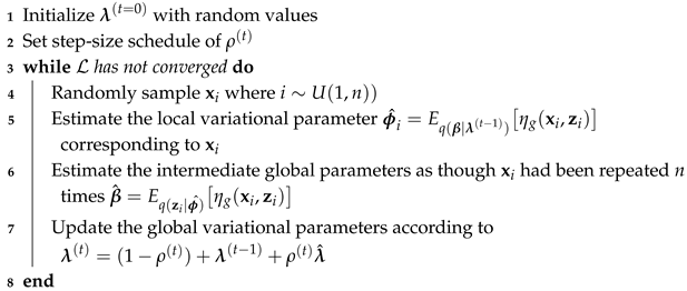 |
Appendix B.3. Black Box Variational Inference
One of the most challenging aspects of using variational inference methods is the tedious derivation of algorithms for each specific class of models. Compounding this challenge is the fact that an analytical solution for the ELBO is typically not even possible for models outside of the conditionally conjugate exponential family. Fortunately, a technique known as black box variational inference (BBVI), first introduced by [45], alleviates both of these issues by using Monte Carlo samples from the variational distribution to attain “noisy” (stochastic) estimates of the ELBO gradient, even in cases where the ELBO has no analytical solution. When coupled with techniques such as automatic differentiation, we can entirely side step the process of tedious gradient derivations for most models, regardless of whether or not their ELBO functions are analytically tractable.
Suppose that we have our set of observations as and as our latent variables with joint density . Furthermore, suppose that we have variational density , where denotes our set of variational parameters. From (A22), it follows that the generic form of the ELBO is as follows:
whose gradient with respect to the variational parameter is given as follows:
Note that this interchange of the expectation and gradient is valid, provided that the score function exists and the score and likelihood are bounded [45]. By interchanging the expectation and gradient in (A30), we obtain the following:
we can attain an unbiased estimator of the ELBO by computing the following:
where is a Monte Carlo sample from variational density . The results of (A32) can be leveraged to develop the stochastic optimization algorithm shown in Algorithm 2. In cases where the Monte Carlo gradient in (A32) exhibits high variance, Rao–Blackwellization can be employed to make the gradient estimates less noisy.
| Algorithm 2: Generic BBVI Algorithm [45] |
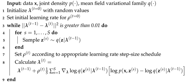 |
References
- Malki, A.; Atlam, E.S.; Gad, I. Machine learning approach of detecting anomalies and forecasting time-series of IoT devices. Alex. Eng. J. 2022, 61, 8973–8986. [Google Scholar] [CrossRef]
- Zhang, D.; Lindholm, G.; Ratnaweera, H. Use long short-term memory to enhance Internet of Things for combined sewer overflow monitoring. J. Hydrol. 2018, 556, 409–418. [Google Scholar] [CrossRef]
- Toman, P.; Soliman, A.; Ravishanker, N.; Rajasekaran, S.; Lally, N.; D’Addeo, H. Understanding insured behavior through causal analysis of IoT streams. In Proceedings of the 2023 6th International Conference on Data Mining and Knowledge Discovery (DMKD 2023), Seoul, Republic of Korea, 17–19 March 2023. [Google Scholar]
- Soliman, A.; Rajasekaran, S.; Toman, P.; Ravishanker, N.; Lally, N.G.; D’Addeo, H. A custom unsupervised approach for pipe-freeze online anomaly detection. In Proceedings of the 2021 IEEE 7th World Forum on Internet of Things (WF-IoT), New Orleans, LA, USA, 14 June– 31 July 2021; pp. 663–668. [Google Scholar]
- Box, G.E.; Tiao, G.C. Intervention analysis with applications to economic and environmental problems. J. Am. Stat. Assoc. 1975, 70, 70–79. [Google Scholar] [CrossRef]
- Abraham, B. Intervention analysis and multiple time series. Biometrika 1980, 67, 73–78. [Google Scholar] [CrossRef]
- Aminikhanghahi, S.; Cook, D.J. A survey of methods for time series change point detection. Knowl. Inf. Syst. 2017, 51, 339–367. [Google Scholar] [CrossRef]
- Brodersen, K.H.; Gallusser, F.; Koehler, J.; Remy, N.; Scott, S.L. Inferring causal impact using Bayesian structural time-series models. Ann. Appl. Stat. 2015, 9, 247–274. [Google Scholar] [CrossRef]
- Scott, S.L.; Varian, H.R. Predicting the present with Bayesian structural time series. Int. J. Math. Model. Numer. Optim. 2014, 5, 4–23. [Google Scholar] [CrossRef]
- Williams, C.K.; Rasmussen, C.E. Gaussian Processes for Machine Learning; MIT Press: Cambridge, MA, USA, 2006; Volume 2. [Google Scholar]
- Corani, G.; Benavoli, A.; Zaffalon, M. Time series forecasting with Gaussian processes needs priors. In Joint European Conference on Machine Learning and Knowledge Discovery in Databases; Springer: Cham, Switzerland, 2021; pp. 103–117. [Google Scholar]
- Roberts, S.; Osborne, M.; Ebden, M.; Reece, S.; Gibson, N.; Aigrain, S. Gaussian processes for time-series modelling. Philos. Trans. R. Soc. A Math. Phys. Eng. Sci. 2013, 371, 20110550. [Google Scholar] [CrossRef] [PubMed]
- Duvenaud, D.; Lloyd, J.; Grosse, R.; Tenenbaum, J.; Zoubin, G. Structure discovery in nonparametric regression through compositional kernel search. In Proceedings of the International Conference on Machine Learning, PMLR, Atlanta, GA, USA, 17–19 June 2013; pp. 1166–1174. [Google Scholar]
- Wilson, A.; Adams, R. Gaussian process kernels for pattern discovery and extrapolation. In Proceedings of the International Conference on Machine Learning, PMLR, Atlanta, GA, USA, 17–19 June 2013; pp. 1067–1075. [Google Scholar]
- Brahim-Belhouari, S.; Bermak, A. Gaussian process for nonstationary time series prediction. Comput. Stat. Data Anal. 2004, 47, 705–712. [Google Scholar] [CrossRef]
- Durbin, J.; Koopman, S.J. Time Series Analysis by State Space Methods; OUP Oxford: Oxford, UK, 2012; Volume 38. [Google Scholar]
- Shumway, R.H.; Stoffer, D.S.; Stoffer, D.S. Time Series Analysis and its Applications, 3rd ed.; Springer: Berlin/Heidelberg, Germany, 2011. [Google Scholar]
- West, M.; Harrison, J. Bayesian Forecasting and Dynamic Models; Springer Science & Business Media: Berlin/Heidelberg, Germany, 2006. [Google Scholar]
- Frigola, R.; Lindsten, F.; Schön, T.B.; Rasmussen, C.E. Bayesian inference and learning in Gaussian process state-space models with particle MCMC. Adv. Neural Inf. Process. Syst. 2013, 26. Available online: https://arxiv.org/abs/1306.2861 (accessed on 23 May 2025).
- Doerr, A.; Daniel, C.; Schiegg, M.; Duy, N.T.; Schaal, S.; Toussaint, M.; Sebastian, T. Probabilistic recurrent state-space models. In Proceedings of the International Conference on Machine Learning, PMLR, Stockholm, Sweden, 10–15 July 2018; pp. 1280–1289. [Google Scholar]
- Deisenroth, M.P.; Huber, M.F.; Hanebeck, U.D. Analytic moment-based Gaussian process filtering. In Proceedings of the 26th Annual International Conference on Machine Learning, Montreal, QC, Canada, 14–18 June 2009; pp. 225–232. [Google Scholar]
- Turner, R.; Deisenroth, M.; Rasmussen, C. State-space inference and learning with Gaussian processes. In Proceedings of the Thirteenth International Conference on Artificial Intelligence and Statistics, JMLR Workshop and Conference Proceedings, Sardinia, Italy, 13–15 May 2010; pp. 868–875. [Google Scholar]
- Frigola, R.; Chen, Y.; Rasmussen, C.E. Variational Gaussian process state-space models. Adv. Neural Inf. Process. Syst. 2014, 27. Available online: https://arxiv.org/abs/1406.4905 (accessed on 23 May 2025).
- Blei, D.M.; Kucukelbir, A.; McAuliffe, J.D. Variational inference: A review for statisticians. J. Am. Stat. Assoc. 2017, 112, 859–877. [Google Scholar] [CrossRef]
- Eleftheriadis, S.; Nicholson, T.; Deisenroth, M.; Hensman, J. Identification of Gaussian process state space models. Adv. Neural Inf. Process. Syst. 2017, 30. Available online: https://arxiv.org/abs/1705.10888 (accessed on 23 May 2025).
- Ialongo, A.D.; Van Der Wilk, M.; Hensman, J.; Rasmussen, C.E. Overcoming mean-field approximations in recurrent Gaussian process models. In Proceedings of the International Conference on Machine Learning, PMLR, Long Beach, CA, USA, 9–15 June 2019; pp. 2931–2940. [Google Scholar]
- Toman, P.; Ravishanker, N.; Lally, N.; Rajasekaran, S. Latent autoregressive Student-t prior process models to assess impact of interventions in time series. Future Internet 2023, 16, 8. [Google Scholar] [CrossRef]
- West, M. On scale mixtures of normal distributions. Biometrika 1987, 74, 646–648. [Google Scholar] [CrossRef]
- Ravishanker, N.; Chi, Z.; Dey, D.K. A First Course in Linear Model Theory; Chapman and Hall/CRC: Boca Raton, FL, USA, 2021. [Google Scholar]
- Schuster, M.; Paliwal, K.K. Bidirectional recurrent neural networks. IEEE Trans. Signal Process. 1997, 45, 2673–2681. [Google Scholar] [CrossRef]
- Paszke, A.; Gross, S.; Massa, F.; Lerer, A.; Bradbury, J.; Chanan, G.; Killeen, T.; Lin, Z.; Gimelshein, N.; Antiga, L.; et al. Pytorch: An imperative style, high-performance deep learning library. Adv. Neural Inf. Process. Syst. 2019, 32. Available online: https://arxiv.org/abs/1912.01703 (accessed on 23 May 2025).
- Gardner, J.; Pleiss, G.; Weinberger, K.Q.; Bindel, D.; Wilson, A.G. Gpytorch: Blackbox matrix-matrix Gaussian process inference with gpu acceleration. Adv. Neural Inf. Process. Syst. 2018, arXiv:1809.11165. [Google Scholar] [CrossRef]
- Lin, Z.; Cheng, L.; Yin, F.; Xu, L.; Cui, S. Output-Dependent Gaussian Process State-Space Model. In Proceedings of the ICASSP 2023—2023 IEEE International Conference on Acoustics, Speech and Signal Processing (ICASSP), Rhodos, Greece, 4–10 June 2023; pp. 1–5. [Google Scholar]
- Gneiting, T.; Raftery, A.E. Strictly proper scoring rules, prediction, and estimation. J. Am. Stat. Assoc. 2007, 102, 359–378. [Google Scholar] [CrossRef]
- Lloyd, J.; Duvenaud, D.; Grosse, R.; Tenenbaum, J.; Ghahramani, Z. Automatic construction and natural-language description of nonparametric regression models. In Proceedings of the AAAI Conference on Artificial Intelligence, Québec City, QC, Canada, 27–31 July 2014; Volume 28. [Google Scholar]
- Snelson, E.; Ghahramani, Z. Sparse Gaussian processes using pseudo-inputs. Adv. Neural Inf. Process. Syst. 2005, 18. Available online: https://papers.nips.cc/paper_files/paper/2005/hash/4491777b1aa8b5b32c2e8666dbe1a495-Abstract.html (accessed on 23 May 2025).
- Titsias, M. Variational learning of inducing variables in sparse Gaussian processes. In Proceedings of the Artificial Intelligence and Statistics, PMLR, Clearwater Beach, FL, USA, 16–18 April 2009; pp. 567–574. [Google Scholar]
- Hensman, J.; Fusi, N.; Lawrence, N.D. Gaussian processes for big data. arXiv 2013, arXiv:1309.6835. [Google Scholar]
- Hensman, J.; Matthews, A.; Ghahramani, Z. Scalable variational Gaussian process classification. In Proceedings of the Artificial Intelligence and Statistics, PMLR, San Diego, CA, USA, 9–12 May 2015; pp. 351–360. [Google Scholar]
- Girard, A.; Rasmussen, C.E.; Quinonero-Candela, J.; Murray-Smith, R.; Winther, O.; Larsen, J. Multiple-step ahead prediction for non-linear dynamic systems—A Gaussian process treatment with propagation of the uncertainty. Adv. Neural Inf. Process. Syst. 2002, 15, 529–536. [Google Scholar]
- Mattos, C.L.C.; Damianou, A.; Barreto, G.A.; Lawrence, N.D. Latent autoregressive Gaussian processes models for robust system identification. IFAC-PapersOnLine 2016, 49, 1121–1126. [Google Scholar] [CrossRef]
- Lee, H.; Yun, E.; Yang, H.; Lee, J. Scale mixtures of neural network Gaussian processes. arXiv 2021, arXiv:2107.01408. [Google Scholar]
- Hoffman, M.D.; Blei, D.M.; Wang, C.; Paisley, J. Stochastic variational inference. J. Mach. Learn. Res. 2013, 14, 1303–1347. [Google Scholar]
- Bishop, C.M.; Nasrabadi, N.M. Pattern Recognition and Machine Learning; Springer: Berlin/Heidelberg, Germany, 2006; Volume 4. [Google Scholar]
- Ranganath, R.; Gerrish, S.; Blei, D. Black box variational inference. In Proceedings of the Artificial Intelligence and Statistics, PMLR, Valencia, Spain, 22–25 April 2014; pp. 814–822. [Google Scholar]


Disclaimer/Publisher’s Note: The statements, opinions and data contained in all publications are solely those of the individual author(s) and contributor(s) and not of MDPI and/or the editor(s). MDPI and/or the editor(s) disclaim responsibility for any injury to people or property resulting from any ideas, methods, instructions or products referred to in the content. |
© 2025 by the authors. Licensee MDPI, Basel, Switzerland. This article is an open access article distributed under the terms and conditions of the Creative Commons Attribution (CC BY) license (https://creativecommons.org/licenses/by/4.0/).