Stochastic Model and Rhythm-Adaptive Technologies of Statistical Analysis and Forecasting of Economic Processes with Cyclic Components

Abstract

This article presents a mathematical model of cyclical economic processes, formulated as the sum of a deterministic polynomial function and a cyclic random process that simultaneously captures trend, stochasticity, cyclicity, and rhythm variability. Building on this stochastic framework, we propose rhythm-adaptive statistical techniques for estimating the probabilistic characteristics of the cyclic component; by adjusting to rhythm changes, these techniques improve estimation accuracy. We also introduce a forecasting procedure that constructs a system of rhythm-adaptive confidence intervals for future cycles. The effectiveness of the model and associated methods is demonstrated through a series of computational experiments using Federal Reserve Economic Data. Results show that the rhythm-adaptive forecasting approach achieves mean absolute errors less than half of those produced by a comparable non-adaptive method, underscoring its practical advantage for the analysis and prediction of cyclic economic phenomena.

1. Introduction

The accelerating progress of information technologies—especially in data science, signal processing, and machine-learning—has spurred the development of increasingly effective tools for modeling, analyzing, and forecasting economic time series. Among these series, cyclical economic processes, whose trajectories exhibit recurrent patterns of expansion and contraction, are of particular interest for policy and business decision-making.

Theoretical insight into economic cycles has evolved from the seminal ideas of Karl Marx, Clementon Joulliar, Tugan-Baranovsky, Joseph Kitchin, N. D. Kondratiev, Van Gelderen, Pitirim Sorokin, Joseph Schumpeter, Michal Kalecki, Nicholas Kaldor, J. R. Hicks, Simon Kuznets, Paul Samuelson, W. W. Rostow, Jay Forrester, Christopher Freeman, Gerhard Mensch, Alfred Klinknecht, A. L. Gelfand, V. G. Klinov, Yu. V. Yakovets, Bruce E. Hansen, Jacob van Dijn, Gary van Vuuren, Robert J. Hodrick [1], Neil Kang, Victor Marmer [2], Łukasz Lenart, Łukasz Kwiatkowski, Justyna Wróblewska [3], Jens J. Krüger [4], Fatih Guvenen, Alisdair McKay, Carter Ryan [5], Marius Wildi [6], Willi Semmler, Thomas Palley [7], Eder Luiz Pontes, Mohamed Benjannet, Richard Yung [8], Antonio Azqueta-Gavaldon, Daniel Hirschbühl, Luca Onorante, Laura Saiz [9], and Volker Kuntze [10].

The use of modern software tools for modeling, analysis and forecasting of cyclic economic processes significantly complements, strengthens and intensifies the decision-making process of economist specialists. Among the large collection of software systems for the analysis and forecasting of economic cyclical phenomena, the following can be named:

• Software specializing in econometrics, regression analysis, and time series analysis: EViews (Quantitative Micro Software), Stata (StataCorp LLC), Rats (Thomas Doan and Robert Littermn), Micro TSP (David M. Lilien), Gretl (Riccardo “Jack” Lucchetti, Allin Cottrell).
• Software for statistical analysis, descriptive statistics, regression, and factor analysis: IBM SPSS (Normn H.Nie), SAS (James Goodnight), BMDP Statistical Soft¬ware (W.J.Dixon), Minitab (Minitab Inc.).
• Programming languages and libraries for statistics, machine learning, and econometric modeling: Python (Libraries: statsmodels, scikit-learn, pmdarima, PyWavelets), R (packages: forecast, tseries, vars, wavelets).
• Tools for business analytics, financial forecasting, and simulation modeling: Oracle Crystal Ball (Oracle Corporation), Tableau (Tableau Software).

Conventionally, three main paradigms for the modeling, analysis and forecasting of cyclic economic processes can be distinguished, namely: the model-based paradigm, data-based paradigm (data-driving or data-oriented paradigm), and a hybrid paradigm that integrates the first two paradigms. The model-based paradigm is historically the first and is based on the development and justification of mathematical models of cyclic economic phenomena that reflect the essential properties of their structure. Based on pre-developed mathematical models of cyclic economic processes, methods and algorithms for their analysis and forecasting are created deductively. The data-driving paradigm does not require the construction of a mathematical model of cyclic economic processes, but focuses directly on the structural-parametric identification of algorithms for their analysis and forecasting using machine learning methods, in particular deep machine learning methods, based on real economic data. The hybrid paradigm in a certain way combines model-based and data-based paradigms, trying to increase the accuracy, reliability, speed and level of interpretability of algorithms for the analysis and forecasting of cyclic economic processes. We will briefly consider the state of affairs in this area from the standpoint of these three paradigms.

2. Related Work

Since the conceptual cores that determines the accuracy, reliability and computational complexity of model-based technologies for the analysis and forecasting of cyclical economic processes are their corresponding mathematical models, we will briefly consider their main classes.

Within the framework of model-based technologies, various classes of mathematical models are distinguished: deterministic and stochastic, crisp and fuzzy models, interval models, GMDH (Group Method of Data Handling) models, “Caterpillar method” models, fractal models. Within the deterministic approach, in article [11], financial market time series were analyzed using dynamic Fourier transformation and wavelet analysis to identify cyclicality, volatility, and structural changes in the data. In paper [4], wavelet analysis was applied to assess key business cycle indicators of the German economy, focusing on their frequency components and time-varying characteristics to improve economic cycle forecasting. In article [12], the forecasting of the zakat collection in Lembaga Zakat Negeri Kedah for 2023 was examined using the Holt-Winters exponential smoothing method. Seasonal trends in data from 2016 to 2022 were analyzed, additive and multiplicative models were compared, and it was concluded that the additive model provides higher accuracy for financial planning. In the article [6], the Simple Sign Accuracy (SSA) model was presented as a deterministic framework for optimizing predictions of zero-crossings in stationary time series by balancing accuracy, timeliness, and smoothness through mathematically defined holding time constraints. It is worth noting that within the framework of the deterministic approach, deterministic functions are used as mathematical models of cyclic economic processes and are, in particular, used with harmonic functions, polyharmonic periodic functions, and almost periodic deterministic functions. These deterministic models are relatively simplified and idealized representations of real economic phenomena.

Stochastic mathematical models of cyclic economic processes include stochastic periodic autoregressive and moving average models, which have been studied by Tiao and Grupe (1980) [13], Todd (1983, 1990) [14,15], Osborn (1988) [16], Osborn and Smith (1989) [17], Hansen and Sargent (1990) [18], and Dolado et al. (2022) [19]. A family of ARIMA [20], SARIMA, and ARIMAX models was utilized by Hyndman (2021) [21] and Choi (2018) [22]. Regarding VAR and VECM models, noteworthy contributions include Krolzig (1998) [23], Cogley, Amisano (2013) [24], and Choi, Kim (2023) [25]. Additionally, periodic random Markov processes and chains were investigated by Ghysels (1991b, 1992) [26,27], Hamilton (1988, 1989, 1990) [28,29,30], Garcia and Perron (1989) [31], Phillips (1991) [32], McCulloch and Tsay (1992) [33], Albert and Chib (1993) [34], Robert J. Hodrick (2020) [1], McCracken M. W., Owyang M. T., Sekhposyan T. (2021) [35], Fatih Guvenen, Alisdair McKay, Carter Ryan (2023) [5], Marius Wildi (2024) [6], Bernard L., Gevorkyan A., Palley T., Semmler W. (2024) [7], Lenart Ł., Kwiatkowski Ł., Wróblewska J. (2024) [3]. In article [36], a forecast of Jordan’s GDP for 2022–2031 is analyzed using a combination of Wavelet Transform and ARIMA models to support economic planning. The dynamics of the Gross Domestic Product (GDP) of Dongying City (China) from 1978 to 2016 and its forecast for 2017–2020, performed using the ARIMA model, are discussed in article [20]. The article also addresses the specific features of resource-dependent cities’ economies and the strategic challenges arising from reliance on natural resources.

In article [37], the economic growth of the Republic of Moldova over the period of 1967–2019 is analyzed using the ARIMA model. The study explores the relationship between innovation, technological development, and macroeconomic stability to foster the development of an innovative economy. In article [38], the modeling and forecasting of PepsiCo’s stock prices using ARIMA models are explored. The study demonstrates the use of the R programming language for time series analysis, graph construction, optimal model parameter selection, and accurate forecasting, enabling effective decision-making in the financial market.

In article [39], the dynamics and forecasting of China’s Gross Domestic Product (GDP) are studied using the ARIMA model, analyzing data from 1978 to 2022 and forecasting economic development for 2023–2027. The study concludes that the selected ARIMA (0, 2, 0) model provides high forecasting accuracy. Recommendations for stimulating economic growth are proposed, including fostering innovation, attracting highly skilled professionals, optimizing the industrial structure, and deepening international cooperation. In article [40], a combined model is utilized, integrating autocorrelated Logit models, dynamic factor models, and MIDAS (Mixed-Data Sampling) regression. This model aims to forecast recessions in business cycles using less restrictive target variables to determine the probability of a recession occurring within a specific time interval. Such an approach enhances prediction accuracy and enables the timely identification of turning points in the economic cycle. The relationship between stock market volatility and the financial cycle in Vietnam was analyzed in article [41] using GARCH family models, including EGARCH, TGARCH, and GJR-GARCH. Utilizing VNIndex data from 2000 to 2020, the authors identify key patterns of market volatility, explore the mechanisms of financial cycles, and assess the potential for forecasting significant economic events. In the article [42], the development and application of a Composite Leading Indicator (CLI) for forecasting economic growth in Hong Kong using a Vector Autoregression (VAR) model were highlighted. Special attention was given to adapting the indicators to changes caused by the COVID-19 pandemic and improving forecast accuracy by accounting for the new economic conditions. In article [35], the use of the Mixed-Frequency Bayesian VAR (MF-BVAR) model for real-time economic forecasting and scenario analysis is analyzed. The primary focus is on integrating data from different frequencies (monthly and quarterly indicators) to forecast real GDP growth and assess the impact of hypothetical changes in political or economic conditions. Forecasting cyclic economic processes is performed using Markov Chains in paper [43]. The method is applied to analyze and assess the financial stability of enterprises, particularly for modeling potential changes in a company’s financial condition depending on economic conditions.

In the last decade, the expansion of data-based approaches in the analysis and forecasting of cyclical economic processes has been particularly active. For example, machine learning is used to forecast consumer confidence in China and analyze business cycles [44,45]. In the study of time series, such approaches allow for the modeling complex of nonlinear dependencies, providing more accurate forecasts compared to traditional methods [46,47]. The use of deep learning and optimization has shown high efficiency in forecasting gold prices and exchange rates [48,49]. In addition, innovative approaches to the analysis of probability distributions and forecasting recessions in macroeconomics demonstrate the potential of using big data for a deeper understanding of economic cycles [50,51,52]. Forecasting the phases of business cycles using machine learning methods, which include the analysis of stock indicators and the construction of network structures, is an effective real-time tool for identifying turning points in economic activity [8,9]. In addition, the use of models that take into account the relationship between business cycles, credit cycles and investments allow for more stable forecasts, in particular for economies such as India [53]. Thus, modern information technologies based on machine learning algorithms provide multidimensional analysis and create new opportunities for decision-making in the economy.

Within the framework of the hybrid paradigm, the integration of ARIMA models with neural networks and weighted fuzzy membership functions was carried out, which made it possible to effectively forecast business cycles taking into account nonlinear effects on the economic system [54]. The use of wavelet transformation and artificial neural networks makes it possible to take into account the multi-level structure of financial time series [55]. Other approaches, such as advanced dynamic modal decomposition, provide a deeper analysis of macroeconomic cycles by merging traditional mathematical models with machine learning algorithms [56]. Thus, the hybrid approach combines the advantages of traditional models and modern data-driving technologies, providing tools for more accurate assessment and forecasting of economic processes.

Model-based and hybrid paradigms require the preliminary development of a mathematical model of cyclical economic processes, the quality (adequacy, informativeness) of which will significantly affect the characteristics of accuracy, reliability, computational complexity and interpretability of algorithms and software systems for analysis, forecasting and support of economic decision-making according to cyclical economic processes.

Table 1. Comparative table of mathematical models for cyclic economic processes as formalized tools of information systems for their analysis, forecasting, and simulation.

			Properties of cyclic economic processes accounted for by the mathematical model
			Cyclic structure of cyclic economic processes	Randomness of the structure of cyclic economic processes	Variability of rhythm	Commonality of rhythm	Trend components
Known mathematical models	Deterministic	FOURIER SERIES AND FOURIER TRANSFORM	+	−	−	−	−
		WAVELET SERIES AND WAVELET TRANSFORM	+	−	+	−	−
		SIMPLE SIGN ACCURACY (SSA)	−	−	−	−	+
		WINTERS’ EQUATIONS	+	−	−	−	+
	Stochastic	REGRESSION MODELS	−	+	−	−	+
		STATIONARY RANDOM PROCESS	−	+	−	−	−
		PERIODIC ARMA MODELS	+	+	−	−	−
		ARIMA, SARIMA, ARIMAX	+	+	−	−	+
		GARCH, ARCH, EGARCH	−	+	−	−	−
		VAR, VECM	−	+	−	+	−
		AR-LOGIT-FACTOR-MIDAS	+	+	−	+	+
		PERIODIC MARKOV CHAINS	+	+	−	−	−
	Other models	NEURAL NETWORK MODELS	+	−	−	−	+
		MODELS IN THE “CATERPILLAR” METHOD	+	+	−	−	+
		FUZZY MODELS	+	−	−	−	+
		MODELS IN GMDH (GROUP METHOD OF DATA HANDLING)	−	+	−	−	+
		INTERVAL MODELS	−	−	−	−	+
New models		SUM OF A POLYNOMIAL FUNCTION AND A CYCLIC RANDOM PROCESS	+	+	+	−	+
		SUM OF VECTORS OF POLYNOMIAL FUNCTIONS AND A VECTOR OF CYCLICALLY RHYTHMICALLY CONNECTED RANDOM PROCESSES	+	+	+	+	+

shows the comparative characteristics of known and new mathematical models of cyclical economic processes.

In summary, quantitative modeling in economic-cycle theory has advanced from deterministic formulations to increasingly complex stochastic and machine learning approaches. Deterministic models offer high interpretability but limited flexibility, whereas stochastic models such as ARIMA and GARCH capture randomness yet still assume fixed periodicity. Machine learning methods improve predictive accuracy but often at the cost of transparency and explainability. A detailed side-by-side comparison of these approaches with the proposed model is provided in Table 1. Building on this evolutionary path, our method introduces a rhythm-adaptive stochastic framework that balances accuracy, computational efficiency, and interpretability. By explicitly modeling rhythm variability—a feature overlooked in most existing approaches—our model offers a versatile new tool for the statistical analysis and forecasting of economic cycles.

As can be seen in Table 1, the model of cyclic economic processes developed and studied in the article in the form of a sum of polynomial function and a cyclic random process has significant advantages over known models, in particular, in comparison with stochastic periodic models, which include periodic autoregressive models and periodic Markov chains, which is justified by taking into account in the new model, in addition to the stochastic nature of economic processes and their cyclical structure, as well as the variability of the rhythm of cyclical components of economic processes, which reflects the specificity of the “own time of the economic system”. Also, this mathematical model of the economic process can be generalized to several interconnected cyclical economic processes, where the sum of the vector of polynomial functions and the vector of cyclically rhythmically connected random processes will be an adequate model.

The work is devoted to mathematical modeling and rhythm-adaptive methods of statistical analysis and the forecasting of cyclical economic processes within the framework of the theory of cyclic random processes. The creation of such a model and methods of processing economic processes will make it possible to increase the accuracy, reliability, speed and level of interpretability of the economic decision-making support technology.

3. Methodology

3.1. Mathematical Models of a Cyclical Economic Process

Typical examples of cyclical economic processes include unemployment rates, imports of high-technology goods, and seasonal income indices (Figure 1). Graphs B and D illustrate the downturn that followed the COVID-19 recession, whereas Graph C highlights contractions driven by the 1990s recession, the dot-com crash, and the 2008 financial crisis.

Taking into account the peculiarities of the structure of cyclical economic processes, we demand that the model take into account their stochastic nature, trend character, the presence of a cyclical component and the variability of the oscillation rhythm associated with the variability of the economic system’s own time, where the studied processes take place. In addition, the model should have formal means of displaying the detailed phase structure of economic cycles. Also, the mathematical model should make it possible to describe, analyze and forecast cyclical economic processes in both the continuous and discrete time domains. The model should be suitable for the analysis of cyclical economic processes both within the framework of the spectral-correlation theory of random processes and within the framework of higher-order moment functions and distribution functions.

Taking into account the above requirements, we will use the additive model

$$y\left(\omega ,t\right)=\sum _{j=0}^J{c}_j·t^j+\xi \left(\omega ,t\right),\omega \in \mathsf{\Omega },t\in \mathit{R},$$

(1)

as a mathematical model of cyclic economic processes of a continuous parameter;

and we will use the additive model

$$y\left(\omega ,t_{m,l}\right)=\sum _{j=0}^J{c}_j·t_{m,l}^j+\xi \left(\omega ,t_{m,l}\right),\omega \in \mathit{\Omega },t_{m,l}\in \mathit{D}.$$

(2)

as a mathematical model of cyclical economic processes of a discrete parameter.

In models (1) and (2), polynomials of the $N$-th order $\sum _{j=0}^J{c}_j·t^j$ and $\sum _{j=0}^J{c}_j·t_{m,l}^j$ reflect trend deterministic components of the economic process, and components $\xi \left(\omega ,t\right)$ and $\xi \left(\omega ,t_{m,l}\right)$ are cyclic random processes (or cyclically correlated random processes) [57,58] that reflect cyclic stochastic components of the studied economic processes. The discrete domain definition, $\mathit{D}\subset \mathit{R}$, of cyclic (cyclically correlated) random process $\xi \left(\omega ,t_{ml}\right)$ is the set of isolated real numbers, namely, a set $\mathit{D}=\left\{t_{m,l}:t_{m,l}\in \mathit{R},m\in \mathit{Z},l=\overline{1,L},L\ge 2\right\}$, for the elements for which the following type of linear ordering exits: if $m_2>m_1$ or if $m_2=m_1$ and $l_2>l_1$, then $t_{m_1,l_1}<t_{m_2{,l}_2}$; in other cases: $t_{m_1{,l}_1}>t_{m_2{,l}_2}$ ($m_2,m_1\in \mathit{Z},l_1,l_2=\overline{1,L}, 0<t_{m+1,l}-t_{m,l}<\infty$). Set $\mathit{\Omega }$ is a set of elementary events.

According to works [57,58,59] we briefly define and state the fundamental properties of a cyclically correlated random process and a cyclic random process of both continuous and discrete parameters.

Definition 1.

The random process$\xi \left(\omega ,t\right),\omega \in \mathit{\Omega },t\in \mathit{R}$ is called the cyclically correlated random process of a continuous parameter, if for its mathematical expectation$m_{\xi }\left(t\right)$ and autocovariance function$R_{\xi }^2\left(t_1,t_2\right)$, there exists a such function$T\left(t,n\right), t\in \mathit{R}, n\in \mathit{Z}$, which satisfies the conditions (5)–(7) of the rhythm function, and there are following equalities:

$$m_{\xi }\left(t\right)=m_{\xi }\left(t+T\left(t,n\right)\right),t\in \mathit{R},n\in \mathit{Z},$$

(3)

$$R_{\xi }^2\left(t_1,t_2\right)=R_{\xi }^2\left(t_1+T\left(t_1,n\right),t_2+T\left(t_2,n\right)\right),t_1,t_2\in \mathit{R},n\in \mathit{Z}.$$

(4)

The rhythm function $T\left(t,n\right), t\in \mathit{R}, n\in \mathit{Z}$ has the following properties [35,36,37]:

(1):

$$\left\{\begin{array}{c}T\left(t,n\right)>0 \left(T\left(t,1\right)<\infty \right),t\in \mathit{R},if n>0, \\ T\left(t,n\right)=0,t\in \mathit{R},if n=0, \\ T\left(t,n\right)<0,t\in \mathit{R},if n<0; \end{array}\right.$$

(5)

(2) for any $t_1\in \mathit{R}$ and $t_2\in \mathit{R}$, for which $t_1<t_2$, for function $T\left(t,n\right)$ a strict inequality holds:

$$T\left(t_1,n\right)+t_1<T\left(t_2,n\right)+t_2,\forall n\in \mathit{Z};$$

(6)

(3) function $T\left(t,n\right)$ is the smallest in modulus $\left( \left|T\left(t,n\right)\right|\le \left|T_{\gamma }\left(t,n\right)\right|\right)$ among all such functions $\left\{T_{\gamma }\left(t,n\right),\gamma \in \mathit{N}\right\}$ which satisfy (5) and (6), namely:

$$\left|T\left(t,n\right)\right|={min}_{\gamma \in \mathit{N}}\left\{\left|T_{\gamma }\left(t,n\right)\right|,\gamma \in \mathit{N}\right\},t\in \mathit{R}, n\in \mathit{Z}.$$

(7)

The rhythm function $T\left(t,n\right)$ determines the law of changing the time intervals between the single-phase values of the cyclically correlated random process.

A cyclically correlated random process of a continuous parameter has the ability to explore only the mathematical expectation and the autocovariance function of cyclic economic processes. However, in many applied situations, it is necessary to have information about other probabilistic characteristics and, in particular, about moment functions of a higher order and about distribution functions of the studied economic processes. In this case, an adequate mathematical model of these cyclic economic processes is a cyclic random process (cyclically distributed random process) of a continuous parameter.

Definition 2.

The separable random process$\xi \left(\omega ,t\right),\omega \in \mathit{\Omega },t\in \mathit{R}$ is called the cyclic random process (cyclically distributed random process) of a continuous parameter, if for it there exists such a function$T\left(t,n\right), t\in \mathit{R}, n\in \mathit{Z}$ which satisfies conditions (5)–(7) of the rhythm function, and for any$t_1,\dots ,t_k$ from the set of separability of the process$\xi \left(\omega ,t\right),\omega \in \mathit{\Omega },t\in \mathit{R}$,$k$-dimensional random vectors$\left(\xi \left(\omega ,t_1\right),\dots ,\xi \left(\omega ,t_k\right)\right)$ and$\left(\xi \left(\omega ,t_1+T\left(t_1,n\right)\right),\dots ,\xi \left(\omega ,t_k+T\left(t_k,n\right)\right)\right)$ are stochastically equivalent in the wide sense for all$n\in \mathit{Z}$ and for all$k\in \mathit{N}$.

Note that $k$-dimensional random vectors will be stochastically equivalent in the wide sense, if they are the same $k$-dimensional distribution functions. For $k$-dimensional distribution function $F_{\xi }^k\left(x_1,\dots ,x_k,t_1,\dots ,t_k\right)$ from the family of consistent distribution functions of a cyclic random process $\xi \left(\omega ,t\right),\omega \in \mathit{\Omega },t\in \mathit{R}$ there are following equalities:

$$\begin{gathered} F_{\xi }^k\left(x_1,\dots ,x_k,t_1,\dots ,t_k\right)=F_{\xi }^k\left(x_1,\dots ,x_k,t_1+T\left(t_1,n\right),\dots ,t_k+T\left(t_k,n\right)\right), \\ {x}_1,\dots ,x_k,t_1,\dots ,t_k\in \mathit{R},n\in \mathit{Z},k\in \mathit{N}. \end{gathered}$$

(8)

Given the existence of corresponding moment functions of a cyclic random process of continuous parameters, these moment functions have the following dependencies. The mixed initial moment function $C_{\xi }^p\left(t_1,\dots ,t_k\right)$ of order $p={\sum }_{j=1}^k{r}_j$ of cyclic random process $\xi \left(\omega ,t\right)$ satisfies the following equality:

$$\begin{gathered} C_{\xi }^p\left(t_1,\dots ,t_k\right)=\mathit{E}\left\{\prod _{j=1}^k{\left(\xi \left(\omega ,t_j\right)\right)}^{r_j}\right\}= \\ =C_{\xi }^p\left(t_1+T\left(t_1,n\right),\dots ,t_k+T\left(t_k,n\right)\right),\hspace{0.33em}{t}_1,\dots ,t_k\in \mathit{R},\hspace{0.33em}n\in \mathit{Z},k\in \mathit{N}. \end{gathered}$$

(9)

The mixed central moment function $R_{\xi }^p\left(t_1,\dots ,t_k\right)$ of order $p={\sum }_{j=1}^k{r}_j$ of cyclic random process $\xi \left(\omega ,t\right)$ satisfies the following equality:

$$\begin{gathered} R_{\xi }^p\left(t_1,\dots ,t_k\right)=\mathit{E}\left\{\prod _{j=1}^k{\left(\xi \left(\omega ,t_j\right)-m_{\xi }\left(t_j\right)\right)}^{r_j}\right\}= \\ =R_{\xi }^p\left(t_1+T\left(t_1,n\right),\dots ,t_k+T\left(t_k,n\right)\right),t_1,\dots ,t_k\in \mathit{R},\hspace{0.33em}n\in \mathit{Z},k\in \mathit{N}. \end{gathered}$$

(10)

If in (9) $k=1$ and $r_1=1$($p=1$) we will have the initial moment function of the first order (mathematical expectation) $C_{\xi }^1\left(t\right)=m_{\xi }\left(t\right)$ of the cyclic random process $\xi \left(\omega ,t\right)$. If in (9) $k=2$ and $r_1=r_2=1$($p=2$) we will have a mixed initial moment function of the second order (autocorrelation function) $C_{\xi }^2\left(t_1,t_2\right)$ of the cyclic random process $\xi \left(\omega ,t\right)$. If in (10) $k=1$ and $r_1=2$($p=2$) we will have a central moment function of the second order (variance) $R_{\xi }^2\left(t,t\right)=d_{\xi }^2\left(t\right)$ of the cyclic random process $\xi \left(\omega ,t\right)$. If, in (10), $k=2$ and $r_1=r_2=1$($p=2$) we will have a mixed central moment function of the second order (autocovariance function) $R_{\xi }^2\left(t_1,t_2\right)$ of the cyclic random process $\xi \left(\omega ,t\right)$. So, under the condition of the existence of a mathematical expectation $m_{\xi }\left(t\right)$ and an autocovariance function $R_{\xi }^2\left(t_1,t_2\right)$ of a cyclic random process $\xi \left(\omega ,t\right)$, the class of cyclic random processes of a continuous parameter includes the class of cyclically correlated random processes of a continuous parameter.

If $T\left(t,n\right)=n\cdot T,\hspace{0.33em}T=const,\hspace{0.33em}T>0$, then we will have a cyclic (cyclically correlated) random process with a regular (stable, unchanging) rhythm, which in the literature is known as a cyclostationary (cyclostationary correlated) random process or periodic (periodically correlated, periodically non-stationary) random process [57,58]. If $T\left(t,n\right)\ne n\cdot T$, then we will have a cyclic (cyclically correlated) random process with a irregular (variable, unstable) rhythm.

Embedded in a cyclically correlated random process of a continuous parameter is a cyclic (cyclically correlated) random process $\xi \left(\omega ,t_{m,l}\right),\omega \in \mathit{\Omega },t_{m,l}\in \mathit{D}$ of discrete parameters. Based on works [57,58,59], we give the definition of a cyclically correlated random process of a discrete parameter (discrete cyclically correlated random process).

Definition 3.

The random process$\xi \left(\omega ,t_{m,l}\right),\omega \in \mathit{\Omega },t_{ml}\in \mathit{D}$ is called the cyclically correlated random process of a discrete parameter (discrete cyclically correlated random process), if for its mathematical expectation$m_{\xi }\left(t_{m,l}\right)$ and autocovariance function${R_2}_{\xi }\left(t_{m_1{,l}_1},t_{m_2{,l}_2}\right)$ exists such a function$T\left(t_{m,l},n\right),t_{m,l}\in \mathit{D}, n\in \mathit{Z}$, which satisfies the conditions (14)–(16) of the rhythm function, and there are following equalities [57,58,59]:

$$m_{\xi }\left(t_{m,l}\right)=m_{\xi }\left(t_{m,l}+T\left(t_{m,l},n\right)\right),t_{m,l}\in \mathit{D},n\in \mathit{Z}$$

(11)

$$\begin{gathered} R_{\xi }^2\left(t_{m_1{,l}_1},t_{m_2{,l}_2}\right)=R_{\xi }^2\left(t_{m_1{,l}_1}+T\left(t_{m_1{,l}_1},n\right),t_{m_2{,l}_2}+T\left(t_{m_2{,l}_2},n\right)\right), \\ {t}_{m_1{,l}_1},t_{m_2{,l}_2}\in \mathit{D},n\in \mathit{Z}. \end{gathered}$$

(12)

The rhythm function $T\left(t_{m,l},n\right), t_{m,l}\in \mathit{D}, n\in \mathit{Z}$ has the following properties [35,36,37]:

(1):

$$\left\{\begin{array}{c}T\left(t_{m,l},n\right)>0 \left(T\left(t_{m,l},1\right)<\infty \right),t_{m,l}\in \mathit{D},if n>0, \\ T\left(t_{m,l},n\right)=0,t_{m,l}\in \mathit{D},if n=0, \\ T\left(t_{m,l},n\right)<0,t_{m,l}\in \mathit{D},if n<0; \end{array}\right.$$

(13)

(2) for any $t_{m_1{,l}_1}\in \mathit{R}$ and $t_{m_2{,l}_2}\in \mathit{R}$, for which $t_{m_1{,l}_1}<t_{m_2{,l}_2}$, for function $T\left(t_{m,l},n\right)$ a strict inequality holds:

$$T\left(t_{m_1{,l}_1},n\right)+t_{m_1{,l}_1}<T\left(t_{m_2{,l}_2},n\right)+t_{m_2{,l}_2},\forall n\in \mathit{Z};$$

(14)

(3) function $T\left(t_{m,l},n\right)$ is the smallest in modulus $\left( \left|T\left(t_{m,l},n\right)\right|\le \left|T_{\gamma }\left(t_{m,l},n\right)\right|\right)$ among all such functions $\left\{T_{\gamma }\left(t_{m,l},n\right),\gamma \in \mathit{N}\right\}$ which satisfy (13) and (14), namely:

$$\left|T\left(t_{m,l},n\right)\right|={min}_{\gamma \in \mathit{N}}\left\{\left|T_{\gamma }\left(t_{m,l},n\right)\right|,\gamma \in \mathit{N}\right\},t_{m,l}\in \mathit{D}, n\in \mathit{Z}.$$

(15)

Let us give the definition of a discrete cyclic random process (cyclic random process of a discrete parameter).

Definition 4.

The random process$\xi \left(\omega ,t_{m,l}\right),\omega \in \mathit{\Omega },t_{ml}\in \mathit{D}$ is called the cyclic random process of a discrete parameter (discrete cyclic random process), if for it exists such a function$T\left(t_{m,l},n\right),t_{m,l}\in \mathit{D}, n\in \mathit{Z}$, which satisfies the conditions (13)–(15) of the rhythm function and for any$t_{m_1{,l}_1},\dots ,t_{m_k{,l}_k}$ from the set$\mathit{D}$,$k$-dimensional random vectors$\left(\xi \left(\omega ,t_{m_1{,l}_1}\right),\dots ,\xi \left(\omega ,t_{m_k{,l}_k}\right)\right)$and$\left(\xi \left(\omega ,t_{m_1{,l}_1}+T\left(t_{m_1{,l}_1},n\right)\right),\dots ,\xi \left(\omega ,t_{m_k{,l}_k}+T\left(t_{m_k{,l}_k},n\right)\right)\right)$ are stochastically equivalent in the wide sense for all$n\in \mathit{Z}$ and for all$k\in \mathit{N}$.

For the $k$-dimensional distribution function $F_{k_{\xi }}\left(x_1,\dots ,x_k,t_{m_1{,l}_1},\dots ,t_{m_k{,l}_k}\right)$ from the family of consistent distribution functions of a discrete cyclic random process $\xi \left(\omega ,t_{ml}\right)$ there are the following equalities [57,58,59]:

$$\begin{gathered} F_{\xi }^k\left(x_1,\dots ,x_k,t_{m_1{,l}_1},\dots ,t_{m_k{,l}_k}\right)= \\ =F_{\xi }^k\left(x_1,\dots ,x_k,t_{m_1{,l}_1}+T\left(t_{m_1{,l}_1},n\right),\dots ,t_{m_k{,l}_k}+T\left(t_{m_k{,l}_k},n\right)\right), \\ {x}_1,\dots ,x_k\in \mathit{R},t_{m_1{,l}_1},\dots ,t_{m_k{,l}_k}\in \mathit{D},n\in \mathit{Z},k\in \mathit{N}. \end{gathered}$$

(16)

Given the existence of corresponding moment functions of a discrete cyclic random process, these moment functions have the following dependencies. The mixed initial moment function $C_{\xi }^p\left(t_{m_1{,l}_1},\dots ,t_{m_k{,l}_k}\right)$ of order $p={\sum }_{j=1}^k{r}_j$ of discrete cyclic random process $\xi \left(\omega ,t_{m,l}\right)$ satisfies the equality:

$$\begin{gathered} C_{\xi }^p\left(t_{m_1{,l}_1},\dots ,t_{m_k{,l}_k}\right)=\mathit{E}\left\{\prod _{j=1}^k{\left(\xi \left(\omega ,t_{m_j{,l}_j}\right)\right)}^{r_j}\right\}= \\ =C_{\xi }^p\left(t_{m_1{,l}_1}+T\left(t_{m_1{,l}_1},n\right),\dots ,t_{m_k{,l}_k}+T\left(t_{m_k{,l}_k},n\right)\right),\hspace{0.33em}{t}_{m_1{,l}_1},\dots ,t_{m_k{,l}_k}\in \mathit{D},\hspace{0.33em} \\ n\in \mathit{Z},k\in \mathit{N}. \end{gathered}$$

(17)

Mixed central moment function $R_{\xi }^p\left(t_{m_1{,l}_1},\dots ,t_{m_k{,l}_k}\right)$ of order $p={\sum }_{j=1}^k{r}_j$ of discrete cyclic random process $\xi \left(\omega ,t_{m,l}\right)$ satisfies the equality:

$$\begin{gathered} R_{\xi }^p\left(t_{m_1{,l}_1},\dots ,t_{m_k{,l}_k}\right)=\mathit{E}\left\{\prod _{j=1}^k{\left(\xi (\omega ,t_{m_j{,l}_j})-m_{\xi }\left(t_{m_j{,l}_j}\right)\right)}^{r_j}\right\}= \\ =R_{\xi }^p\left(t_{m_1{,l}_1}+T\left(t_{m_1{,l}_1},n\right),\dots ,t_{m_k{,l}_k}+T\left(t_{m_k{,l}_k},n\right)\right), \\ {t}_{m_1{,l}_1},\dots ,t_{m_k{,l}_k}\in \mathit{D},n\in \mathit{Z},k\in \mathit{N}. \end{gathered}$$

(18)

Under the condition of the existence of a mathematical expectation $m_{\xi }\left(t_{m,l}\right)$ and a autocovariance function $R_{\xi }^2\left(t_{m_1{,l}_1},t_{m_2{,l}_2}\right)$ of a discrete cyclic random process $\xi \left(\omega ,t_{m,l}\right)$, the class of discrete cyclic random processes includes the class of discrete cyclically correlated random processes.

3.2. Methods for Processing Cyclical Economic Processes

3.2.1. Method for Estimating the Trend Component of a Cyclic Economic Process

The use of this probabilistic model to describe cyclic economic processes enables the application of statistical analysis methods that are adaptable to changes in the rhythm of the oscillatory economic process. This approach eliminates the negative effect of blurring statistical characteristics, which often occurs when applying conventional statistical analysis methods based on a periodic random process model [57].

The first step in processing the recorded realization of a cyclical economic process involves separating the corresponding trend component $f\left(t\right)$ and the cyclical component $\xi \left(\omega ,t\right)$, enabling their analysis and forecasting independently. Estimating the trend component is generally a non-trivial task. To determine the trend, a series of polynomials was sequentially constructed, starting from lower orders. Upon reaching the third-order polynomial, it was established that it adequately describes the trend curve. Subsequently, using the least squares method, the trend component was estimated as follows:

$$f\left(t\right)=c_0+c_1·t+c_2·t^2+c_3·t^3,t\in \mathit{R}$$

3.2.2. Statistical Methods for Processing the Cyclic Component of an Economic Process

The rhythm function $T\left(t,n\right)$ of the cyclic random process, similar to expressions (19) and (21), can be written expressions for its phase ${\mathit{\xi }}_{\phi }$ and its $\mathsf{\phi }$-set of single-phase values, namely:

$$\begin{gathered} {\mathit{\xi }}_{\phi }=\left\{\left(t_1^{\phi }+T\left(t_1^{\phi },n\right),\xi \left(\omega ,t_1^{\phi }+T\left(t_1^{\phi },n\right)\right)\right):t_1^{\phi }=const\in {\mathit{W}}_{{\mathit{c}}_1}, n\in \mathit{Z}\right\}, \\ \mathsf{\phi }\in {\mathit{W}}_{{\mathit{c}}_1}, \end{gathered}$$

(19)

$${\mathit{A}}_{\phi }=\left\{\xi \left(\omega ,t_1^{\phi }+T\left(t_1^{\phi },n\right)\right):t_1^{\phi }=const\in {\mathit{W}}_{{\mathit{c}}_1}, n\in \mathit{Z}\right\},\mathsf{\phi }\in {\mathit{W}}_{{\mathit{c}}_1},$$

(20)

where ${\mathit{W}}_{{\mathit{c}}_1}$ is the domain of definition of the first cycle of the economic process.

The set {${\mathit{A}}_{\phi },\mathsf{\phi }\in {\mathit{W}}_{{\mathit{c}}_1}\}$ of all sets of single-phase values of the cyclic random process is a set of stationary and stationary connected random sequences in the strict sense, which are the primary statistical material for the statistical evaluation of the probabilistic characteristics of the cyclic random process and, more specifically, its distribution functions and moment functions (provided they exist). Corresponding methods of statistical estimation were developed in work [57].

According to work [57], the statistical estimates of the probabilistic characteristics of a cyclical random process, obtained from its $M$—cycle realization ${\xi }_{\omega }\left(t\right)$, are expressed as follows.

The realization of the statistical estimation of the mathematical expectation:

$${\widehat{m}}_{\xi }\left(t\right)={\displaystyle \frac{1}{M}}\sum _{n=0}^{M-1}{\xi }_{\omega }\left(t+T\left(t,n\right)\right),t\in {\mathit{W}}_{{\mathit{c}}_1}=\left[\left.t_1,t_2\right)\right..$$

(21)

The realization of the statistical estimation of variance:

$${\widehat{d}}_{\xi }\left(t\right)={\displaystyle \frac{1}{M-1}}·{\sum }_{n=0}^{M-1}{\left[{\xi }_{\omega }\left(t+T\left(t,n\right)-{\widehat{m}}_{\xi }\left(t+T\left(t,n\right)\right)\right)\right]}^2,t\in {\mathit{W}}_{{\mathit{c}}_1}=\left[\left.t_1,t_2\right)\right..$$

(22)

The realization of the statistical estimation of the $k$-th order initial moment function:

$${\widehat{m}}_{\xi }^k\left(t\right)={\displaystyle \frac{1}{M}}\sum _{n=0}^{M-1}{\xi }_{\omega }^k\left(t+T\left(t,n\right)\right),t\in {\mathit{W}}_{{\mathit{c}}_1}=\left[\left.t_1,t_2\right)\right..$$

(23)

The realization of the statistical estimation of the mixed initial moment function of order $p=\sum _{i=1}^k{R}_i$:

$$\begin{gathered} c_{p_{\xi }}\left(t_1,\dots ,t_k\right)={\displaystyle \frac{1}{M-M_1+1}}·\sum _{n=0}^{M-M_1}\left[{\xi }_{\omega }^{R_1}\left(t_1+T\left(t_1,n\right)\right)·\dots ·{\xi }_{\omega }^{R_k}\left(t_k+T\left(t_k,n\right)\right)\right], \\ {t}_1\in {\mathit{W}}_{c_1},t_2,\dots ,t_k\in \bigcup _{m=1}^{M_1}{\mathit{W}}_{c_m}, \end{gathered}$$

(24)

where $M_1\left(M_1\ll M\right)$— represents the number of cycles during which the arguments acquire their values $t_2,\dots ,t_k$, and ${\mathit{W}}_{c_m}$ is the domain of definition of the $m$-th cycle of the economic process.

3.2.3. Method for Estimating the Rhythm Function of Cyclic Economic Processes

For the application of statistics (21)–(24), it is necessary to estimate the rhythm function $T\left(t,n\right)$. For this purpose, the results from [60] have been used, where a method for estimating the rhythm function was presented based on information about the beginnings of cycles in the cyclic economic process. This method involves piecewise-linear interpolation of the discrete rhythm function $T({\tilde{t}}_{m,i},n)$, which is obtained using information about the zonal (segmental) structure of cyclic processes. The interpolation function $\widehat{T}\left(t,1\right)$ has the following form:

$$\widehat{T}(t,1)=\sum _{m\in Z}{\sum }_{i=1}^N{\widehat{T}}_{mi}(t),t\in \mathit{R},$$

(25)

where $\left\{{\widehat{T}}_{mi}(t)\right\}$—the set of functions that are equal to:

$${\widehat{T}}_{mi}(t)=\left\{\begin{array}{c}{k}_{mi}\cdot t+b_{mi},t\in {\mathit{W}}_{mi},\\ 0,t\notin {\mathit{W}}_{mi},m\in Z,i=\overline{1,N}.\end{array}\right.$$

(26)

The region ${\mathit{W}}_{mi}=[{\tilde{t}}_{mi},{\tilde{t}}_{m,i+1})$ corresponds to the $i$-th zone in the $m$-th cycle of the economic process. If $i=N$, to ${\tilde{t}}_{m,N+1}={\tilde{t}}_{m+\mathrm{1,1}}$. Of course, in practice, $m$ takes its values from a finite subset of the integers. The coefficients $\left\{k_{mi},m\in \mathit{Z},i=\overline{1,N}\right\}$ and $\left\{b_{mi},m\in \mathit{Z},i=\overline{1,N}\right\}$ are determined by the following relationships:

$$k_{mi}={\displaystyle \frac{T({\tilde{t}}_{m,i+1},1)-T({\tilde{t}}_{m,i},1)}{{\tilde{t}}_{m,i+1}-{\tilde{t}}_{m,i}}},m\in \mathit{Z},i=\overline{1,N},$$

(27)

$$b_{mi}=T\left({\tilde{t}}_{m,i+1},1\right)-{\displaystyle \frac{T\left({\tilde{t}}_{m,i+1},1\right)-T\left({\tilde{t}}_{m,i},1\right)}{{\tilde{t}}_{m,i+1}-{\tilde{t}}_{m,i}}}\cdot {\tilde{t}}_{m,i+1},m\in \mathit{Z},i=\overline{1,N}.$$

(28)

In paper [60,61,62], it is established that the rhythm function of the cyclic process estimated in this manner fully meets all the conditions (properties) of the rhythm function and can be used in statistics (21)–(24) to estimate the probabilistic characteristics of the cyclic economic process.

3.2.4. Method for Forecasting Cyclic Economic Processes Based on a Set of Confidence Intervals

A method for forecasting cyclical economic processes has been developed. This forecasting method involves constructing a set of confidence intervals that, with a predetermined probability (reliability), cover the values of the future (forecasted) economic cycle.

The forecasting procedure consists of three stages:

• Forecasting the cyclical component of the economic process.
• Forecasting its trend component.
• Forecasting the cyclical economic process as a whole.

The outcome of forecasting a cyclical economic process is the construction of a set of confidence intervals ${\rm Y}\in \left[{\gamma }_1\right(t),{\gamma }_2(t\left)\right]$, which are computed as follows. The upper ${\gamma }_1\left(t\right)$ and lower ${\gamma }_2\left(t\right)$ bounds of the confidence interval are determined according to the following expressions:

$${\gamma }_1\left(t\right)={\tilde{\gamma }}_1\left(t\right)+f\left(t\right);{\gamma }_2\left(t\right)={\tilde{\gamma }}_2\left(t\right)+f\left(t\right),$$

(29)

where ${\tilde{\gamma }}_1(t)={\widehat{m}}_{\xi }(t)+3\sqrt{{\widehat{d}}_{\xi }(t)}$, ${\tilde{\gamma }}_2(t)={\widehat{m}}_{\xi }(t)-3\sqrt{{\widehat{d}}_{\xi }(t)}$, ${\widehat{m}}_{\xi }(t)$ and ${\widehat{d}}_{\xi }\left(t\right)$— are the estimation of the expected value and variance of the cyclic component of the economic process.

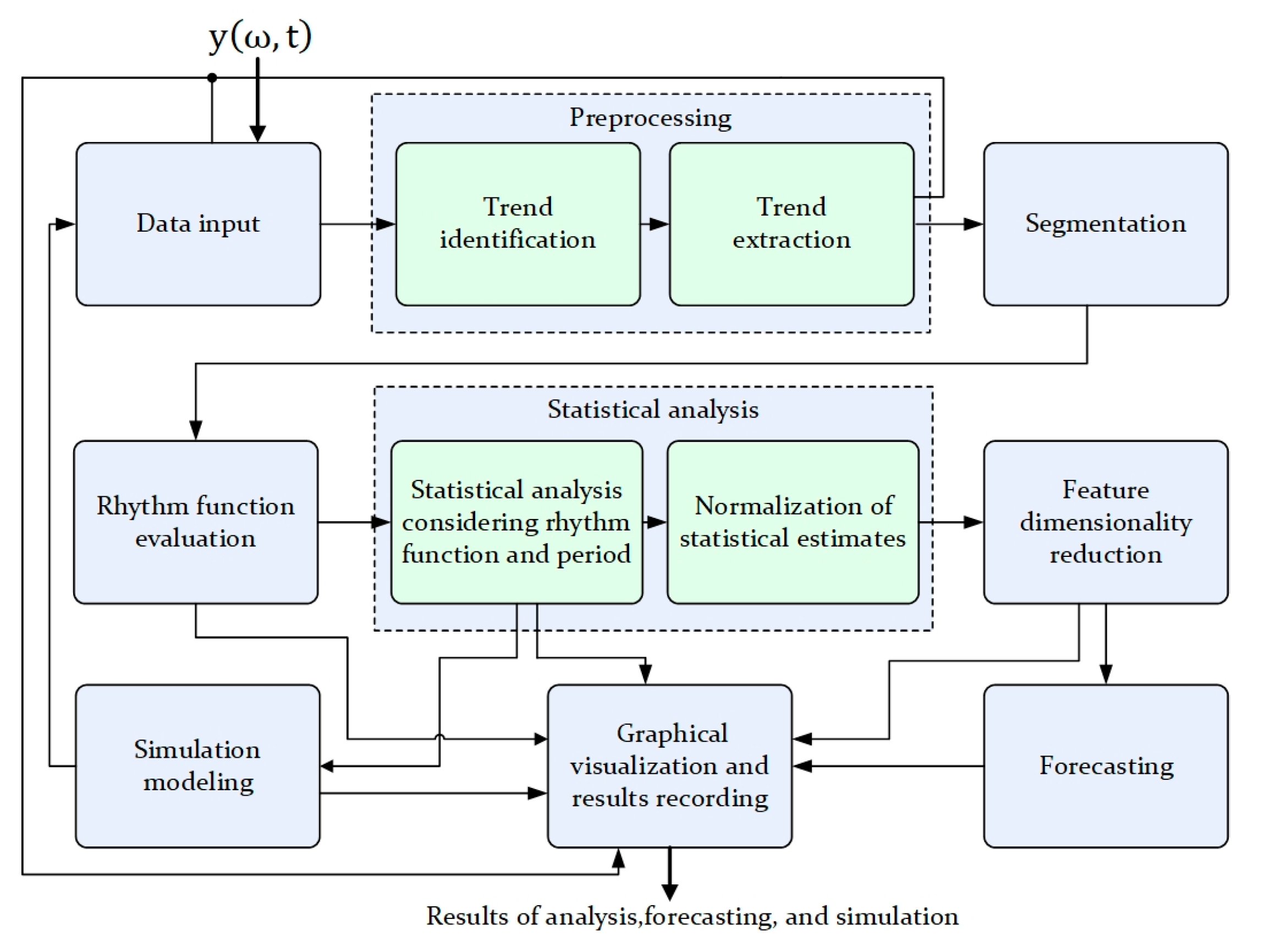
4. The Software System for Modeling, Analysis, and Forecasting of Cyclical Economic Processes as a Component of a Decision Support System

Based on the mathematical model and rhythm-adaptive methods developed above, a software system for modeling, analysis, and forecasting of cyclical economic processes was developed. The software system is implemented in Python (ver. 3.12.0) using the following libraries: Numpy, Pandas, Matplotlib, Seaborn, SciPy. The structural diagram of the software system for modeling, analysis, and forecasting of cyclical economic processes is illustrated in Figure 2.

Let us consider in more detail the functions of the relevant blocks of the software system for the modeling, analysis and forecasting of cyclical economic processes. Subsystem “Data Input” makes it possible to download the implementation of cyclical economic processes to solve the problem of analysis and forecasting, as well as to download estimates of rhythm functions and estimates of probabilistic characteristics of cyclical components to solve problems of computer simulation of cyclical economic processes, as well as testing their processing methods. The subsystem “Evaluation and extraction of trend components” enables evaluation of coefficients $c_j$ of the trend component of the economic process by the method of least squares and separates the deterministic trend and stochastic cyclic components of the economic process under study. The subsystem “Segmentation” makes it possible to segment the cyclical economic process into cycles, as well as to determine a more detailed zonal structure within each of its cycles, which is the basis for evaluating the rhythm function of the cyclical economic process. This subsystem has software tools for manual segmentation by an expert and tools for automated segmentation based on threshold methods and using difference functions of the first and second order. The subsystem “Rhythm Function Evaluation” implements the rhythm function evaluation method based on information about the beginnings of cycles and zones of the economic process and using the method of piecewise linear interpolation. The “Statistical Analysis” subsystem implements a rhythm-adaptive statistical evaluation of the probabilistic characteristics (mathematical expectation, variance and autocorrelation and autocovariance functions, distribution density function) of the cyclical component of the economic process. Also, this subsystem can process economic processes without rhythm adaptation. The subsystem “Feature Dimensionality Reduction” based on Fourier analysis makes it possible to estimate the one-dimensional spectrum of mathematical expectation and the two-dimensional spectrum of the autocorrelation function of the cyclical component of the economic process. On the basis of Bessel’s inequality, the reduction in spectral components and the formation of a vector of informative features for the cyclical component of the economic process are carried out in this subsystem. The subsystem “Forecasting” performs forecasting of the cyclical economic process and the cyclical component based on a new model in the form of the sum of a cyclic random process and a trend function, as well as on the basis of a mathematical model in the form of a sum of a periodic random process and a trend function. The subsystem “Simulation Modeling” allows computer simulation of cyclical economic processes with an arbitrary rhythm function and arbitrary probabilistic characteristics of the cyclic component, as well as with an arbitrary trend component. The “Graphic visualization and results recording” subsystem enables the visualization of all input, intermediate and final results of analysis, forecasting and computer simulation of cyclic economic processes.

5. Experimental Part

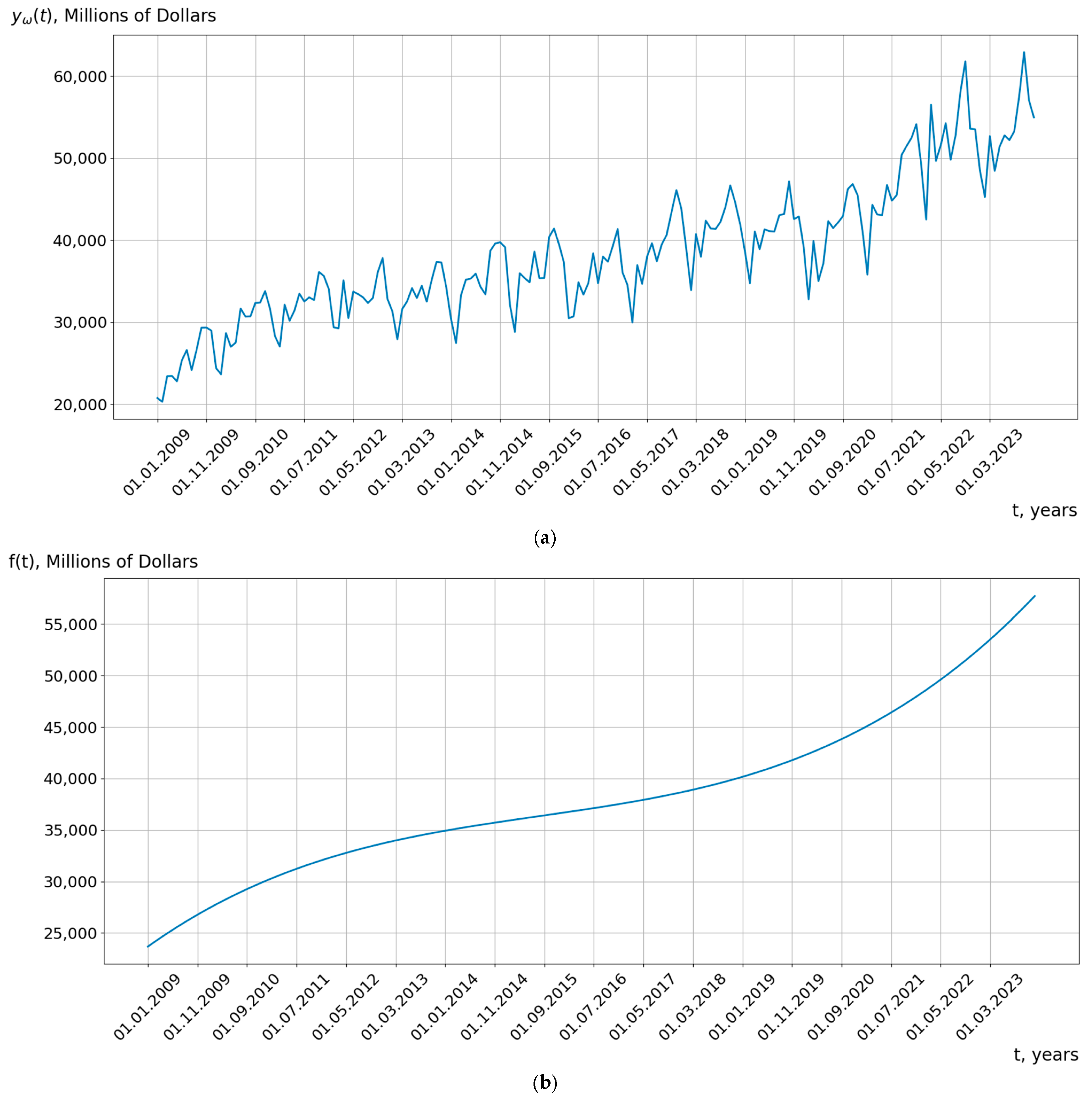
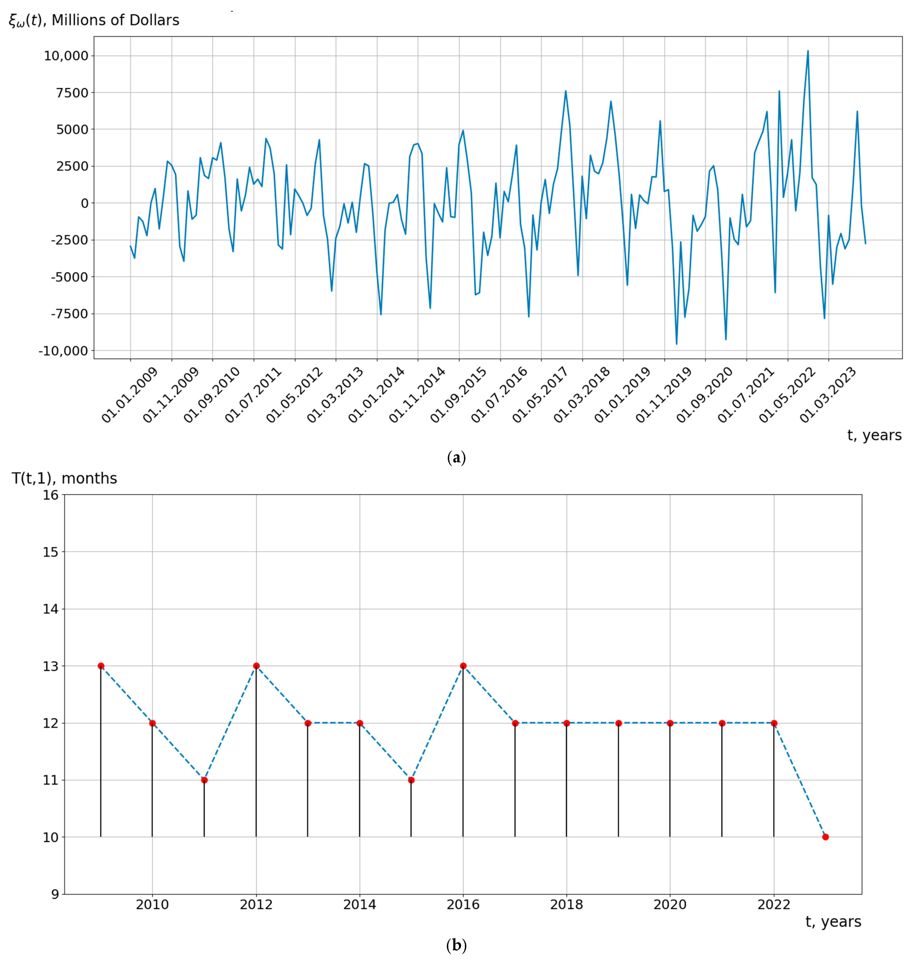
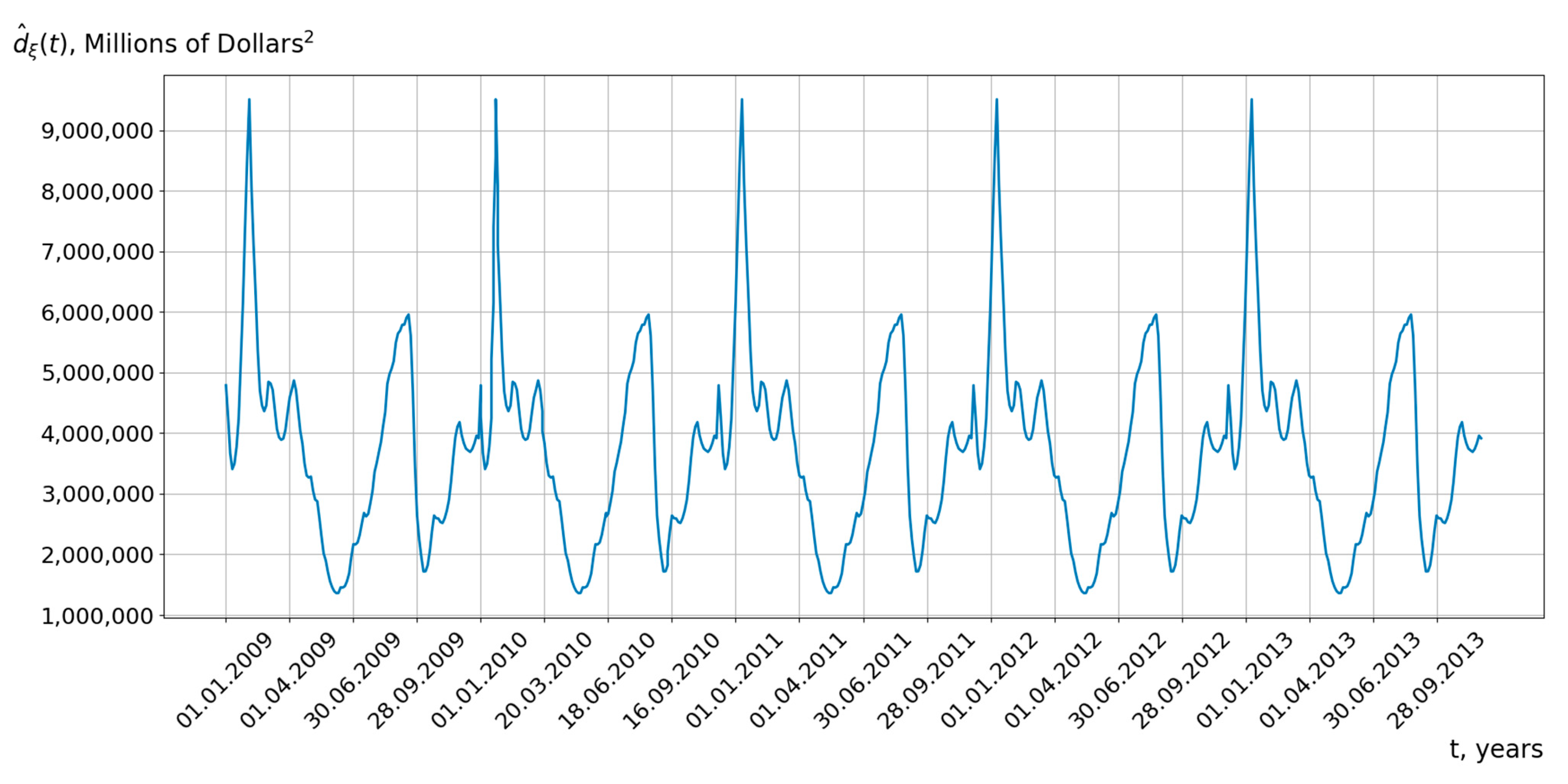
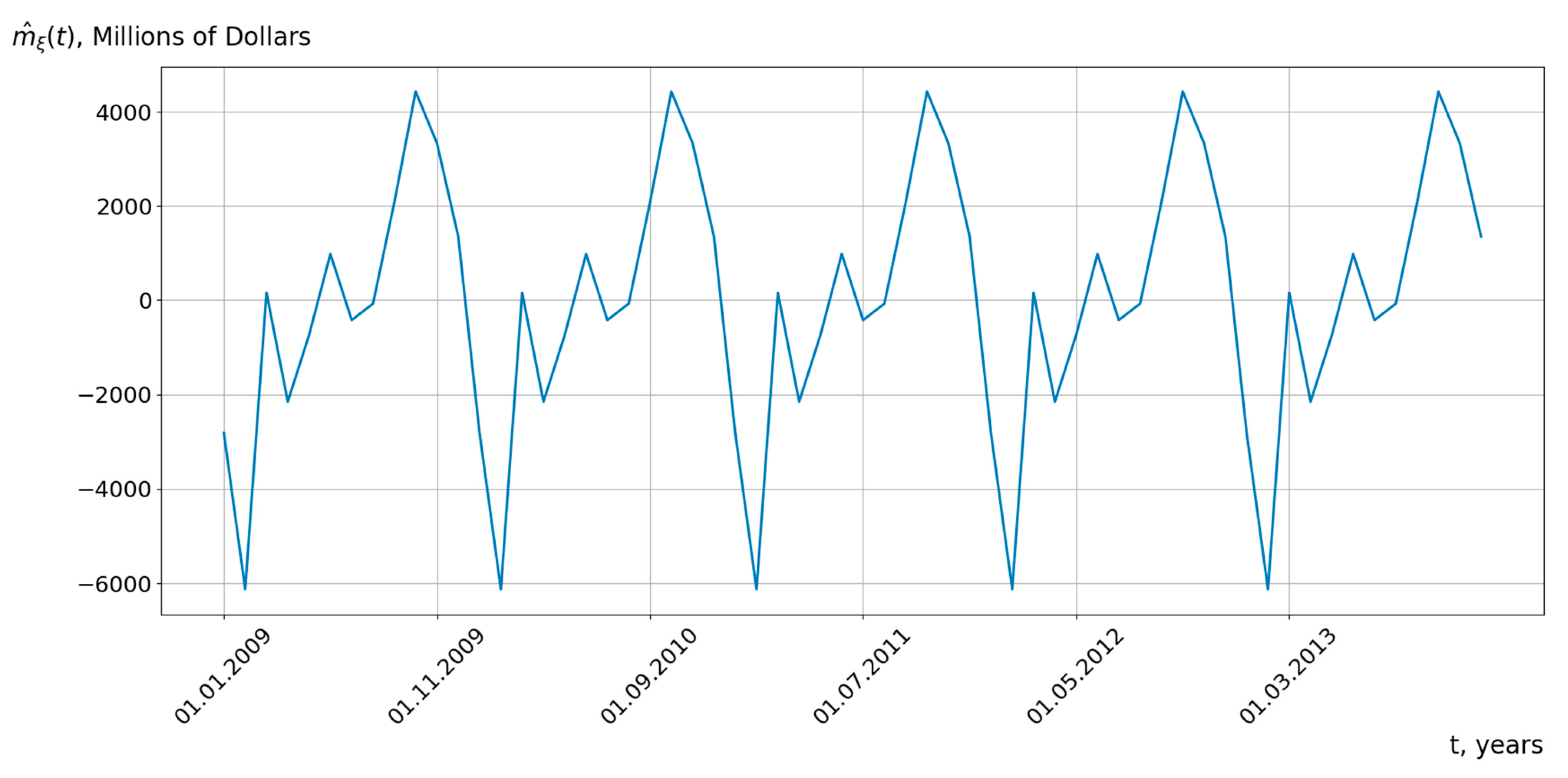
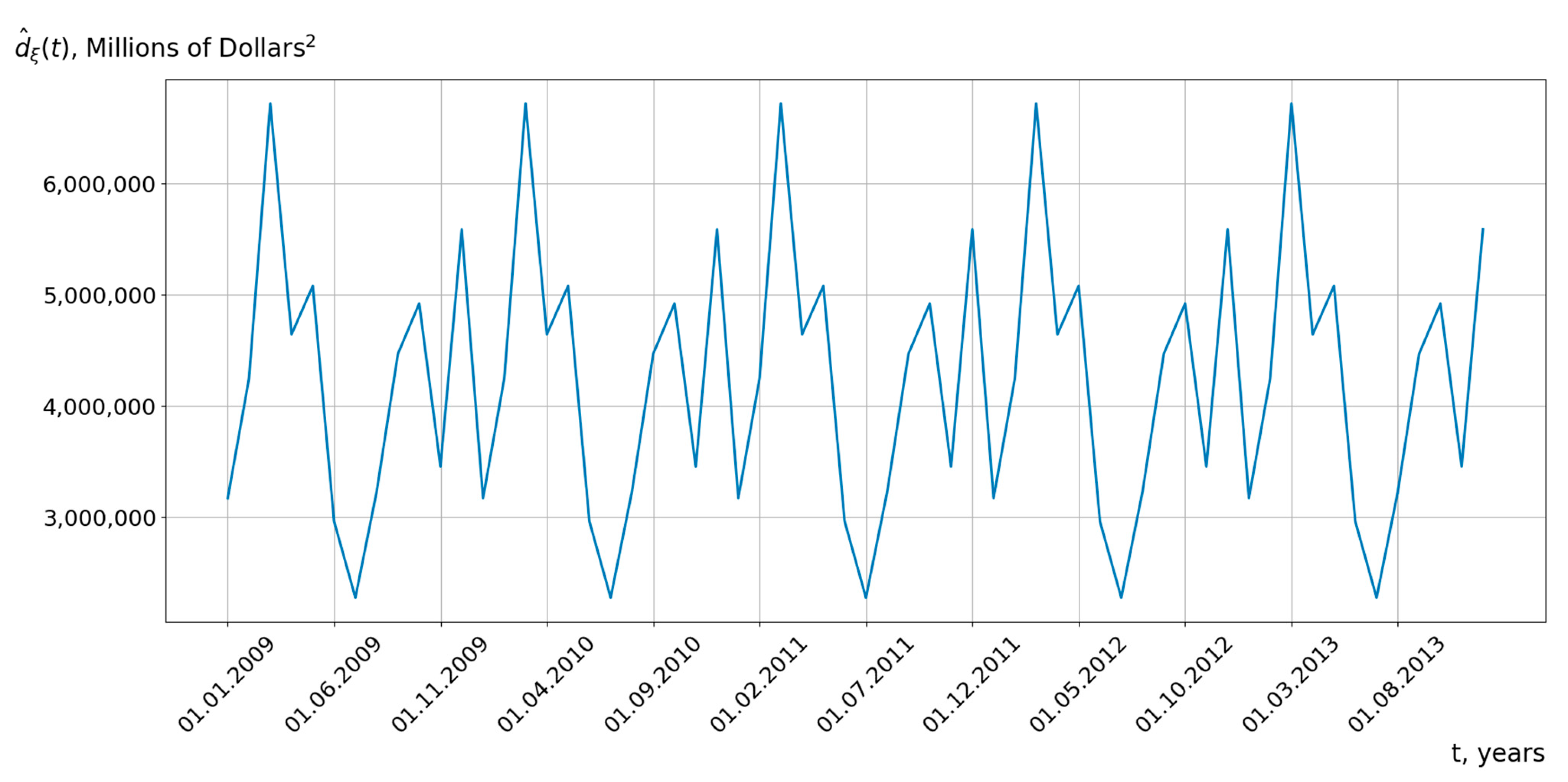
5.1. Results of the Analysis of Cyclical Economic Processes

In order to test the developed mathematical model and methods of processing cyclical economic processes, a series of computational experiments was conducted. Cyclic economic processes were extracted from the Federal Reserve Economic Data database (https://fred.stlouisfed.org/, accessed on 10 January 2025) for further analysis.

Figure 3 shows the cyclic economic process and the estimation of its trend component.

In this study, the linear trend of an economic indicator was assessed using the least squares method. The resulting model is described by the equation $f\left(t\right)=-\mathrm{3,454,126.63}+1731.96\cdot t$, indicating a steady increase in the indicator at an average rate of approximately 1732 units per year. The coefficient of determination $R^2=0.789$ suggests that 78.9% of the variation in values is explained by the linear trend; however, residual fluctuations may indicate the presence of additional influencing factors.

Analysis of the graph reveals that while the overall trend demonstrates an upward trajectory, the actual values exhibit dispersion around the trend line, which may be attributed to seasonal or cyclical effects. This highlights the potential for employing more sophisticated models, such as polynomial regression, exponential smoothing, or seasonal decomposition of time series (STL), to enhance forecasting accuracy. Therefore, the derived model effectively captures the long-term trend of the economic indicator.

Figure 4 shows the cyclical component of the economic process, which is obtained by the formula $\xi \left(\omega ,t\right)=y\left(\omega ,t\right)-f\left(t\right),\omega \in \mathit{\Omega },t\in \mathit{W}$ and piecewise linear estimation of its rhythm function.

Figure 5, Figure 6, Figure 7, Figure 8 and Figure 9 show the rhythm adaptive estimates of mathematical expectation ${\widehat{m}}_{\xi }(t)$, dispersion ${\widehat{d}}_{\xi }(t)$ and the autocorrelation function of the cyclical economic process.

An important issue is the study of the one-dimensional distribution function of cyclical economic processes.

Based on the developed mathematical model and methods for statistical analysis of cyclical economic processes, diagnostic and prognostic features have been substantiated, reflecting the current state and future trends in the development of the economic system represented by the respective cyclical economic processes. This approach has enabled the minimization of volume and maximization of informativeness for diagnostic and prognostic features used for the evaluation, and forecasting of cyclical economic processes in decision support information systems. Specifically, by applying the ${\chi }^2$ goodness-of-fit test with a confidence level of 0.95, the consistency of the investigated cyclical economic processes with the normal distribution law was established (Figure 10).

Considering the established consistency of the distribution of cyclical economic processes with the normal distribution law, it is justified to analyze these economic processes exclusively within the framework of the first two moment functions.

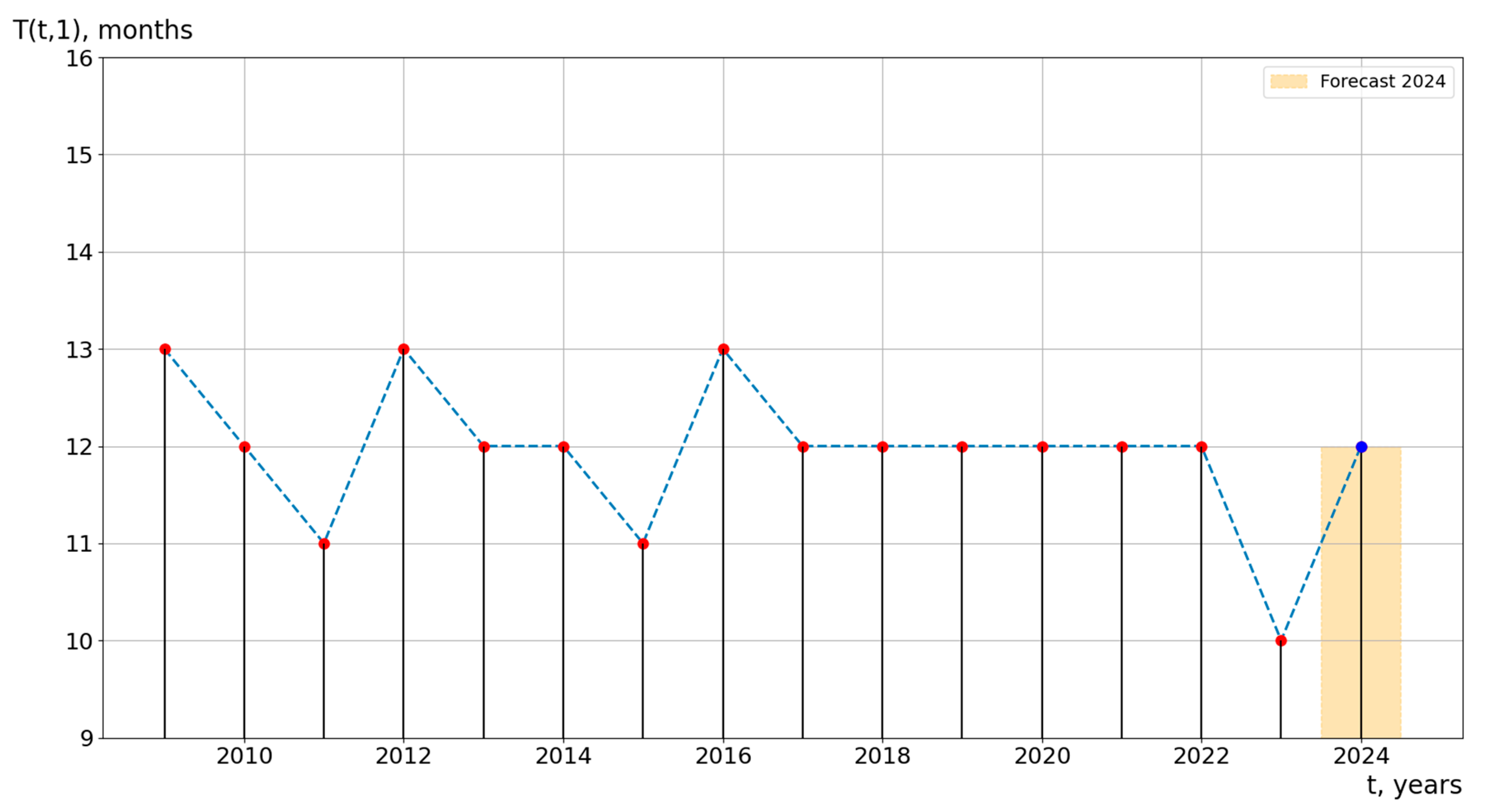
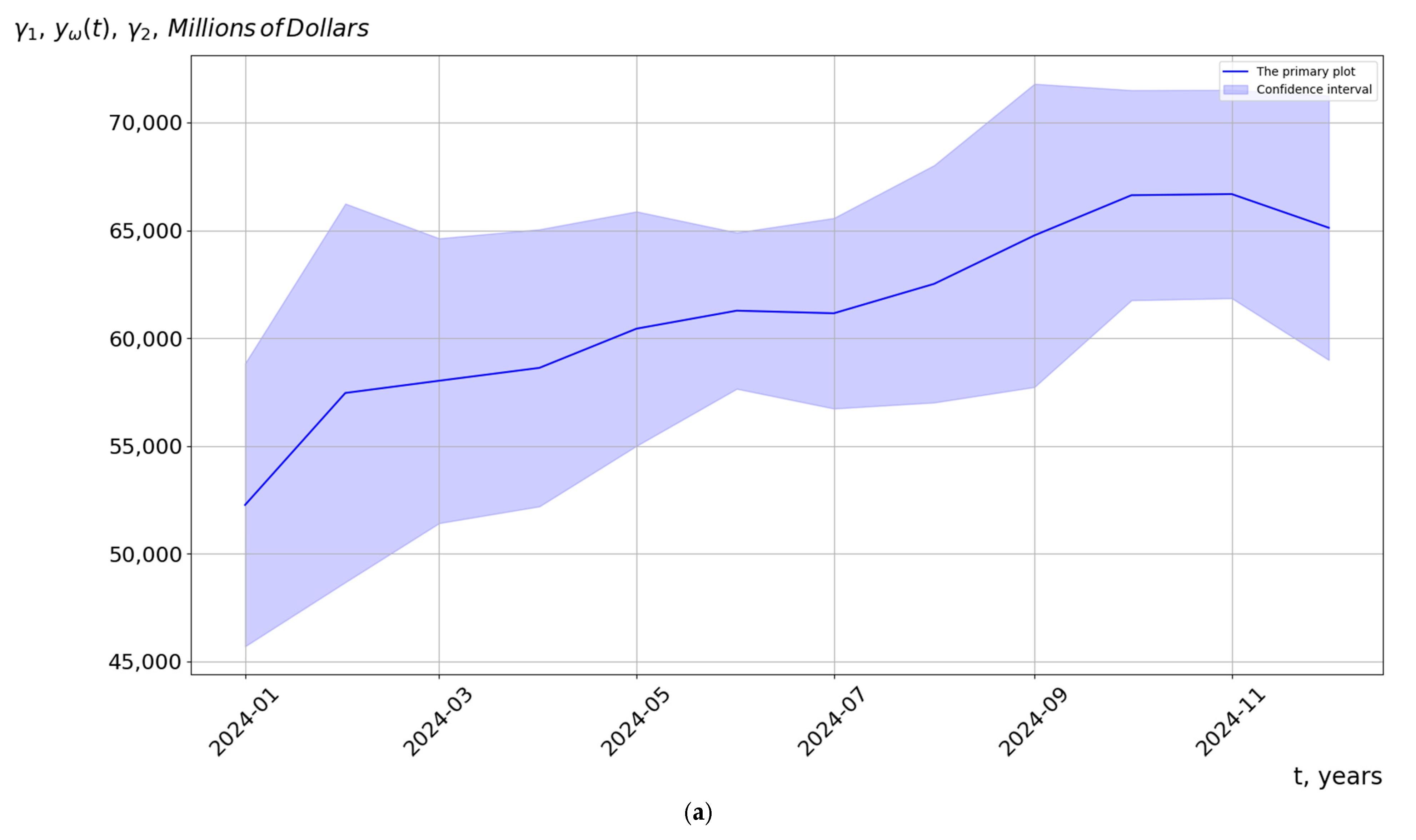
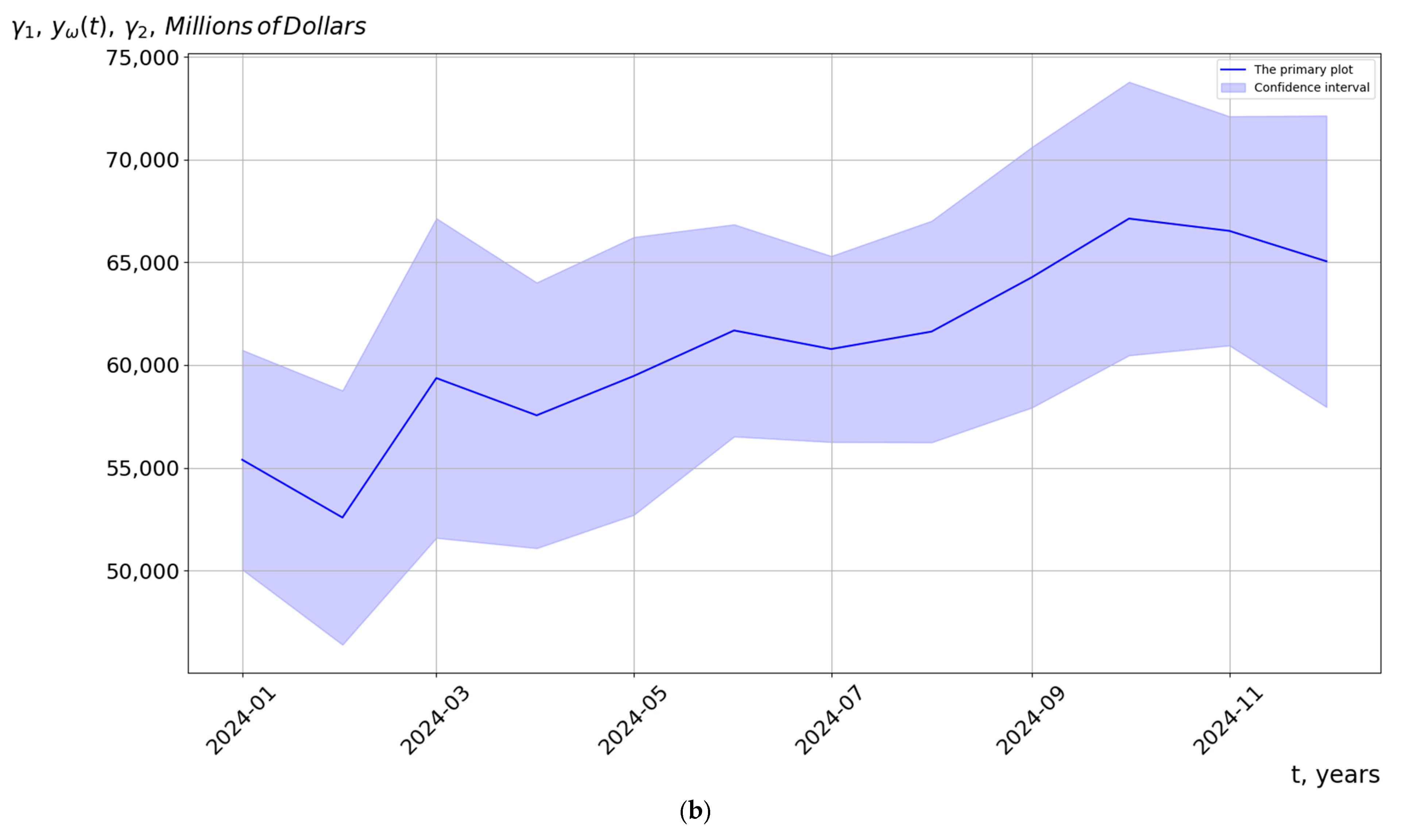
5.2. Results of Forecasting of Cyclical Economic Processes

Based on the received statistical estimates of the mathematical expectation and dispersion of the cyclical component of the economic process, we will forecast its next cycle. For this purpose, we forecast the duration of the future cycle of the economic process. For example, based on the known values of the rhythm function of the cyclical component of the economic series U.S. Imports of Goods by Customs Basis from Advance Technology Products, its projected value for 2024 was estimated as the average of the previous values (the result is presented in Figure 11).

Taking into account the rhythm function along with its predicted value for 2024 (Figure 11), as well as the estimates of the mathematical expectation and variance (see Figure 5, Figure 6, Figure 7 and Figure 8), confidence intervals $\Upsilon \in \left[{\gamma }_1\right(t),{\gamma }_2(t\left)\right]$ were constructed in Figure 12 based on models in the form of a cyclical random process and a periodic random process. For the latter model, the period value is $T=12$.

Table 2. Comparison of the mean absolute error in forecasting the economic series of U.S. Imports of Goods by Customs Basis from Advance Technology Products for 2024, based on mathematical models in the form of a cyclical random process and a periodic random process, with a confidence level of 0.95.

A Forecasting Method Based on a Model in the Form of a Cyclical Random Process.	A Forecasting Method Based on a Model in the Form of a Periodic Random Process.
${\mathit{z}}_{{\mathit{k}}_{\mathit{\xi }}}=$ 2925.72 Million USD	${\mathit{z}}_{{\mathit{k}}_{\mathit{\xi }}}^{\mathit{’}}=$ 6105.54 Million USD

where ${\mathit{z}}_{{\mathit{k}}_{\mathit{\xi }}}$ is the absolute forecasting error averaged over a cycle when using a forecasting method based on a model in the form of a cyclical random process; ${\mathit{z}}_{{\mathit{k}}_{\mathit{\xi }}}^{\mathit{’}}$ is the absolute forecasting error averaged over a cycle when using a forecasting method based on a model in the form of a periodic random process.

presents the results of comparing the mean absolute error in forecasting a cyclical economic process based on its new and existing models.

Comparing the mean absolute errors (Table 2), it was established that the forecasting method for cyclical economic processes based on the new model, represented as the sum of a deterministic polynomial function and a cyclical random process, provides higher forecasting accuracy compared to the method based on the known model, represented as the sum of a deterministic trend function and a periodic random process. As a result of the conducted series of forecasting experiments, it was determined that the forecasting accuracy improved by 52% on average.

6. Discussion and Conclusions

As part of this research, a comparison of forecasting results was conducted between the new model based on a cyclical random process and the known model based on a periodic random process. The experiments demonstrated that the model based on a cyclical random process provides better forecasting results compared to the known model based on a periodic random process. Future work will focus on improving the forecasting accuracy of the results.

The main conclusions of the study:

• Based on the results of a comprehensive review of the literature, a comparative analysis of existing mathematical models, methods, and software tools for the analysis and forecasting of cyclical economic processes was conducted. This analysis identified a number of shortcomings and outlined the direction for further research.
• A new mathematical model of cyclical economic processes was developed, represented as the sum of a deterministic polynomial function and a cyclical random process. By incorporating trend components, stochasticity, cyclicality, and rhythm variability of cyclical economic processes, this model improved the accuracy, reliability, and informativeness of methods and software tools for their modeling, analysis, and forecasting.
• A new statistical method for processing (analysis and forecasting) cyclical economic processes was substantiated, characterized by enhanced accuracy in estimating probabilistic characteristics of the studied processes through its adaptation to changes in their rhythm.

In subsequent articles, we plan to describe methods of simulation modeling based on the cyclical random process model and present the simulation results with an evaluation of simulation accuracy. The software component of the research will also be elaborated in more detail in upcoming scientific papers.

References

1. Hodrick, R.J. An Exploration of Trend-Cycle Decomposition Methodologies in Simulated Data National Bureau of Economic Research. NBER Working Paper 26750. 2020. Available online: http://www.nber.org/papers/w26750.pdf (accessed on 10 January 2025).
2. Kang, N.; Marmer, V. Modeling long cycles. J. Econ. Dyn. Control 2024, 5, 120–163. [Google Scholar] [CrossRef]
3. Lenart, Ł.; Kwiatkowski, Ł.; Wróblewska, J. A Bayesian nonlinear stationary model with multiple frequencies for business cycle analysis. arXiv 2024, arXiv:2406.02321. [Google Scholar]
4. Krüger, J.J. A wavelet evaluation of some leading business cycle indicators for the German economy. J. Bus. Cycle Res. 2021, 17, 293–319. [Google Scholar] [CrossRef]
5. Guvenen, F.; McKay, A.; Ryan, C. A Tractable Income Process for Business Cycle Analysis; National Bureau of Economic Research, Inc.: Cambridge, MA, USA, 2023. [Google Scholar]
6. Wildi, M. Business-cycle analysis and zero-crossings of time series: A generalized forecast approach. J. Bus. Cycle Res. 2024, 20, 155–192. [Google Scholar] [CrossRef]
7. Bernard, L.; Gevorkyan, A.; Palley, T.; Semmler, W. Long-wave economic cycles: The contributions of Kondratieff, Kuznets, Schumpeter, Kalecki, Goodwin, Kaldor, and Minsky. J. Econ. Dyn. Struct. 2024, 5, 120–163. [Google Scholar]
8. Pontes, E.L.; Benjannet, M.; Yung, R. Forecasting Four Business Cycle Phases Using Machine Learning: A Case Study of US and EuroZone. arXiv 2024, arXiv:2405.17170. [Google Scholar]
9. Azqueta-Gavaldon, A.; Hirschbühl, D.; Onorante, L.; Saiz, L. Nowcasting Business Cycle Turning Points with Stock Networks and Machine Learning; European Central Bank Working Paper Series #2494; European Central Bank: Frankfurt, Germany, 2020. [Google Scholar]
10. Kuntze, V. The Role of Coincident Information in Real-Time Business Cycle Forecasting. SSRN 2024, 4692581. Available online: https://papers.ssrn.com/sol3/papers.cfm?abstract_id=4692581 (accessed on 21 March 2025). [CrossRef]
11. Mariani, M.C.; Bhuiyan, M.A.M.; Tweneboah, O.K.; Beccar-Varela, M.P.; Florescu, I. Analysis of stock market data by using Dynamic Fourier and Wavelets techniques. Phys. A Stat. Mech. Its Appl. 2020, 537, 122785. [Google Scholar] [CrossRef]
12. Pisol, M.; Harun, M.; Abdul Latif, R. Utilization of Holt-Winters Exponential Smoothing Model in Forecasting 2023 LZNK Collection. Int. J. Zakat Islam. Philanthr. 2023, 5, 163–172. [Google Scholar]
13. Tiao, G.C.; Grupe, M.R. Hidden periodic autoregressive-moving average models in time series data. Biom. 1980, 67, 365–373. [Google Scholar] [CrossRef]
14. Todd, R. A Dynamic Equilibrium Model of Seasonal and Cyclical Fluctuations in the Corn–Soybean–Hog Sector; University of Minnesota: Minneapolis, MN, USA, 1983. [Google Scholar]
15. Todd, R. Periodic linear–quadratic methods for modeling seasonality. J. Econ. Dyn. Control 1990, 14, 763–795. [Google Scholar] [CrossRef]
16. Osborn, D.R. Seasonality and habit persistence in a life cycle model of consumption. J. Appl. Econom. 1988, 3, 255–266. [Google Scholar] [CrossRef]
17. Osborn, D.R.; Smith, J.P. The performance of periodic autoregressive models in forecasting seasonal U.K. consumption. J. Bus. Econ. Stat. 1989, 7, 117–128. [Google Scholar] [CrossRef]
18. Hansen, L.P.; Sargent, T.J. Recursive Linear Models of Dynamic Economies; Hoover Institution, Stanford University: Stanford, CA, USA, 1990. [Google Scholar]
19. Chen, L.; Dolado, J.J.; Gonzalo, J.; Pan, H. Estimation of Characteristics-Based Quantile Factor Models (PHBS Working Paper No. 20220701); Peking University HSBC Business School: Beijing, China, 2022. [Google Scholar]
20. Huang, H. Analysis and Forecast of Resource-based City GDP Based on ARIMA Model. Adv. Econ. Bus. Manag. Res. 2019, 76, 210–216. [Google Scholar]
21. Eckert, F.; Hyndman, R.J.; Panagiotelis, A. Forecasting Swiss exports using Bayesian forecast reconciliation. Eur. J. Oper. Res. 2021, 291, 693–710. [Google Scholar] [CrossRef]
22. Choi, H.K. Stock price correlation coefficient prediction with ARIMA-LSTM hybrid model. arXiv 2018, arXiv:1808.01560. [Google Scholar]
23. Krolzig, H.-M. Econometric Modelling of Markov-Switching Vector Autoregressions using MSVAR for Ox (Discussion Paper No. 9802); Nuffield College, University of Oxford: Oxford, UK, 1998. [Google Scholar]
24. Amisano, G.; Colavecchio, R. Money Growth and Inflation: Evidence from a Markov Switching Bayesian VAR (Paper No. 4/2013); Department of Socioeconomics, University of Hamburg: Hamburg, Germany, 2013. [Google Scholar]
25. Shin, M.; Kim, D.; Wang, Y.; Fan, J. Factor and idiosyncratic VAR-Ito volatility models for heavy-tailed high-frequency financial data. arXiv 2023, arXiv:2109.05227. [Google Scholar]
26. Ghysels, E. Are Business Cycle Turning Points Uniformly Distributed Throughout the Year? (Discussion Paper No. 3891); Université de Montréal: Montréal, QC, Canada, 1991. [Google Scholar]
27. Ghysels, E. On the Periodic Structure of the Business Cycle (Discussion Paper No. 1028); Cowles Foundation, Yale University: New Haven, CO, USA, 1992. [Google Scholar]
28. Hamilton, J.D. Rational-expectations econometric analysis of changes in regime: An investigation of the term structure of interest rates. J. Econ. Dyn. Control 1988, 12, 385–423. [Google Scholar] [CrossRef]
29. Hamilton, J.D. A new approach to the economic analysis of nonstationary time series and the business cycle. Econometrica 1989, 57, 357–384. [Google Scholar] [CrossRef]
30. Hamilton, J.D. Analysis of time series subject to changes in regime. J. Econom. 1990, 45, 39–70. [Google Scholar] [CrossRef]
31. Garcia, R.; Perron, P. An analysis of the real interest rate under regime shifts (Unpublished manuscript); Princeton University: Princeton, NJ, USA, 1989. [Google Scholar]
32. Phillips, K.L. A two-country model of stochastic output with changes in regime. J. Int. Econ. 1991, 31, 121–142. [Google Scholar] [CrossRef]
33. McCulloch, R.E.; Tsay, R.S. Statistical inference of Markov switching models with applications to US GNP (Technical Report No. 125); Graduate School of Business, University of Chicago: Chicago, IL, USA, 1992. [Google Scholar]
34. Albert, J.; Chib, S. Bayes inference via Gibbs sampling of autoregressive time series subject to Markov mean and variance shifts. J. Bus. Econ. Stat. 1993, 11, 1–15. [Google Scholar] [CrossRef]
35. McCracken, M.W.; Owyang, M.T.; Sekhposyan, T. Real-time forecasting and scenario analysis using a large mixed-frequency Bayesian VAR. Int. J. Cent. Bank. 2021, 18, 327–355. [Google Scholar]
36. Alsinglawi, O.; Aladwan, M.; Alwadi, S.; Alazzam, E. Forecasting Economic Growth and Movements with Wavelet Transform and ARIMA Model. Appl. Math. Inf. Sci. 2023, 17, 817–828. [Google Scholar]
37. Vîntu, D. GDP modelling and forecasting using ARIMA: An empirical assessment for innovative economy formation. Eur. J. Econ. Stud. 2021, 10, 29–44. [Google Scholar] [CrossRef]
38. Petrova, A.; Deyneka, M. ARIMA-models: Modeling and forecasting prices of stocks. Int. Sci. J. “Internauka” 2022, 2, 1–19. [Google Scholar] [CrossRef]
39. Ma, Y. Analysis and Forecasting of GDP Using the ARIMA Model. Inf. Syst. Econ. 2024, 5, 91–97. [Google Scholar]
40. Lai, H.; Ng, E. On business cycle forecasting. Front. Bus. Res. China 2020, 14, 17. [Google Scholar] [CrossRef]
41. Tran, T.N. The Volatility of the Stock Market and Financial Cycle: GARCH Family Models. J. Ekon. Malays. 2022, 56, 151–168. [Google Scholar]
42. Ng, P.; Kwok, M.; Cheng, C. Business Cycle and Early Warning Indicators for the Economy of Hong Kong—Challenges of Forecasting Work amid the COVID-19 Pandemic. J. Bus. Cycle Res. 2024, 20, 123–135. [Google Scholar] [CrossRef]
43. Rekova, N.; Telnova, H.; Kachur, O.; Holubkova, I.; Balezentis, T.; Streimikiene, D. Financial sustainability evaluation and forecasting using the Markov chain: The case of the wine business. Sustainability 2020, 12, 6150. [Google Scholar] [CrossRef]
44. Lin, Y.; Sung, B.; Park, S. Integrated systematic framework for forecasting China’s consumer confidence: A machine learning approach. Systems 2024, 12, 445. [Google Scholar] [CrossRef]
45. Tang, P.; Zhang, Y. China’s business cycle forecasting: A machine learning approach. Comput. Econ. 2024, 64, 2783–2811. [Google Scholar] [CrossRef]
46. Masini, R.; Medeiros, M.; Mendes, E. Machine Learning Advances for Time Series Forecasting. J. Econ. Surv. 2023, 37, 76–111. [Google Scholar] [CrossRef]
47. Sako, K.; Mpinda, B.; Rodrigues, P. Neural Networks for Financial Time Series Forecasting. Entropy 2022, 24, 657. [Google Scholar] [CrossRef]
48. Wang, Y.; Lin, T. A novel deterministic probabilistic forecasting framework for gold price with a new pandemic index based on quantile regression deep learning and multi-objective optimization. Mathematics 2024, 12, 29. [Google Scholar] [CrossRef]
49. Arslan, M.; Hunjra, A.; Ahmed, W.; Zaied, Y. Forecasting multi-frequency intraday exchange rates using deep learning models. J. Forecast. 2024, 43, 1338–1355. [Google Scholar] [CrossRef]
50. Kinlaw, W.; Kritzman, M.; Turkington, D. A new index of the business cycle. J. Invest. Manag. 2021, 19, 4–19. [Google Scholar] [CrossRef]
51. Rademacher, P. Forecasting Recessions in Germany with Machine Learning; DICE Discussion Paper #416; Heinrich Heine University Düsseldorf, Düsseldorf Institute for Competition Economics (DICE): Düsseldorf, Germany, 2024. [Google Scholar]
52. Chaiboonsri, C.; Wannapan, S. Big data and machine learning for economic cycle prediction: Application of Thailand’s economy. Lect. Notes Artif. Intell. 2020, 11471, 347–359. [Google Scholar]
53. Garg, R.; Sah, A. Cyclical dynamics and co-movement of business, credit, and investment cycles: Empirical evidence from India. Humanit. Soc. Sci. Commun. 2024, 11, 515. [Google Scholar] [CrossRef]
54. Chai, S.; Lim, J.; Yoon, H.; Wang, B. A novel methodology for forecasting business cycles using ARIMA and neural network with weighted fuzzy membership functions. Axioms 2024, 13, 56. [Google Scholar] [CrossRef]
55. Benrhmach, G.; Namir, K.; Bouyaghroumni, J.; Namir, A. Financial Time Series Prediction Using Wavelet and Artificial Neural Network. J. Math. Comput. Sci. 2021, 11, 5487–5500. [Google Scholar]
56. Leventides, J.; Melas, E.; Poulios, C. Extended dynamic mode decomposition for cyclic macroeconomic data. Data Sci. Financ. Econ. 2022, 2, 117–146. [Google Scholar] [CrossRef]
57. Lupenko, S. Rhythm-adaptive statistical estimation methods of probabilistic characteristics of cyclic random processes. Digit. Signal Process. 2024, 151, 104563. [Google Scholar] [CrossRef]
58. Lupenko, S. Abstract Cyclic Functional Relation and Taxonomies of Cyclic Signals Mathematical Models: Construction, Definitions and Properties. Mathematics 2024, 12, 3084. [Google Scholar] [CrossRef]
59. Lupenko, S. The rhythm-adaptive Fourier series decompositions of cyclic numerical functions and one-dimensional probabilistic characteristics of cyclic random processes. Digit. Signal Process. 2023, 140, 104104. [Google Scholar] [CrossRef]
60. Lupenko, S.; Butsiy, R.; Shakhovska, N. Advanced Modeling and Signal Processing Methods in Brain–Computer Interfaces Based on a Vector of Cyclic Rhythmically Connected Random Processes. Sensors 2023, 23, 760. [Google Scholar] [CrossRef]
61. Lupenko, S.; Butsiy, R. Isomorphic Multidimensional Structures of the Cyclic Random Process in Problems of Modeling Cyclic Signals with Regular and Irregular Rhythms. Fractal Fract. 2024, 8, 203. [Google Scholar] [CrossRef]
62. Lupenko, S. The Mathematical Model of Cyclic Signals in Dynamic Systems as a Cyclically Correlated Random Process. Mathematics 2022, 10, 3406. [Google Scholar] [CrossRef]
Figure 1. Examples of graphs of realizations of typical cyclic economic processes: U.S. Imports of Goods by Customs Basis from Advance Technology Products (a), Unemployment Rate—Agricultural and Related Private Wage and Salary Workers (b), Unemployment Rate—16–19 Yrs. (c), Unemployment Rate—Farming, Fishing, and Forestry Occupations (d).
Forecasting 07 00020 g001aForecasting 07 00020 g001b
Figure 2. Structural Diagram of a Software System for Modeling, Analysis, and Forecasting of Cyclical Economic Processes.
Forecasting 07 00020 g002
Figure 3. U.S. Imports of Goods by Customs Basis from Advance Technology Products: (a) realization of cyclical economic process; (b) trend component.
Forecasting 07 00020 g003
Figure 4. U.S. Imports of Goods by Customs Basis from Advance Technology Products: (a) cyclic component; (b) rhythm function (interpolated rhythm function is indicated by dashed line).
Forecasting 07 00020 g004
Figure 5. Estimation of the mathematical expectation based on a model in the form of cyclic random processes of U.S. Imports of Goods by Customs Basis from Advance Technology Products.
Forecasting 07 00020 g005
Figure 6. Estimation of the dispersion based on a model in the form of cyclic random process of U.S. Imports of Goods by Customs Basis from Advance Technology Products.
Forecasting 07 00020 g006
Figure 7. Estimation of the mathematical expectation based on a model in the form of periodic random process of U.S. Imports of Goods by Customs Basis from Advance Technology Products.
Forecasting 07 00020 g007
Figure 8. Estimation of the dispersion based on a model in the form of periodic random process of U.S. Imports of Goods by Customs Basis from Advance Technology Products.
Forecasting 07 00020 g008
Figure 9. Realizations of statistical estimates of autocorrelation functions of U.S. Imports of Goods by Customs Basis from Advance Technology Products based on processing using a model in a form of: a cyclical random process (a) and a periodic random process (b).
Forecasting 07 00020 g009
Figure 10. A cross-section plot of the realization of the estimated one-dimensional probability density function of U.S. Imports of Goods by Customs Basis from Advance Technology Products.
Forecasting 07 00020 g010
Figure 11. The rhythm function of the economic series U.S. Imports of Goods by Customs Basis from Advance Technology Products with a forecasted value for the year 2024.
Forecasting 07 00020 g011
Figure 12. Confidence intervals for U.S. Imports of Goods by Customs Basis from Advance Technology Products for 2024, based on mathematical models in the form of: (a) a cyclical random process and (b) a periodic random process.
Forecasting 07 00020 g012aForecasting 07 00020 g012b