Abstract
The fresh produce supply chain sector is a vital pillar of any society and an indispensable part of the national economic structure. As a significant segment of the agricultural market, accurately forecasting vegetable prices holds significant importance. Vegetable market pricing is subject to a myriad of complex influences, resulting in nonlinear patterns that conventional time series methodologies often struggle to decode. Future planning for commodity pricing is achievable by forecasting the future price anticipated by the current circumstances. This paper presents a price forecasting methodology for tomatoes which uses price and production data taken from 2008 to 2021 and analyzed by means of advanced deep learning-based Long Short-Term Memory (LSTM) networks. A comparative analysis of three models based on Root Mean Square Error (RMSE) identifies LSTM as the most accurate model, achieving the lowest RMSE (0.2818), while SARIMA performs relatively well. The proposed deep learning-based method significantly improved the results versus other conventional machine learning and statistical time series analysis methods.
1. Introduction
Agricultural price prediction has become a critical anchor to food security, food waste reduction, and sustainability [1,2]. Important market players such as producers, processors, consumers, hedgers, and policymakers depend on accurate forecasts of agricultural produce to engage effectively with the market, as well as to ensure better supply chain management [3,4]. Vegetables, in particular, are great sources of nutrients and form a vital part of the human daily diet while significantly contributing to local and national agricultural economies [3,5]. The fresh produce market (FPM), which is an important key player in the South African economy, manages the daily operations of the sector. The FPM ensures that a smooth transition of agricultural produce (from farm to fork) is achieved daily. However, the FPM is faced with many challenges, ranging from poor returns to low purchases and food waste [6,7].
Price and demand fluctuations have been identified as one of the leading causes of poor economic returns. This is purely due to the nature of agricultural commodity prices. Among other variables that predispose agricultural prices to volatility and sharp changes in and around one calendar year is seasonality [8]. Other factors include climate change, political influence, and supply-and-demand relationships, among others [9].
Tomato (Solanum Lycopersicon) makes up one of the most utilized vegetables in the world and is only behind potato in global importance [10]. In South Africa, the tomato industry contributes about 18.3% to the gross value of vegetable production [11]. Now, tomato distribution is achieved through four major channels, namely, the national fresh produce markets (FPMs), exports, processing, and direct marketing [12]. The Cape Town fresh produce market (CFPM) is South Africa’s third major center for the marketing of fresh produce after the Johannesburg and Tshwane FPMs and controls about 12% of the market share of the total NFPMs [12]. Currently, production sits at 487000 T for the 2022/2023 season, which is a decline from the previous production value of 534000 T in 2021/2022 [11,13], hence indicating consistent and irregular changes in production, sales, and price values, adding to other environmental factors and dynamics.
1.1. Research Rationale
The tomato value chain is plagued with increased fluctuating retail pricing [13], among other challenges. Stakeholders, including producers, processors, national fresh produce markets, exporters, retailers, wholesalers, and consumers, now seek innovative ways to address this crisis.
Accurate price prediction/forecasting is critical for any viable economic enterprise. Poor pricing leads to poor wholesale or fresh produce market management, which consequently leads to food waste, as excessive supply could outweigh demand. It is reported that over 40% of fresh fruits and vegetables (FFVs) is lost due to waste. In South Africa, studies estimate that losses can be between 13.5 and 19% of total production [13,14,15].
Consequently, it becomes imperative that a timely and highly accurate price forecasting approach be introduced to attempt to address these fluctuations and poor decision making on the part of the different stakeholders in the industry.
Existing methods for agricultural price forecasting include econometric approaches (e.g., ARIMA, SARIMA), traditional machine learning algorithms (Support Vector Regression (SVR), Random Forest (RF), K-nearest neighbors (k-NN), Extreme Gradient Boosting (XGB)), and emerging deep learning (DL) methods (Artificial Neural Networks (ANNs), Long Short-Term Memory (LSTM), Convolutional Neural Networks (CNN), Gated Recurrent Units (GRUs), Gaussian process (GP) regression, etc.) [1,16,17,18]. Recently, DL-based methods have significantly influenced forecasting research, demonstrating strong potential in predicting and modeling time series data [1,2,3,4,5,6,7,8,9,10,11,12,13,14,15,16,17,18,19].
In the past decade, numerous studies have successfully applied deep learning models, particularly LSTM, for agricultural price forecasting [1,20,21], with LSTM proving very effective for agricultural price forecasting analysis. These methods address the limitations of traditional approaches in managing nonlinear, nonstationary, and dynamically varying time series data. DL models can uncover deeper insights compared to classical machine learning and econometric methods. However, DL methodologies present notable challenges, including model training complexities, parameter tuning and optimization difficulties, and issues concerning model architecture design and practical implementation.
In this study, we aim to evaluate the effectiveness of the deep learning-based LSTM method in accurately modeling price variations and forecasting future prices. We explore and compare the performance of four additional forecasting models—ARIMA, SARIMA, SVR, and XGB—against the LSTM approach.
1.2. Related Work
Agricultural product (fresh produce) prices undergo frequent fluctuations over periodic intervals. Although research suggests that demand and supply exert the highest influence on prices, the prices of agricultural produce are also influenced by other factors, including production, weather changes, policy interventions, and market risks, among others [5]. Nevertheless, the prices of commodities often show irregular, nonlinear, and dynamic trends when analyzed [1,5]. These uncertainties in the relationship between prices and various independent variables make the analysis of these trends difficult [8].
Several authors have attempted to explore different approaches to analyzing price trends and to develop prediction and forecasting models for different types of fresh agricultural produce [1]. Zhang et al. [3] collected daily prices of fresh produce (vegetables) between 2009 and 2023 from wholesale markets in Beijing and developed prediction models for future prices using four different models. The authors compared their performance and found that LSTM outperformed the other models. LSTM achieved over 5% improvement compared to the conventional approaches, thus proving to be effective in decoding delicate time series datasets. A similar price forecasting study was conducted by other experts [5]. The authors evaluated different models and provided the relative advantage of one approach over another. The large learning model-based method was found to outperform all the other forecasting methods. Several other deep learning-based approaches involving vegetable price prediction have also been reported [20,22,23]. Although they used different models for vegetable price prediction, these studies reported relatively accurate prediction performance.
In a price forecasting study on strawberry fruit, Okwuchi [24] explored several deep learning-based approaches and compared their performance. The authors modeled their time series predictions using both daily and weekly data on the weather and on the yield, prices, and sales of strawberries. DL-based methods showed better performance. However, the authors observed that the use of attention mechanisms significantly improved model performance. A similar study on strawberry prices also reported the effectiveness of DL-based methods for time series prediction purposes [23]. Other studies involving DL-based approaches for price forecasting analysis of fresh produce samples include RNN for banana [25] and LSTM for soybean [26], millet, sorghum, and maize [27], rapeseed [28], and strawberries [29]. A summary of the different applications of deep learning-based methods is provided in Table 1.

Table 1.
Summary of different applications of ML- and DL-based approaches for price forecasting and prediction for fresh agricultural produce.
Table 1 indicates that most comparative analysis studies have primarily utilized the ARIMA model for econometric forecasting, without concurrently considering the SARIMA model. Nevertheless, existing research highlights that the performance of the ARIMA and SARIMA models can vary significantly depending on the characteristics of the time series data [1,16]. To the best of our knowledge, only Patil et al. [27] have simultaneously assessed the ARIMA and SARIMA models, comparing their performance with traditional machine learning algorithms (SVR and XGB) and with the deep learning-based LSTM approach specifically in the context of agricultural price forecasting. However, their evaluation only employed MAPE as a performance metric. Moreover, no prior study has investigated tomato price forecasting within the context of fresh market produce pricing, highlighting a critical research gap. This study aims to address that gap by evaluating the predictive performance of five forecasting models—ARIMA, SARIMA, SVR, XGB, and LSTM—using three widely accepted error metrics: RMSE, MAPE, and MAE.
1.3. Research Contributions
Although a substantial number of research studies have attempted different approaches in analyzing time series-related datasets, in this paper, we make the following contributions:
- We investigated the effectiveness of two different econometric models (ARIMA and SARIMA), two traditional ML-based approaches (SVR and XGB), and a deep learning-based LSTM network method for accurate and optimized tomato price prediction and forecasting.
- We provided a comprehensive overview of existing related work and highlighted the efficacy of LSTM as a reliable deep learning method for time series analysis of fresh agricultural produce.
- We discussed different time series price forecasting methodologies and briefly highlighted their merits and applicability.
1.4. Paper Organization
The remainder of this paper is organized as follows: The Introduction section is immediately followed by the Materials and Methods (Section 2); then, Section 3 contains the Results and Discussion, where data presentation, analysis, and results are expanded on. It further highlights a discussion of the results and provides an applicability insight for fresh produce stakeholders. The Conclusion (Section 4) provides a summary of the work and highlights key findings.
2. Materials and Methods
2.1. Data Source
Monthly tomato prices from the Cape Town fresh produce market (FPM) from 2008 to 2021 were obtained from the Directorate of Statistics and Economic Analysis within the former Department of Agriculture, Land Reform, and Rural Development (DALRRD), South Africa [12]. The data were sourced from a Microsoft Excel file sheet located in the reports folder hosted on the website of the Directorate of Statistics and Economic Analysis and are readily accessible online [12].
2.2. Data Description and Preparation
The monthly production (T), prices (R), ratio of price to production (R/T), and annual total were extracted into a Microsoft Excel sheet from the yearly records (“2008–2021”) of the Cape Town (CT) fresh produce market (FPM) for the time interval from 2008 to 2021. Within the period under study, monthly tomato prices contained no missing information and had the highest average price per kg of all the major fresh produce supplied in the Cape Town FPM [12].
Preliminary calculations, which include unit conversions (Ton to kg) and average price (ZAR/t to ZAR/kg), were carried out using Microsoft Excel.
The full dataset was then split into the following way:
- Training dataset: January 2008–December 2018.
- Test dataset: January 2019–December 2021.
2.3. Model Development
2.3.1. Econometric Forecasting Approaches
The ARIMA Model
The Auto-Regressive Integrated Moving Average (ARIMA) model is a widely used econometric time series analysis approach [30,31]. The ARIMA model assumes that a time series dataset is a linear function of the previous actual values and random shocks [28,30]. In general, the ARIMA model is characterized by the notation ARIMA (p, d, q), where p, d, and q denote orders of auto-regression (AR), integration (differencing), and moving average (MA), respectively. ARIMA is a data-centric based approach and can be adapted to the structure of the data. It works best for time series data that do not contain a seasonality component.
The SARIMA Model
SARIMA models are gaining popularity in the agricultural application domain as an innovative time series forecasting method [27]. They expand on the ARIMA model by taking into account the seasonality component of time series data [24,27]. They combine the seasonal component of time series data with the moving average, autoregressive, and differencing components. SARIMA models are useful in handling time series data with obvious seasonal patterns or trends, as in our case.
2.3.2. Traditional ML Approaches
The SVR Model
SVR is a regression-based algorithm that is developed from the Support Vector Machine (SVM) principle [1,32]. SVR possesses strong and highly dimensional discriminative ability, which has motivated its application in price prediction analysis [1]. SVR has been explored in the agricultural sector for price prediction and forecasting [3,20,26]. Although it is very responsive to time series data, it can be slow and has high memory demands in large dataset analysis. In this study, the efficacy of SVR is explored for tomato price prediction.
The EXtreme Gradient Boost (XGB) Model
XGB is another type of ML technique that has become popular for agricultural produce price forecasting applications [3,20,27]. In this technique, models are developed to combine the predictions of several smaller models together by means of a gradient boosting framework [27]. In most comparative analyses, XGB has been reported to outperform most other techniques [20]. XGB achieves optimized solutions by the continuous iteration of smaller multiple-decision trees, thereby further improving its performance. In this study, we compare the performance of XGB to the deep learning-based LSTM. A detailed description of the XGB and its modeling formula is provided by [27].
2.3.3. Deep Learning-Based LSTM Model
Deep learning approaches have evolved over the years. LSTM is an improvement on the existing RNN framework. It incorporates the forget gate into the RNN and enables deep learning models to recall sequence data dependencies [27]. LSTM is designed to memorize time series data and process these data streams by means of the cell units in its structure [27,33]. The LSTM model is capable of either retaining an important portion of time series data or discarding irrelevant aspects of the time series data because of the forget gate [27,34]. Other gates in the LSTM architecture include the input gate, through which new updates are included in the cell state, and the output gate, which finalizes the hidden state of the LSTM model [27,35]. LSTM is notorious for yielding highly accurate prediction models [20,24,27], and in this study, we explore its potential for future tomato price prediction.
2.4. Model Evaluation
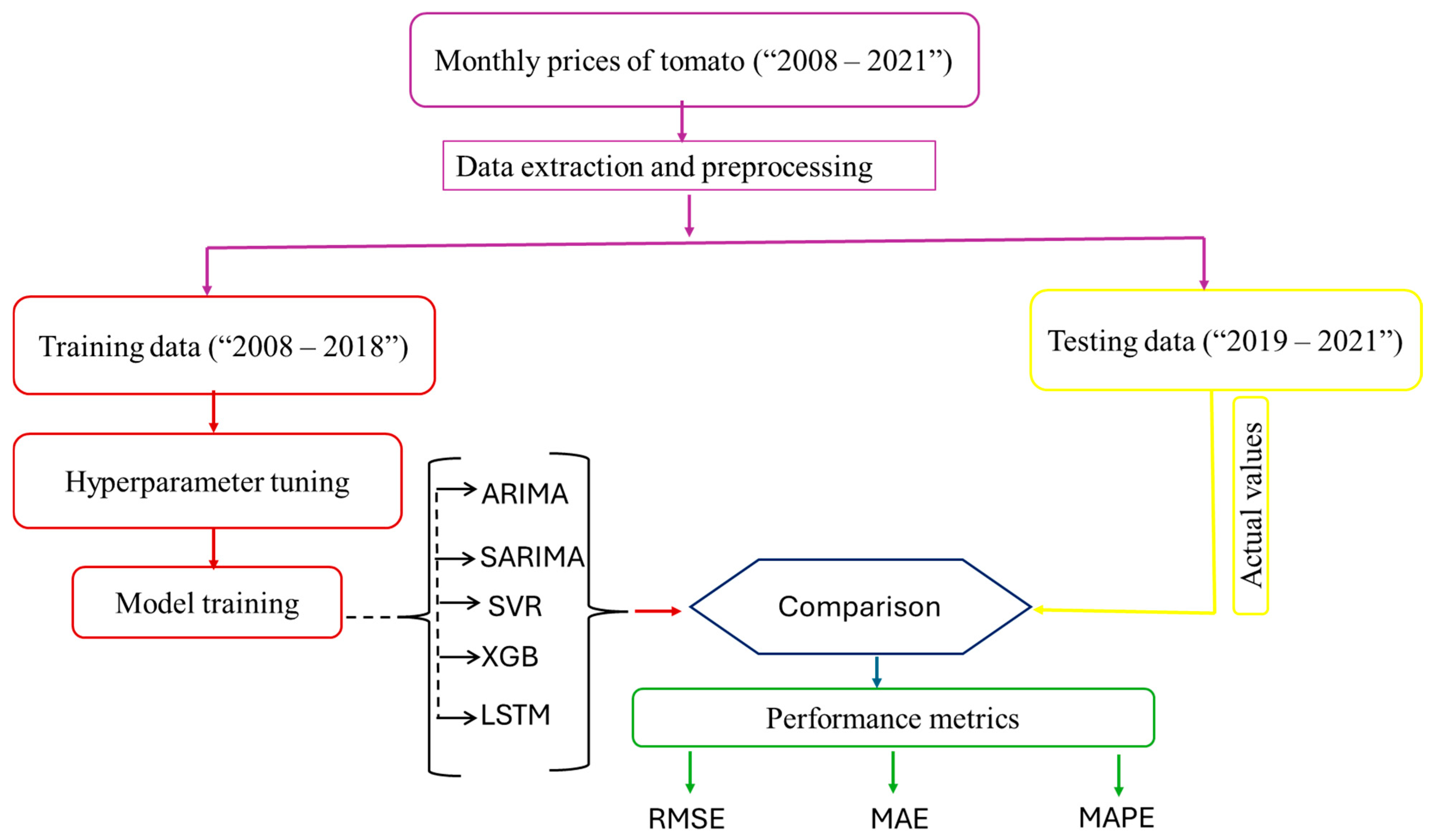
The forecasting ability of different models is assessed with respect to three common performance measures, viz., the root mean squared error (RMSE), the mean absolute error (MAE), and the mean absolute percentage error (MAPE) [24,29]. The equations for estimating these errors are all as given in [24]. Lower values of errors are considered suitable for model evaluation. Figure 1 gives the flowchart of the model development process for tomato price analysis.
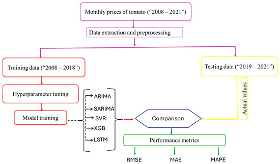
Figure 1.
Flowchart of the model development process.
All analyses were implemented using MATLAB software, version 2024B, on a WINDOWS 10 EliteBook hp personal computer.
3. Results and Discussion
3.1. Data Description
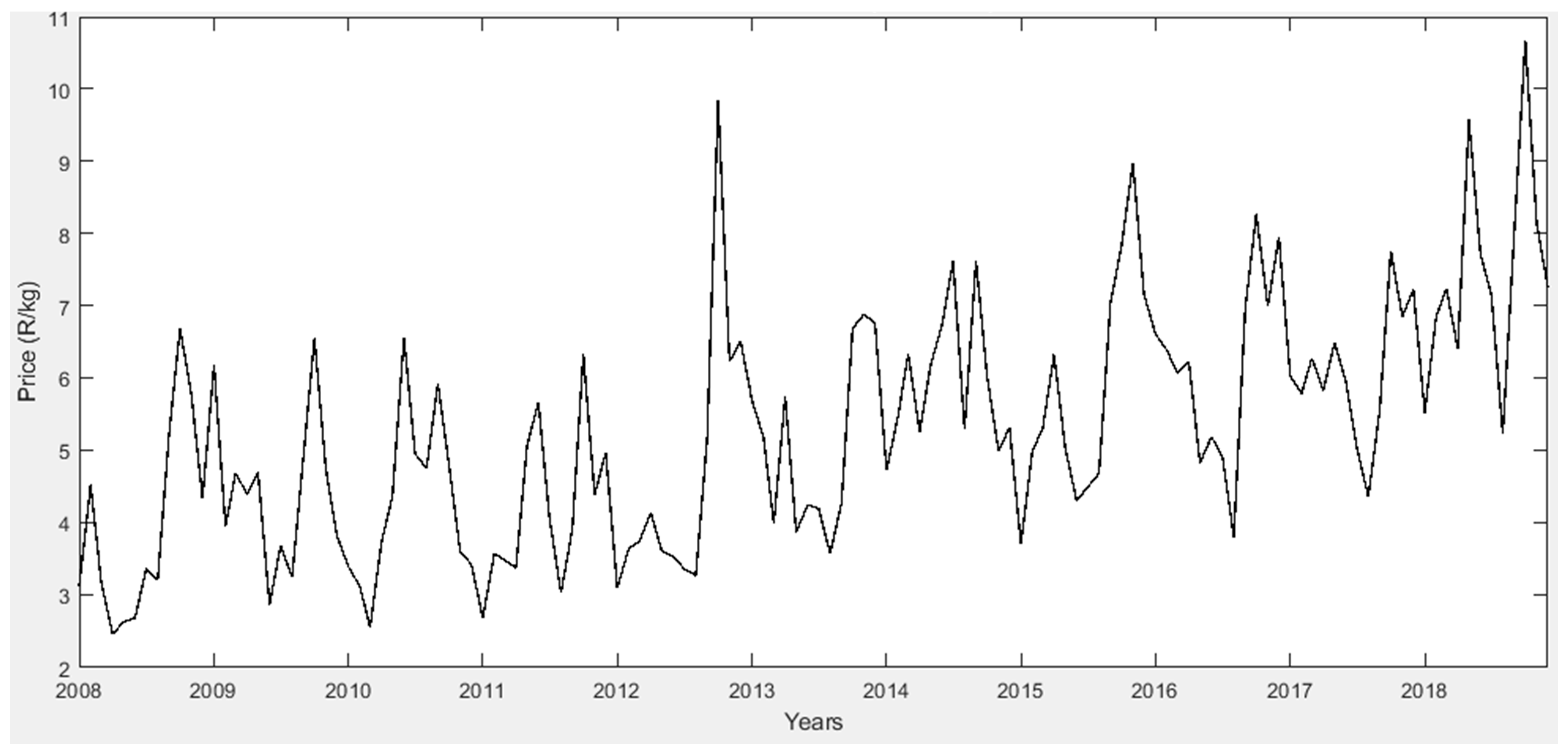
The overall summary of the mean, minimum (Min), maximum (Max), standard deviation (StdDev), skewness, kurtosis, first quartile, second quartile, and third quartile statistics of the monthly price data of tomato are reported in Table 2. An overview of the table shows the average price of tomato. Typically, in time series analysis, data are plotted against monthly prices. Figure 2 shows the time series plot of the average monthly price of tomato from January 2008 to December 2018. An overview of Figure 2 reveals a positive trend over time, which indicates the non-stationary nature of the series. A total of 132 observations (n) were recorded and used to train the models. A seasonal pattern can also be observed. The prices show periodic fluctuations with peaks and troughs, indicating a seasonal trend in tomato prices. A further indication of an overall increasing trend with occasional significant price spikes was noticed, which highlights a potential market or environmental disruption over the period under study.
Table 2.
Summary of monthly tomato price dataset description (n = 132).
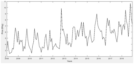
Figure 2.
Monthly price data of tomato from January 2018 to December 2022 (ZAR/kg).
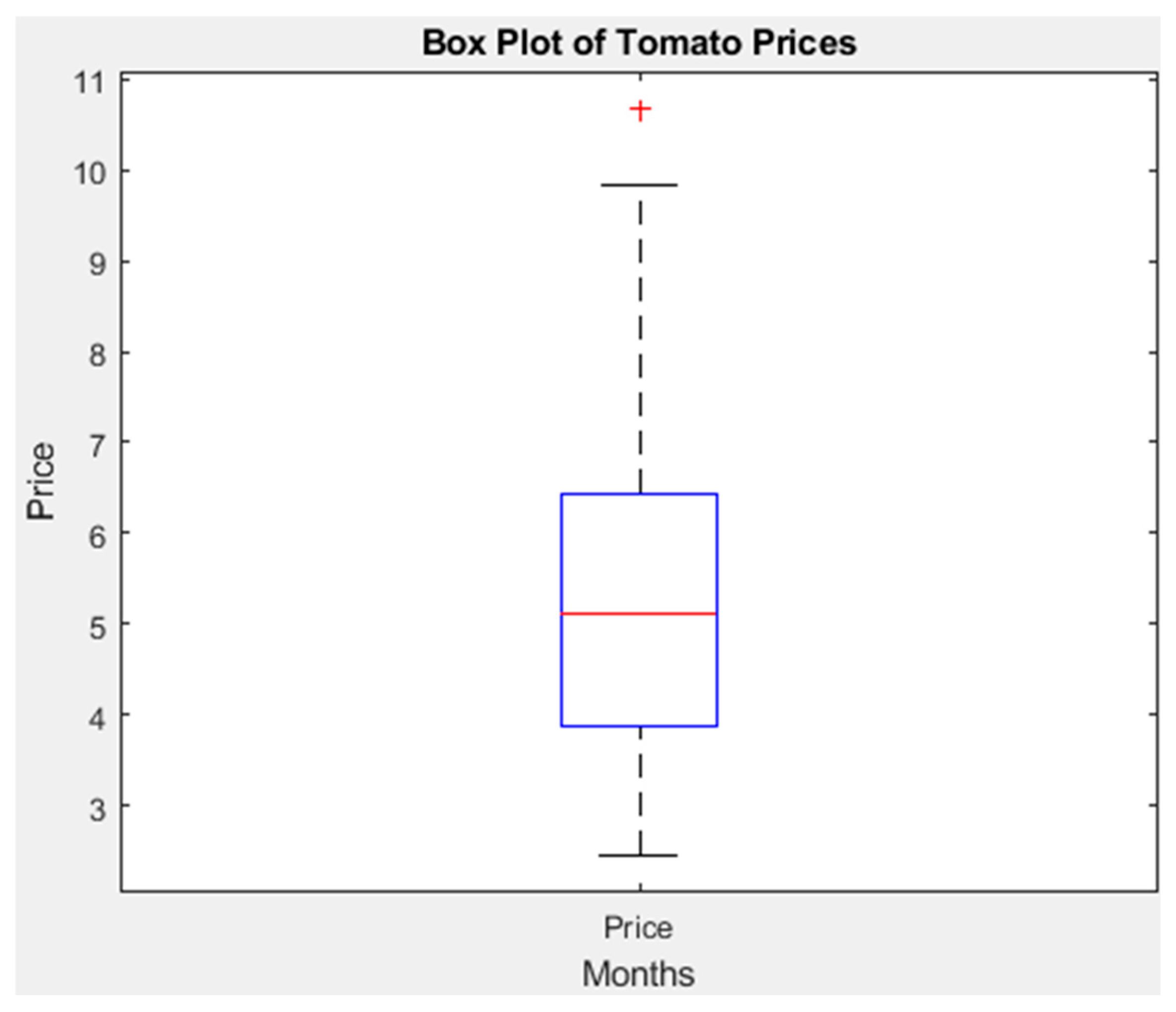
Table 2 shows that the mean price was 5.2861 ZAR/kg and the second quartile (median) was 5.1040 ZAR/kg, and these values closely follow each other. This indicates that the prices slightly deviate from non-normality. Figure 3 shows a box plot of the dataset to further describe the data. In Figure 3, the data display an asymmetric but stable variation during the years considered. An outlier price (red plus symbol) is observed at the top of the box plot. This can likely indicate seasonal price spikes, market fluctuation, and other extreme factors affecting tomato prices.
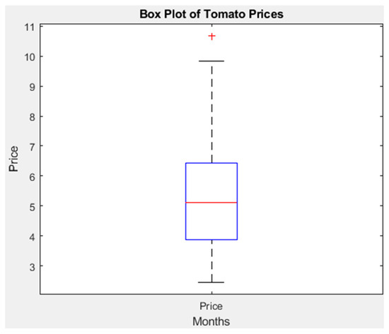
Figure 3.
Box plot showing tomato price distribution from 2008 to 2018; price data from the Cape Town fresh produce market.
Furthermore, the box plot is right-skewed (slightly longer towards the top), which suggests that some months had significantly higher tomato prices compared to others. However, the kurtosis is just slightly above 3, which indicates that data are within a stable variation.
3.2. Data Preprocessing
3.2.1. Non-Stationarity Test
To test for stationarity, the dataset was subjected to the Augmented Dickey–Fuller (ADF) test [36] in order to accurately determine whether to subject the training dataset to differencing before applying ARIMA or SARIMA modeling. Table 3 shows the results of the ADF test. The results indicate that the p-value (0.9298) is much greater than 0.05, which means we fail to reject the null hypothesis. Also, the critical value is higher than the test value, which suggests that our tomato price series data are non-stationary.
Table 3.
Result summary of ADF test (stationarity test) before model development.
After differencing, the tomato price series achieved stationarity and both the ARIMA and SARIMA model were assigned a differential d = 1 in ARIMA (p, 1, q) and SARIMA (p, 1, q) accordingly [36].
3.2.2. Autocorrelation Function (ACF) and Partial Autocorrelation Function (PACF) Analysis
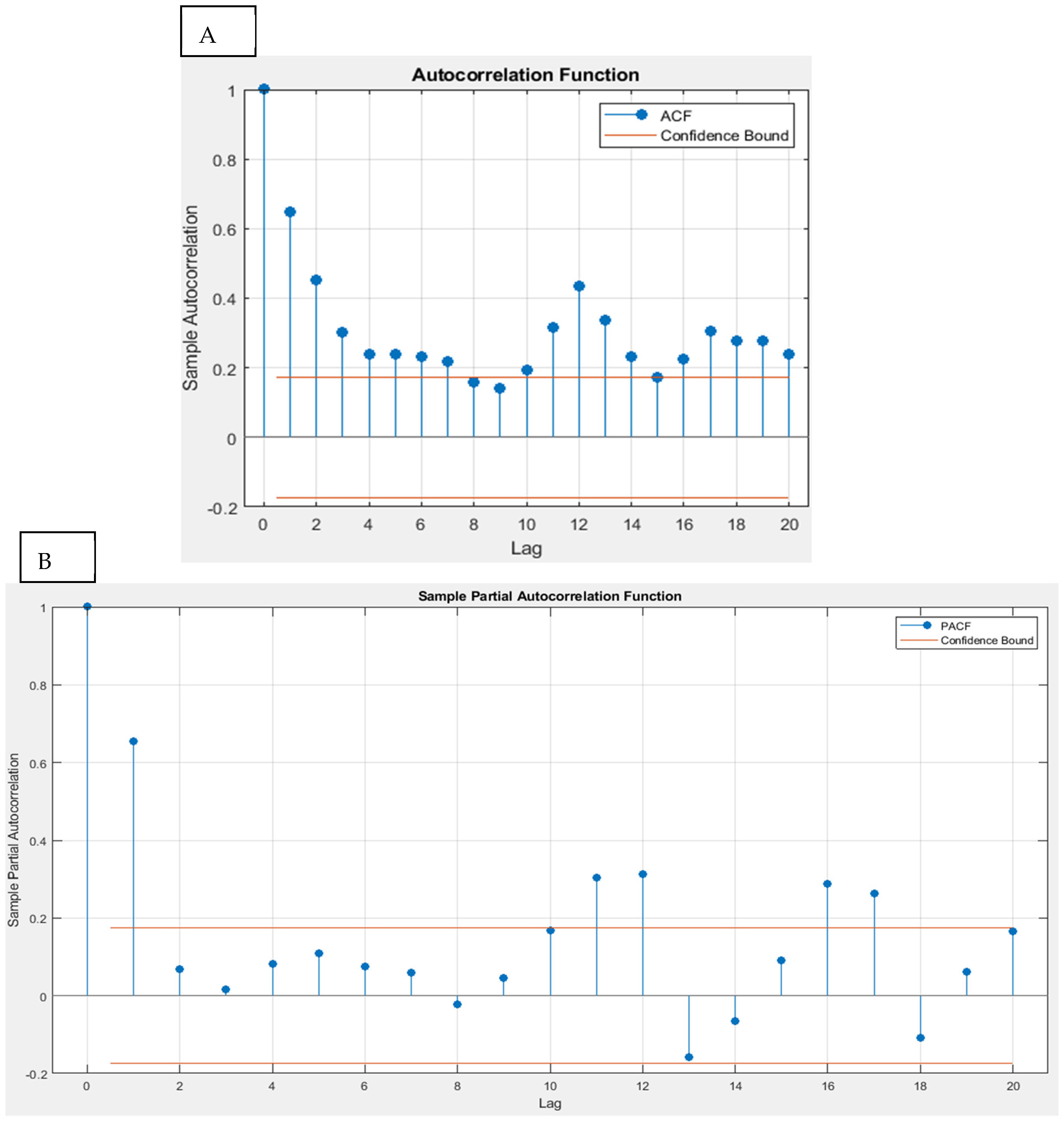
After the stationarity test, autocorrelation function (ACF) and partial autocorrelation function (PACF) analyses were carried out to optimize the performance of the ARIMA and SARIMA model, respectively. The ACF and PACF enhance the performance of ARIMA and SARIMA by indicating the most accurate order of the moving average (MA) and the autoregressive component (AR) of the ARIMA model.
The plots of the ACF and PACF are provided in Figure 4A and Figure 4B, respectively. Figure 4A shows that the first two lags (lag 1 and lag 2) have a highly significant autocorrelation. This can indicate that the data exhibit a strong dependence on past values and may require an MA (q) process (moving average) to be implemented. Furthermore, ACF values are observed to drop gradually after the first two lags, which hints at the non-stationarity of the raw price series data. Some lags beyond lag 10 still have significant autocorrelation, which could indicate seasonality. A similar pattern is observed in Figure 4B. A noticeable spike in lag 1 and lag 2 in the PACF plot is indicative that an AR (p) (2) is required. Hence, the optimal ARIMA model (2, 1, 2) is modeled for the tomato price analysis.
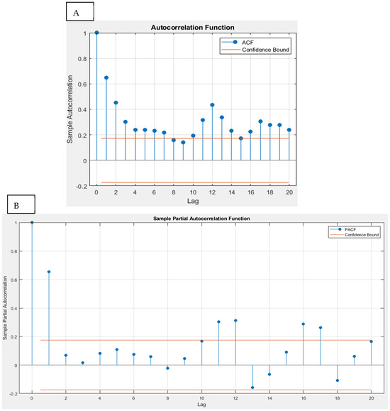
Figure 4.
Plot of autocorrelation function (ACF) (A) and partial autocorrelation function (PACF) (B) for tomato price series.
3.2.3. Nonlinearity Test
Nonlinearity tests allow for an accurate choice of the modeling and prediction of time series data, and it is important to find whether a given time series is nonlinear or not [22]. In this study, Ramsey’s Regression Specification Error Test (RESET) was implemented to provide evidence of nonlinearity or the lack of it. RESET was implemented on the Google Collab platform using python codes. The results are as follows: F-statistic: 2.5400, p-value: 0.1134. Since p > 0.05, this suggests that our tomato time series may be linear.
3.3. Results
Table 4 presents the RMSE, MAE, and MAPE of the different models. In Table 4, lower values for all the performance metrics are indicative of superior performance. The LSTM model stands out as it achieves the lowest RMSE, MAE, and MAPE values.
Table 4.
Summary of results of model performance.
3.3.1. ARIMA Model Result
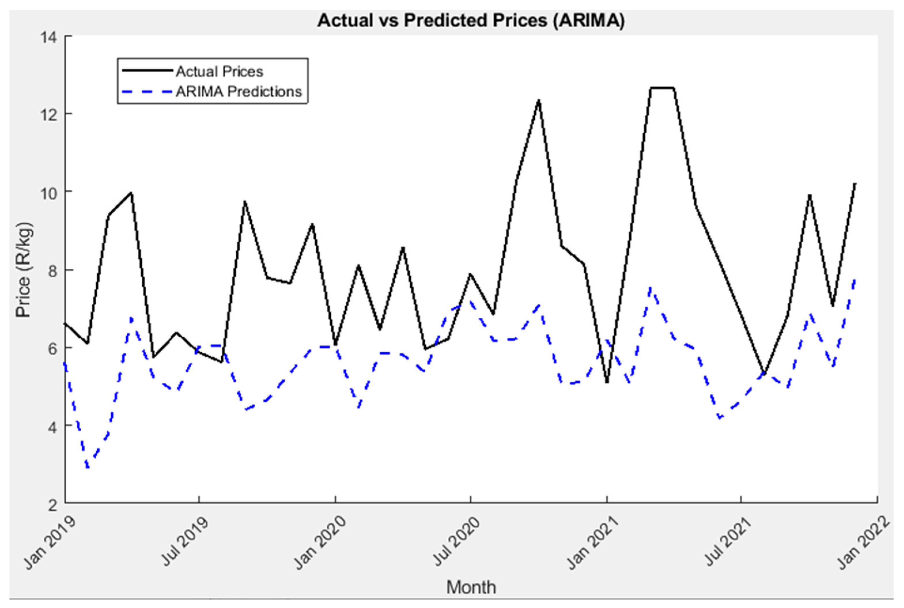
From the results, the ARIMA model showed poor performance, with the highest RMSE (3.0576), MAE (2.5127), and MAPE (28.63%) among the models. Figure 5 shows the performance plot for the ARIMA model.
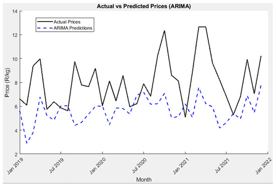
Figure 5.
ARIMA model plot of actual tomato prices against predicted tomato prices for the test dataset (“2019–2021”).
3.3.2. SARIMA Model Result
As shown in Table 4, the SARIMA model results performed relatively well compared to the other models. The model achieved RSME (0.9738), MAE (0.6564), and MAPE (7.66%). It is the second best-performing model in this study. In Figure 6, a plot of actual tomato prices against the predicted prices is presented.
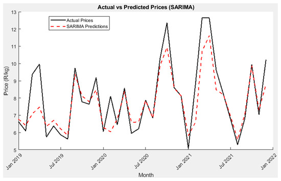
Figure 6.
SARIMA model plot of actual tomato prices against predicted tomato prices for the test dataset (“2019–2021”).
3.3.3. SVR Model Result
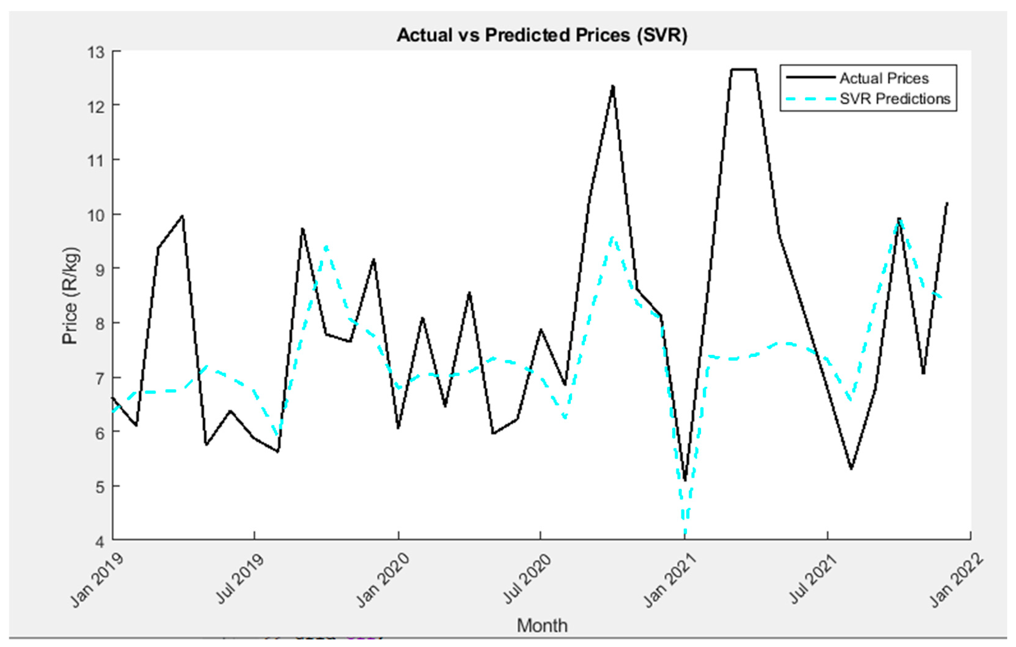
The SVR model only outperformed the ARIMA model, with results showing RMSE (1.8535), MAE (1.4089), and MAPE (16.44%), the highest values among the models. Figure 7 shows the plot of the actual vs. predicted values for the SVR model.
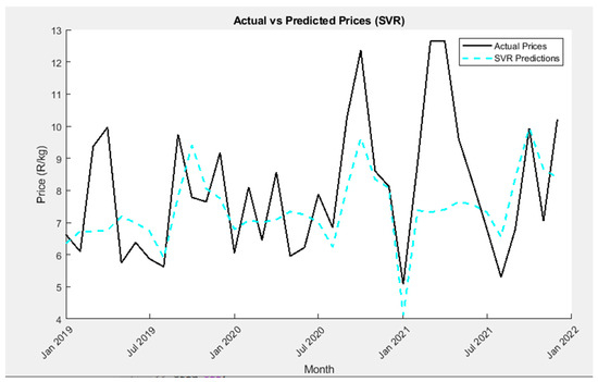
Figure 7.
SVR model plot of actual tomato prices against predicted tomato prices for the test dataset (“2019–2021”).
3.3.4. XGB Model Result
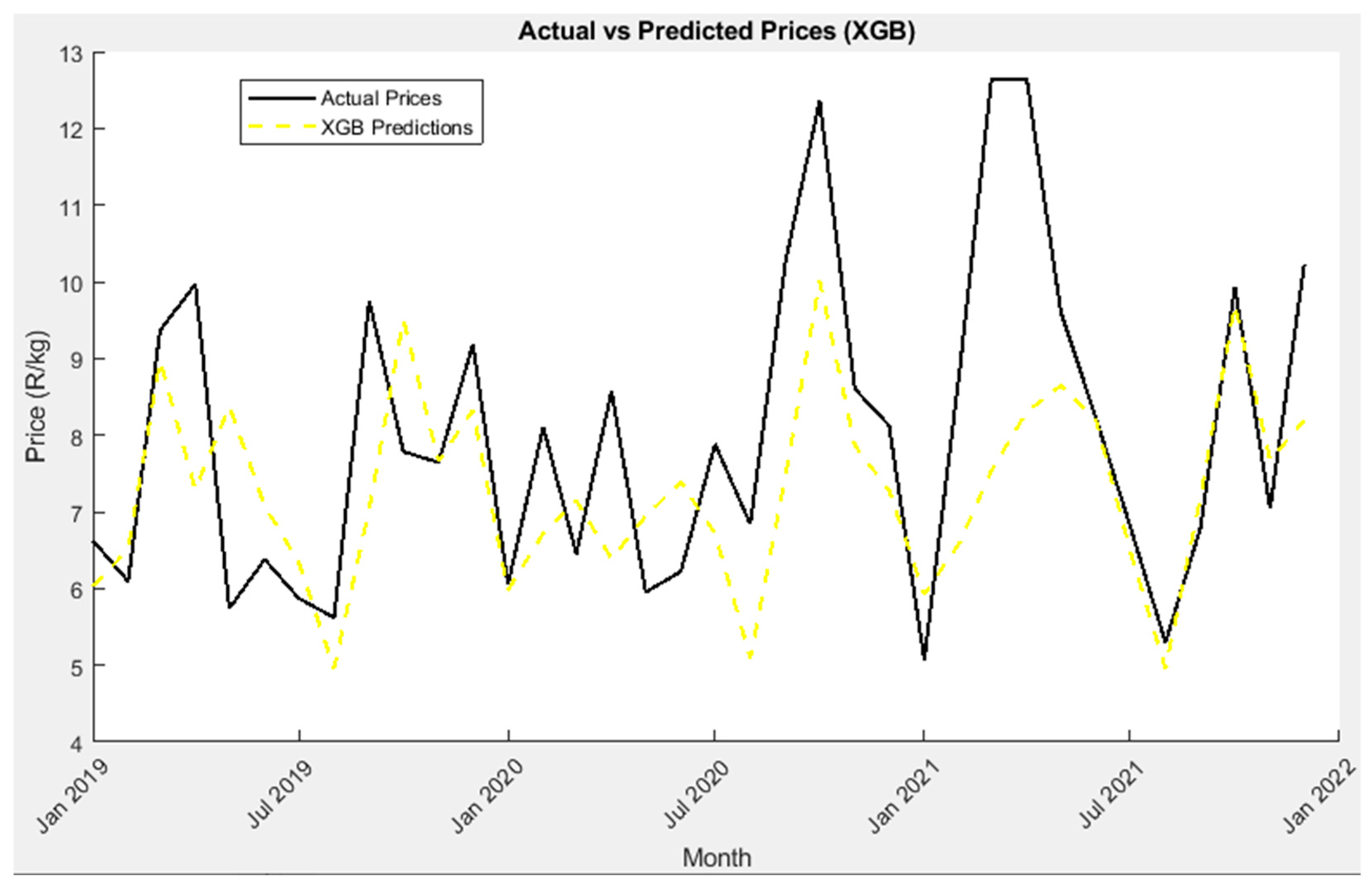
The XGB model outperformed the SVR model in terms of future tomato price forecasting. The model performance in Table 4 shows that XGB obtained an RMSE (1.7637), MAE (1.3184), and MAPE (15.38%). It is the best-performing traditional ML model among the two compared. Figure 8 shows the plot of the actual vs. predicted values for the XGB model.
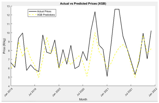
Figure 8.
XGB model plot of actual tomato prices against predicted tomato prices for the test dataset (“2019–2021”).
3.3.5. LSTM Model Result
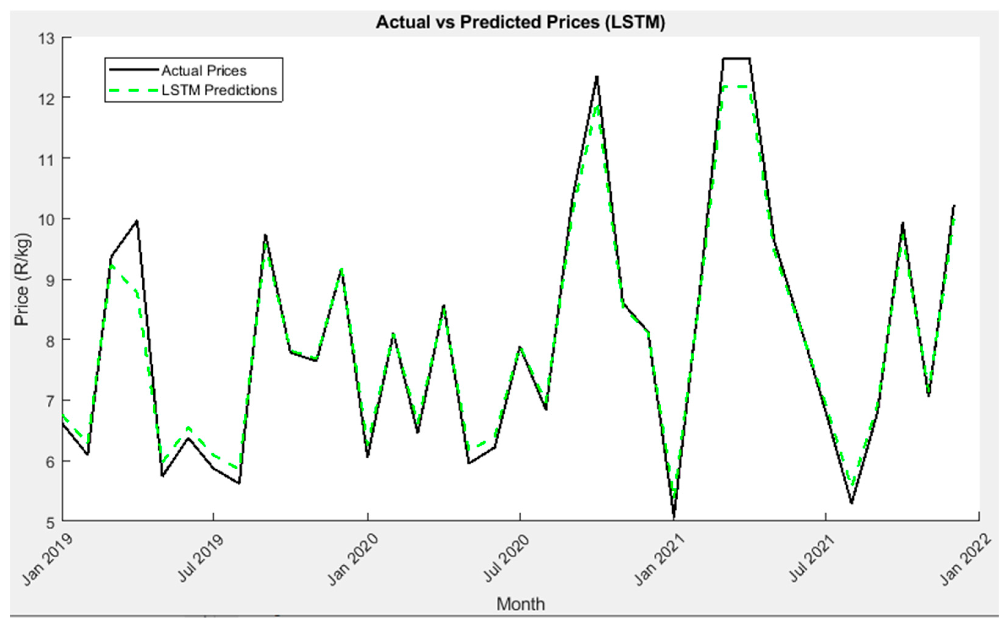
The LSTM proved to be the best-performing model in terms of price forecasting of tomato prices. It obtained the lowest RMSE (0.2818), MAE (0.1925), and MAPE (2.42%). The model performance, showing the predicted prices against the actual price values, is presented in Figure 9. From Figure 9, it can be observed that the predicted prices closely follow the actual price values.
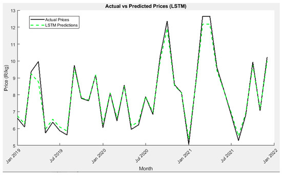
Figure 9.
LSTM model plot of actual tomato prices against predicted tomato prices for the test dataset (“2019–2021”).
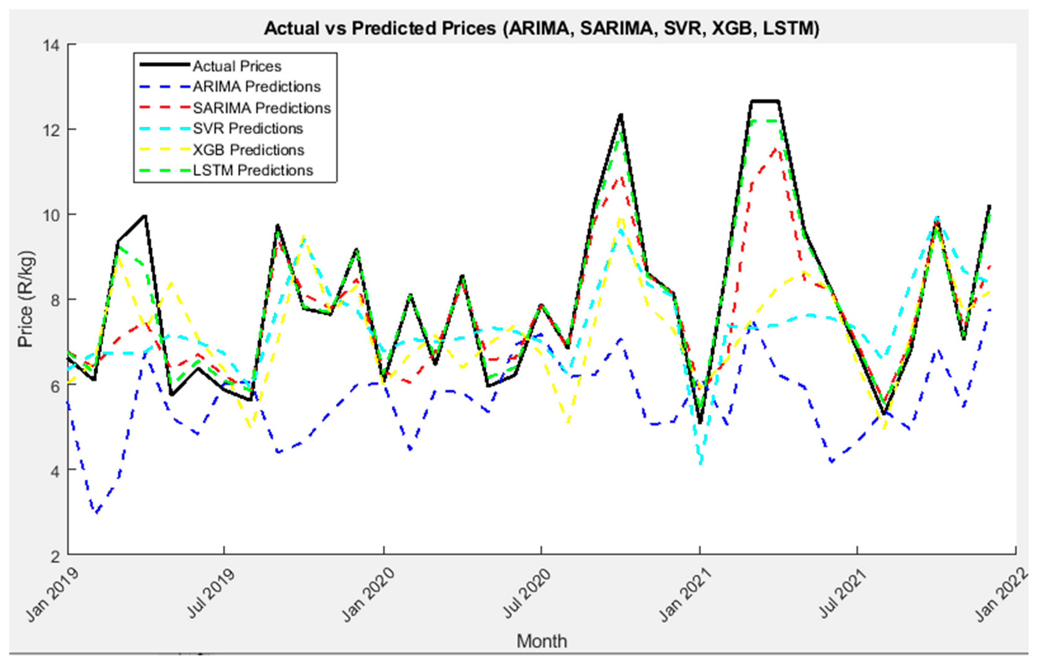
The combined model is provided in Figure 10. In Figure 10, we notice that the SARIMA model (red dotted lines) and the LSTM model (green dotted lines) closely follow the price trend of the actual or real price values, which further elucidates the accuracy and reliability of the models.

Figure 10.
The combined plot of actual vs. predicted prices for all the models used for tomato price forecasting analysis (“2019–2021”).
3.4. Discussion
This study has comparatively considered the model performance of several price forecasting approaches for the price prediction of future tomato prices. Two standard econometric models (ARIMA and SARIMA) as well as two popular traditional machine learning approaches (SVR and XGB) have been compared to the deep learning-based LSTM model. This study further includes comprehensive analyses such as data preprocessing, autocorrelation (ACF) and partial autocorrelation (PACF) evaluations, and tests for non-stationarity and nonlinearity to enhance the robustness and validity of the results.
The findings show that the LSTM approach is superior to the conventional approaches considered. Similar studies have reported that the LSTM outperforms conventional ML-based approaches for various types of agricultural produce. For instance, Nassar et al. [23] compared LSTM with ARIMA and XGB. They found that LSTM achieved an RMSE of 1.22 compared to 1.28 for XGB in price prediction for cabbage, cauliflower, bok choi, and watermelon. However, a hybrid-based CNN-LSTM with an additional attention mechanism was used to further improve the model performance by a further 19% and 10%, respectively. In another comparative study with five (5) major predictions, Paul et al. [37] compared price prediction for brinjal (eggplant) using price data. The deep learning-based G-RNN yielded better model performance for the commodity from different localities based on ME, RMSE, MAE, and MAPE values. However, the author applied daily wholesale price data for their analysis.
The LSTM model’s performance nearly mirrors the performance of LSTM for the price forecasting analysis of celery [3]. The authors reported RMSE (0.226), MAE (0.131), and R2 (0.953). In the current study, an R2 value of 0.9807 was attained. Although daily price data were used for the study, the LSTM model performed similarly, thereby proving LSTM’s generalization capability. Like the findings of this study, Patil et al. [27] found that SARIMA and LSTM outperformed other methods in terms of future price prediction analysis for five important commodities (wheat, millet, sorghum, maize, and rice). However, the authors only reported the MAPE values in their study.
Typically, seasonality causes data series to be nonstationary, which is expected for tomato price data [38]; this explains why the SARIMA model showed good forecasting capabilities. This was highlighted as LSTM’s capabilities to handle linearity and other intricate time series features were explored for better model performance [22]. However, the authors report that improved performance can be further achieved with model hybridization.
Although this study exclusively utilized data from the Cape Town fresh produce market (FPM), tomatoes exhibit comparable seasonality patterns and market dynamics across other regions in South Africa. Therefore, the forecasting approach presented here is broadly applicable and could be adopted for other FPMs nationwide. To further enhance the generalizability and accuracy of the findings, future research could investigate various hybrid deep learning models to optimize forecasting performance for tomato price analysis.
4. Conclusions
This study investigated models for the prediction and forecasting of tomato prices from the Cape Town fresh produce market using monthly price data from 2008 to 2021 by means of a deep learning-based LSTM method. A comparative analysis was performed against four other well-known forecasting models. The results show that LSTM outperformed all other approaches for prediction and forecasting applications. The SARIMA model closely followed the LSTM model in terms of its performance; however, ARIMA showed very poor performance and should not be encouraged for tomato price modeling applications.
Although this study focused on tomato prices, the developed model could be adapted for other agricultural commodities. The forecast of future prices reveals that the prices of tomatoes will be stable over the next 10 years. These forecasted prices present a valuable insight and serve as a critical decision making tool for stakeholders in the agribusiness sector, supporting sustainable tomato production, food security, and profitability within the fresh produce supply chain. Future studies could further enhance forecasting accuracy by integrating additional agricultural variables that directly influence tomato pricing and production. Furthermore, optimized forecasting models have the potential to be incorporated into real-time decision support systems, thereby significantly improving the effectiveness of the fresh produce supply chain.
Author Contributions
Conceptualization, methodology, software, validation, formal analysis, investigation, resources, data curation, writing—original draft preparation, E.E.O.; writing—review and editing, visualization, supervision, project administration, funding acquisition, V.B. All authors have read and agreed to the published version of the manuscript.
Funding
This research received no external funding.
Data Availability Statement
All data sources used for this study are available and accessible on published sources and can be made available on request.
Acknowledgments
We acknowledge the National Agricultural Marketing Council (NAMC), the Department of Agriculture, Forestry and Fisheries (DAFF), Statistics South Africa (SSA), and the Department of Agriculture, Land Reform and Rural Development (DALRRD) for their annual reports and data resources, which contributed greatly to this research.
Conflicts of Interest
The authors declare no conflicts of interest.
References
- Sun, F.; Meng, X.; Zhang, Y.; Wang, Y.; Jiang, H.; Liu, P. Agricultural product price forecasting methods: A review. Agriculture 2023, 13, 1671. [Google Scholar] [CrossRef]
- Wihartiko, F.D.; Nurdiati, S.; Buono, A.; Santosa, E. Agricultural price prediction models: A systematic literature review. In Proceedings of the International Conference on Industrial Engineering and Operations Management, Singapore, 7–11 March 2021; IEOM Society International: Southfield, MI, USA, 2021; pp. 2927–2934. [Google Scholar] [CrossRef]
- Zhang, Q.; Yang, W.; Zhao, A.; Wang, X.; Wang, Z.; Zhang, L. Short-term forecasting of vegetable prices based on LSTM model—Evidence from Beijing’s vegetable data. PLoS ONE 2024, 19, e0304881. [Google Scholar] [CrossRef] [PubMed]
- Santoso, I.; Purnomo, M.; Sulianto, A.A.; Choirun, A. Machine learning application for sustainable agri-food supply chain performance: A review. In Proceedings of the IOP Conference Series: Earth and Environmental Science, Banda Aceh, Indonesia, 21 September 2021; IOP Publishing Ltd.: Bristol, UK, 2021. [Google Scholar] [CrossRef]
- Zhao, C.; Wang, X.; Zhao, A.; Cui, Y.; Wang, T.; Liu, J.; Hou, Y.; Wang, M.; Chen, L.; Li, H.; et al. A vegetable-price forecasting method based on mixture of experts. Agriculture 2025, 15, 162. [Google Scholar] [CrossRef]
- Opara, I.K.; Fawole, O.A.; Opara, U.L. Postharvest losses of pomegranate fruit at the packhouse and implications for sustainability indicators. Sustainability 2021, 9, 5187. [Google Scholar] [CrossRef]
- Opara, I.K.; Fawole, O.A.; Kelly, C.; Opara, U.L. Quantification of on-farm pomegranate fruit postharvest losses and waste, and implications on sustainability indicators: South African case study. Sustainability 2021, 13, 5168. [Google Scholar] [CrossRef]
- Beckert, J. Where Do Prices Come from? Sociological Approaches to Price Formation; Max Planck Institute for the Study of Societies: Cologne, Germany, 2011; Available online: https://hdl.handle.net/10419/45619 (accessed on 14 February 2025).
- Yin, H.; Jin, D.; Gu, Y.H.; Park, C.J.; Han, S.K.; Yoo, S.J. STL-ATTLSTM: Vegetable price forecasting using stl and attention mechanism-based LSTM. Agriculture 2020, 10, 612. [Google Scholar] [CrossRef]
- Baiyegunhi, L.; Sharaunga, S.; Dlangisa, S.; Ndaba, N. Tomato market integration: A case study of the Durban and Johannesburg fresh produce markets in South Africa. J. Agribus. Rural Dev. 2018, 49, 239–249. [Google Scholar] [CrossRef]
- Directorate: Statistics and Economic Analysis. Abstract of Agricultural Statistics. Department of Agriculture, Land Reform & Rural Development, 2024. Pretoria, Republic of South Africa. Available online: https://www.dalrrd.gov.za/images/Branches/Economica%20Development%20Trade%20and%20Marketing/Statistc%20and%20%20Economic%20Analysis/statistical-information/abstract-2024.pdf (accessed on 14 February 2025).
- Department of Agriculture, Land Reform and Rural Development, Resource Centre. 2025. Available online: https://old.dalrrd.gov.za/Resource-Centre?folderId=377&view=gridview&pageSize=2147483647 (accessed on 14 February 2025).
- National Agricultural Marketing Council (NAMC). The-SA-Tomato-Value-Chain-Desktop-Study-2023-24. 2024. Available online: https://www.namc.co.za/wp-content/uploads/2024/03/The-SA-Tomato-Value-Chain-Desktop-Study-2023-24.pdf (accessed on 14 February 2025).
- Cherono, K. Development and Optimization of an Integrated Postharvest Management System for Storage and Handling of Fresh Market Tomatoes in South African Supply Chains. Ph.D. Thesis, University of KwaZulu-Natal, Pietermaritzburg, South Africa, 2016. [Google Scholar]
- Korsten, L. Postharvest Losses of Fresh Produce. The African Academy of Sciences, 2024. University of Pretoria. Available online: https://stopmedwaste.net/wp-content/uploads/2024/01/Postharvest-losses-of-Fresh-produce.pdf (accessed on 14 February 2025).
- Choong, K.Y.; Raof, R.A.A.; Sudin, S.; Ong, R.J. Time series analysis for vegetable price forecasting in e-commerce platform: A review. J. Phys. Conf. Ser. 2021, 1878, 012071. [Google Scholar] [CrossRef]
- Mienye, I.D.; Swart, T.G. A Comprehensive Review of deep learning: Architectures, recent advances, and applications. Information 2024, 15, 755. [Google Scholar] [CrossRef]
- Jin, B.; Xu, X. Predicting wholesale edible oil prices through Gaussian process regressions tuned with Bayesian optimization and cross-validation. Asian J. Econ. Bank. 2025, 9, 64–82. [Google Scholar] [CrossRef]
- Lim, B.; Zohren, S. Time-series forecasting with deep learning: A survey. Philos. Trans. R. Soc. A 2021, 379, 20200209. [Google Scholar] [CrossRef] [PubMed]
- Yuan, C.Z.; Ling, S.K. Long short-term memory model based agriculture commodity price prediction application. In Proceedings of the 2020 2nd International Conference on Information Technology and Computer Communications, Kuala Lumpur, Malaysia, 12–14 August 2020; pp. 43–49. [Google Scholar] [CrossRef]
- Murugesan, R.; Mishra, E.; Krishnan, A.H. Deep Learning Based Models: Basic LSTM, Bi LSTM, Stacked LSTM, CNN LSTM and Conv LSTM to forecast agricultural commodities prices. Res. Sq. 2021, 1, 1–32. [Google Scholar] [CrossRef]
- Avinash, G.; Ramasubramanian, V.; Paul, R.K.; Ray, M.; Dahiya, S.; Iquebal, M.A.; Godara, S.; Manjunatha, B. Price forecasting of top (tomato, onion and potato) commodities using Hidden Markov-based Deep learning approach. Stat. Appl. 2024, 22, 63–90. Available online: http://www.ssca.org.in/journal (accessed on 14 February 2025).
- Nassar, L.; Okwuchi, I.E.; Saad, M.; Karray, F.; Ponnambalam, K. Deep learning based approach for fresh produce market price prediction. In Proceedings of the International Joint Conference on Neural Networks (IJCNN), Glasgow, UK, 19–24 July 2020. [Google Scholar]
- Okwuchi, I.E. Machine Learning Based Models for Fresh Produce Yield and Price Forecasting for Strawberry Fruit. Master’s Thesis, University of Waterloo, Waterloo, ON, Canada, 2020. Available online: http://hdl.handle.net/10012/15976 (accessed on 14 February 2025).
- Kumari, P.; Goswami, V.; Harshith, N.; Pundir, R.S. Recurrent neural network architecture for forecasting banana prices in Gujarat, India. PLoS ONE 2023, 18, e0275702. [Google Scholar] [CrossRef]
- Srichaiyan, P.; Tippayawong, K.Y.; Boonprasope, A. Forecasting soybean futures prices with adaptive AI Models. IEEE Access 2025, 13, 48239–48256. [Google Scholar] [CrossRef]
- Patil, A.; Shah, D.; Shah, A.; Kotecha, R. Forecasting prices of agricultural commodities using machine learning for global food security: Towards sustainable development goal 2. Int. J. Eng. Trends Technol. 2023, 71, 277–291. [Google Scholar] [CrossRef]
- Jha, G.K.; Sinha, K. Agricultural price forecasting using neural network model: An innovative information delivery system. Agric. Econ. Res. Rev. 2013, 26, 229–239. [Google Scholar] [CrossRef]
- Nassar, L.; Okwuchi, I.E.; Saad, M.; Karray, F.; Ponnambalam, K.; Agrawal, P. Prediction of strawberry yield and farm price utilizing deep learning. In Proceedings of the International Joint Conference on Neural Networks (IJCNN), Glasgow, UK, 19–24 July 2020. [Google Scholar] [CrossRef]
- Haofei, Z.; Guoping, X.; Fangting, Y.; Han, Y. A neural network model based on the multi-stage optimization approach for short-term food price forecasting in China. Expert Syst. Appl. 2007, 33, 347–356. [Google Scholar] [CrossRef]
- Box, G.E.P.; Jenkins, G.M.; Reinsel, G.C. Time Series Analysis-Forecasting and Control, 3rd ed.; Prentice-Hall Inc.: Upper Saddle River, NJ, USA, 1994; ISBN 0-13-060774-6. [Google Scholar]
- Vapnik, V. The Nature of Statistical Learning Theory, 2nd ed.; Springer: Berlin/Heidelberg, Germany, 1995; ISBN 0-387-98780-0. [Google Scholar]
- Wang, Y.; Zhu, S.; Li, C. Research on multistep time series prediction based on LSTM. In Proceedings of the 2019 3rd International Conference on Electronic Information Technology and Computer Engineering (EITCE), Xiamen, China, 18–20 October 2019; IEEE Xplore: Piscataway, NJ, USA, 2019; pp. 1155–1159. [Google Scholar] [CrossRef]
- Gers, F.A.; Schmidhuber, J.; Cummins, F. Learning to Forget: Continual Prediction with LSTM. Neural Comput. 2000, 12, 2451–2471. [Google Scholar] [CrossRef]
- Gers, F.A.; Schraudolph, N.N.; Schmidhuber, J. Learning precise timing with LSTM recurrent networks. J. Mach. Learn. Res. 2002, 3, 115–143. Available online: https://www.jmlr.org/papers/v3/gers02a.html (accessed on 14 February 2025).
- Menculini, L.; Marini, A.; Proietti, M.; Garinei, A.; Bozza, A.; Moretti, C.; Marconi, M. Comparing prophet and deep learning to ARIMA in forecasting wholesale food prices. Forecasting 2021, 3, 644–662. [Google Scholar] [CrossRef]
- Paul, R.K.; Yeasin, M.; Kumar, P.; Kumar, P.; Balasubramanian, M.; Roy, H.S.; Paul, A.K.; Gupta, A. Machine learning techniques for forecasting agricultural prices: A case of brinjal in Odisha, India. PLoS ONE 2022, 17, e0270553. [Google Scholar] [CrossRef] [PubMed]
- Reddy, A.A. Price forecasting of tomatoes. Int. J. Veg. Sci. 2018, 25, 176–184. [Google Scholar] [CrossRef]

Disclaimer/Publisher’s Note: The statements, opinions and data contained in all publications are solely those of the individual author(s) and contributor(s) and not of MDPI and/or the editor(s). MDPI and/or the editor(s) disclaim responsibility for any injury to people or property resulting from any ideas, methods, instructions or products referred to in the content. |
© 2025 by the authors. Licensee MDPI, Basel, Switzerland. This article is an open access article distributed under the terms and conditions of the Creative Commons Attribution (CC BY) license (https://creativecommons.org/licenses/by/4.0/).