Day-Ahead Energy Price Forecasting with Machine Learning: Role of Endogenous Predictors

Abstract

Accurate Day-Ahead Energy Price (DAEP) forecasting is essential for optimizing energy market operations. This study introduces a machine learning framework to predict the DAEP with a 24 h lead time, leveraging historical data and forecasts available at the prediction time. Hourly DAEP data from the California Independent System Operator (January 2017 to July 2023) were integrated with exogenous and engineered endogenous features. A custom rolling window cross-validation, with 24 h validation blocks sliding daily across 2372 folds, evaluates an Extreme Gradient Boosting (XGBoost) model’s performance under diverse market conditions, achieving a median mean absolute error of 6.26 USD/MWh and root mean squared error of 8.27 USD/MWh, with variability reflecting market volatility. The feature importance analysis using Shapley additive explanations highlighted the dominance of engineered endogenous features in driving the 24 h lead time forecasts under relatively stable market conditions. Forecasting the DAEP at a runtime of 10 AM on the prior day was used to assess model uncertainty. This involved training random forest, support vector regression, XGBoost, and feed forward neural network models, followed by stacking and voting ensembles. The results indicate the need for ensemble forecasting and evaluation beyond a static train–test split to ensure the practical utility of machine learning for DAEP forecasting across varied market dynamics. Finally, operationalizing the forecast model for bidding decisions by forecasting the DAEP and real-time prices at runtime is presented and discussed.

1. Introduction

Accurate forecasting of energy prices is critical for bolstering market intelligence and enabling informed decision-making in the energy sector, where price volatility directly impacts utilities, traders, and grid operators [1,2]. Effective market intelligence enhances energy security, optimizes resource allocation, and supports economic growth by giving stakeholders insights into uncertain pricing dynamics [3]. In recent decades, the growing integration of renewable energy sources, like wind and solar, which are projected to expand further due to technological advancements and supportive policies, has amplified the importance of precise price forecasts [4,5,6,7]. However, renewable energy sources’ intermittent and variable nature, driven by weather-dependent generation patterns, introduces significant challenges to grid stability and market operations [8,9]. This variability can lead to voltage fluctuations, frequency deviations, and supply–demand mismatches, heightening the need for reliable forecasting to manage costs and ensure grid reliability for utilities and market participants [10,11].

In energy market bidding, participants must strategically choose between selling electricity in the Day-Ahead Energy Price (DAEP) market, where prices are set one day in advance based on anticipated supply and demand, and the Real-Time (RT) market, where prices fluctuate hourly based on immediate grid conditions. Grid stability challenges are exacerbated by the need for accurate price forecasting in deregulated energy markets, where the DAEP dictates bidding strategies, risk management, and resource allocation [12,13]. The volatility of renewable energy complicates these forecasts, as sudden shifts in wind speed, solar insolation, or load demand can lead to significant price fluctuations [14,15]. Traditional (linear) forecasting methods often struggle to capture these dynamic market conditions, necessitating advanced techniques to ensure grid stability and market efficiency [16,17].

Machine Learning (ML) has become a transformative tool in addressing the challenges in forecasting energy market conditions, offering predictive capabilities that adapt to non-linear patterns in market data [18,19]. ML models, including Extreme Gradient Boosting (XGBoost) [20], Support Vector Regression (SVR) [21], and Random Forests (RF) [22], among others, excel at integrating diverse predictors—such as weather forecasts, load data, and historical prices—into forecasts, stabilizing grid operations by enabling proactive scheduling and balancing [23].

Several studies have applied ML in forecasting in the energy sector, including the DAEP [24,25,26]. For instance, ref. [27] utilized a bionic optimization algorithm combined with ML to enhance the accuracy of DAEP forecasting. Similarly, ref. [28] applied XGBoost for day-ahead load forecasting. Despite these advancements in ML applications, DAEP forecasting faces notable challenges primarily due to market volatility. A predominant issue in the robust evaluation of forecast models is the reliance on fixed train–test splits, which may fail to capture both short-term and long-term market dynamics. While rolling evaluations have been explored (e.g., [29]), they are not yet widely adopted. Additionally, feature importance analysis to rank predictors and the relative role of a comprehensive set of engineered endogenous variables that capture the daily, weekly, and seasonal cyclic patterns of the DAEP remain underutilized. Therefore, this study aims to develop a scalable framework for forecasting the DAEP at least 24 h ahead by addressing the following tasks: (1) utilizing a comprehensive set of endogenous variables to capture the temporal structure of the DAEP across daily, weekly, and seasonal timeframes and assessing their importance in the forecast model using SHapley Additive exPlanations (SHAP) analysis [30]; (2) evaluating model performance across diverse market conditions through a 24 h rolling window validation approach; and (3) addressing forecast model uncertainty by comparing the performance of XGBoost, SVR, RF, and Feed-Forward Neural Network (FFNN) while investigating the added value of ensemble techniques, such as stacking [31] and averaging [32]. Through these tasks, this research seeks to enhance market intelligence for energy market stakeholders, enabling more informed decision-making in volatile energy markets.

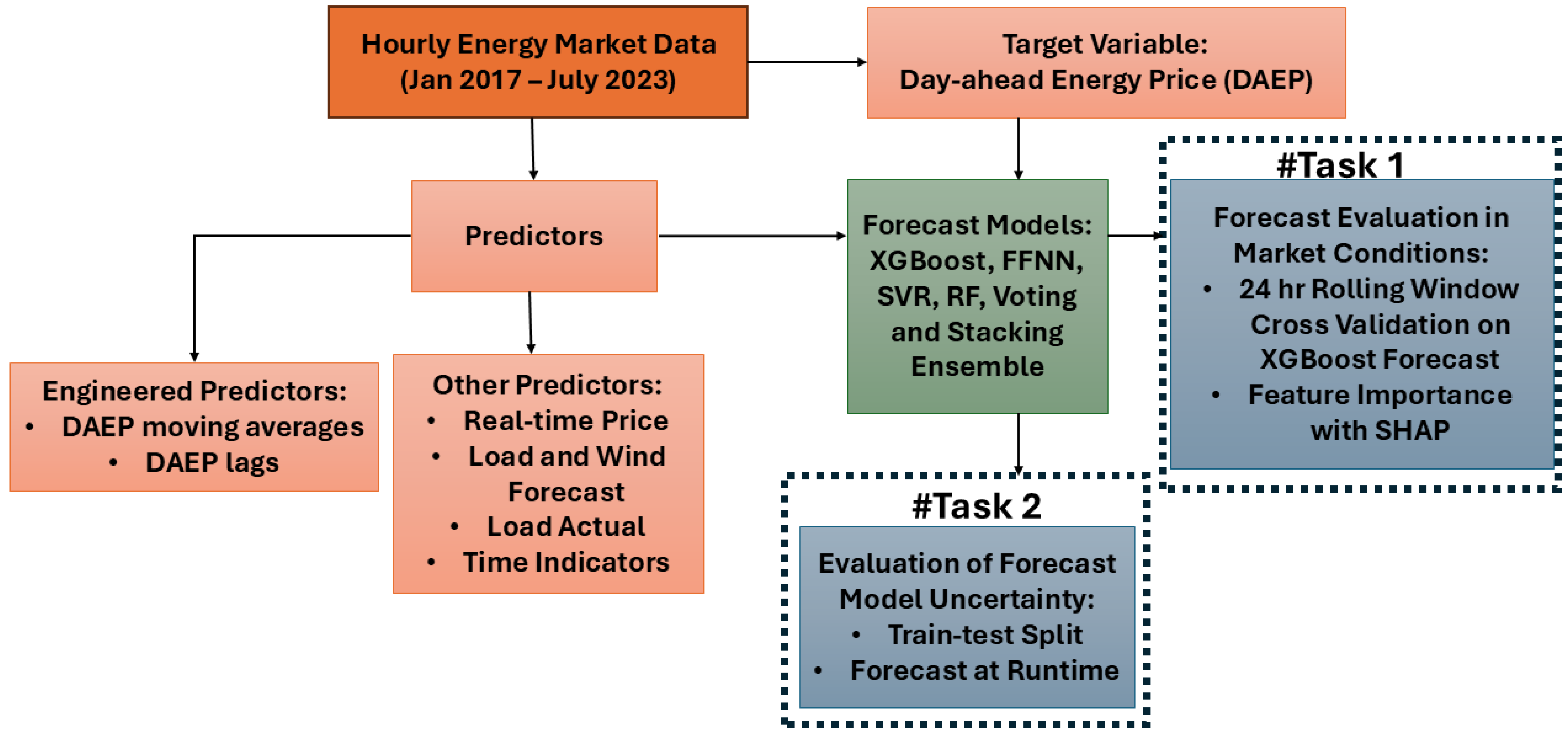
2. Materials and Methods

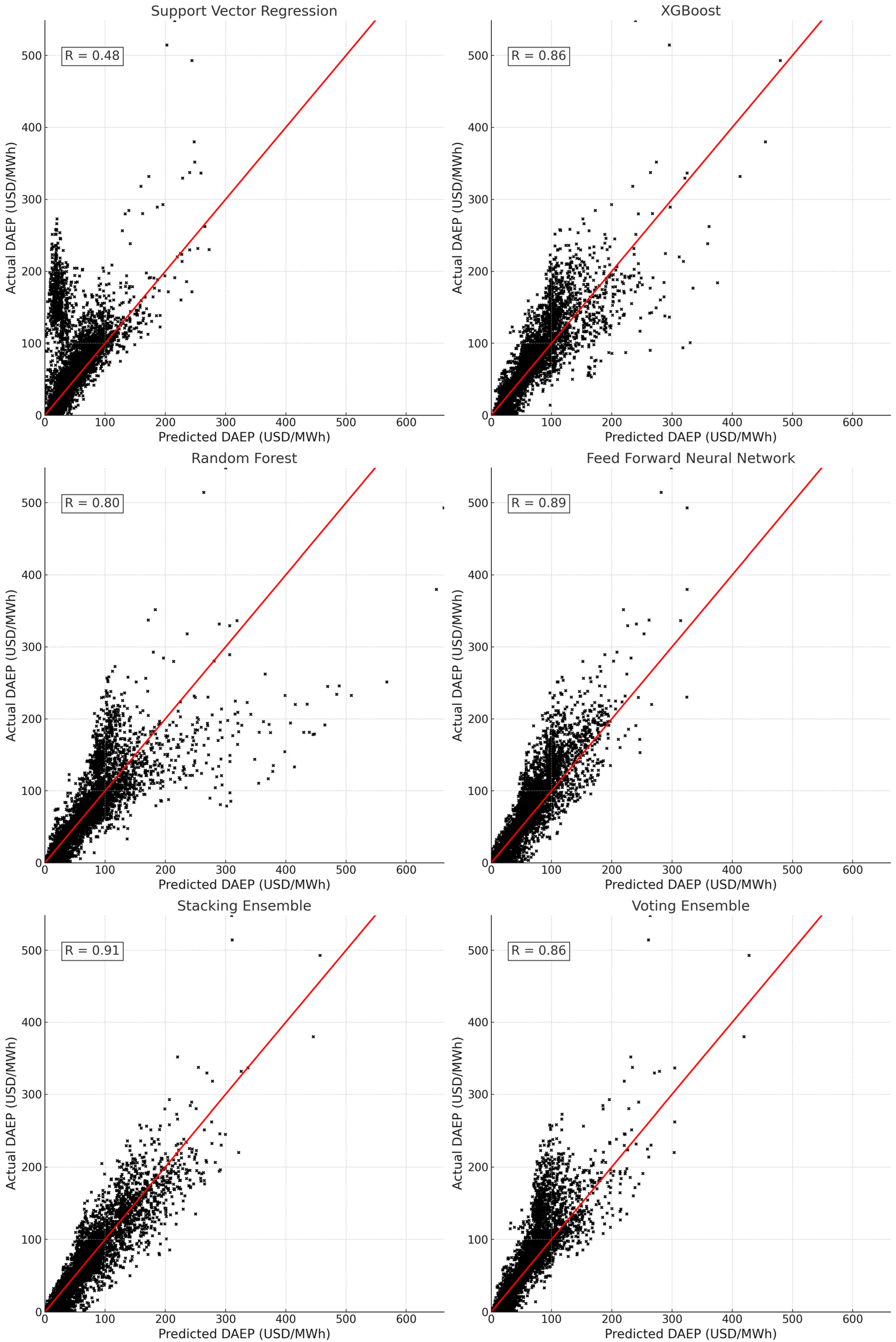
The hourly datasets, encompassing the DAEP, real-time market prices, and actual and forecasted load and forecasted wind values, were sourced from the California Independent System Operator (CAISO) [33] from 1 January 2017 to 31 July 2023. The processed hourly data are made publicly available in the data availability section. Additional predictors, outlined in

Table 1. Predictors used in the DAEP forecast model at time $t+24$ (i.e., the 24-hour forecast horizon).

Predictor	Explanation
Wind_forecast	Forecasted wind generation for $t+24$, available during the forecast
Load_forecast	Forecasted electricity demand for $t+24$, available during the forecast
Real_time_price_lag24	Real-time electricity price (USD/MWh) from $t-24$
Hour	Hour of the day (0–23) at $t+24$, indicating daily cyclical patterns
Day_of_week	Day of the week (0–6, Monday–Sunday) at $t+24$, capturing weekly cycles
Month	Month at $t+24$, capturing seasonal cycle
Is Holiday Target	Binary indicator (1 if $t+24$ is a U.S. federal holiday, 0 otherwise) reflecting holiday effects
Load_actual_lag24	Actual electricity demand (MW) from $t-24$
Lag_1h	Day-ahead price (USD/MWh) from $t-1$, capturing short-term price trends
Lag_24h	Day-ahead price (USD/MWh) from $t-24$, reflecting daily price persistence
Moving_avg_3h	3 h moving average of day-ahead prices up to $t-1$, smoothing short-term fluctuations
Moving_avg_6h	6 h moving average of day-ahead prices up to $t-1$, capturing intraday trends
Moving_avg_12h	12 h moving average of day-ahead prices up to $t-1$, reflecting half-day patterns
Moving_avg_24h	24 h moving average of day-ahead prices up to $t-1$, indicating daily trends
Moving_avg_7d	7-day moving average of day-ahead prices up to $t-1$, capturing weekly trends
Moving_avg_30d	30-day moving average of day-ahead prices up to $t-1$, smoothing long-term variations
Price_diff_1h	Difference in day-ahead prices between $t-1$ and $t-2$, measuring short-term changes
Price_diff_24h	Difference in day-ahead prices between $t-1$ and $t-25$, capturing daily price shifts

, include engineered endogenous features, such as lagged DAEP prices, moving averages, U.S. federal holiday, and target-time indicators (hour, day of week, and month), designed to capture the diverse temporal dynamics of the DAEP, including short- and long-term trends and market shocks essential for accurate forecasting.

From Table 1, lagged features like Lag_1h and Lag_24h capture autocorrelation, a key aspect of energy price time series, where recent and daily patterns influence future prices. Price differences, Price_diff_1h and Price_diff_24h detect short-term price dynamics, enabling the model to respond to sudden shifts driven by supply-demand imbalances. Therefore, the inclusion of price differences captures short-term market volatility and abrupt price shocks in electricity markets, which often arise from sudden imbalances in supply and demand, such as unexpected outages in renewable generation (e.g., wind or solar), demand spikes due to weather events, or unforeseen grid constraints like transmission line failures. To account for daily patterns and recent market conditions, Real_time_price_lag24 was incorporated as an input feature. This allows the model to learn from recurring intraday trends that often influence both day-ahead and real-time price movements. Time-based features, including hour of the day, day of the week, and month of the target variable (i.e., during the forecast horizon), address daily, weekly, and seasonal cycles prevalent in energy markets, such as evening peak demand or winter price surges. These time variables were cyclically encoded using sine and cosine transformations to preserve their periodic nature: hour of the day over a 24 h cycle (to create hour_sin, hour_cos), day of the week over a 7-day cycle (to create day_of_week_sin, day_of_week_cos), and month over a 12-month cycle (to create month_sin, month_cos), with months adjusted from 1–12 to 0–11. This two-dimensional encoding ensures a continuous time representation, allowing the DAEP forecasting model to learn temporal patterns effectively. Moving averages (Moving_avg_3h to Moving_avg_30d), spanning windows from 3 h to 30 days, smooth out noise and reveal trends, were calculated using Equation (1) and shifted accordingly to avoid look-ahead bias.

$$M{A}_t^{\left(w\right)}={\displaystyle \frac{1}{w}}{\sum }_{i=0}^{w-1}{Y}_{t-i}$$

(1)

$M{A}_t^{\left(w\right)}$ is the moving average at the time $t$ over a window $w$ (e.g., 3 h to 30 days), and $Y_{t-i}$ are the DAEP values from the previous $w$ hours.

Figure 1 illustrates the DAEP forecasting workflow using the predictors from Table 1. The methodology comprises two tasks. Task 1 implements a 2372-day, 24 h rolling window cross-validation with XGBoost to robustly evaluate forecasts, adapting to evolving market conditions across the dataset. Task 2 simulates a real-life scenario, forecasting the DAEP for 31 July 2023, based on a runtime of 10 AM on 30 July 2023, and assesses model uncertainty by comparing RF, SVR, XGBoost, FFNN [34], voting, and stacking ensemble methods. Additionally, Task 2 employs a train–test split (training up to 31 December 2022 and testing from 1 January to 31 July 2023) to evaluate performance over an extended period beyond a single-day forecast, providing a comprehensive analysis of model robustness and uncertainty under different validation scenarios.

From Figure 1, Task 1 involves a 7-day training window to capture recent trends and a 24 h step size to simulate daily forecasting, mirroring real-world conditions. The cross-validation approach employs a custom 24 h rolling window to sequentially split the full dataset from 1 January 2017 00:00 to 31 July 2023 23:00, training on historical data and validating on the subsequent 24 h period. This ensures a 24 h lead time forecast across diverse market scenarios, such as peak demand, holidays, or weather-driven volatility. In the next step, SHAP evaluates the contribution of each predictor in Table 1, providing insight into their relevance for DAEP forecasting. SHAP, a game-theoretic approach, assigns each feature an importance value based on its contribution to the model’s output, adeptly handling non-linearities, multicollinearity, and interactions among predictors [35]. To achieve this, SHAP uses the Shapley value from cooperative game theory to fairly distribute the model’s prediction across predictors. In energy price forecasting, SHAP helps stakeholders understand which factors most influence predictions, aiding decision-making by ranking predictors that are most influential for forecasting the DAEP with a 24 h lead time, thereby offering a global assessment of market-relevant factors.

In Task 2, to simulate a real-world scenario of forecasting the DAEP with a 24 h lead time at a runtime with available historical and forecast data, XGBoost, RF, FFNN, and SVR models were trained until runtime and tested. For the runtime scenario at 10 a.m. on 30 July 2023, the models were trained on data from 1 January 2017 00:00 to 30 July 2023 09:00 and used to forecast the DAEP for 31 July 2023, 00:00 to 23:00. To assess model performance over a broader period and draw robust conclusions, the dataset was also split into a train/validation set (1 January 2017 00:00 to 31 December 2022 23:00, with 70% for training and 30% for validation) and a test set (1 January 2023 00:00 to 31 July 2023 23:00). Optimal hyperparameters were objectively selected using GridSearchCV with TimeSeriesSplit from scikit-learn [36] for XGBoost, RF, and SVR, preserving temporal order and preventing data leakage. For FFNN, hyperparameters were objectively optimized using KerasTuner’s Random Search [37]. In each case, the optimal combination of parameters that minimizes the validation loss was selected. Table S1 contains the details on the tuned hyperparameters for each model. Model performance was evaluated with Mean Absolute Error (MAE) [38], measuring average absolute error in USD and robust to outliers, and Root Mean Squared Error (RMSE) [38], which penalizes larger errors for a comprehensive accuracy assessment across volatile DAEP data. To leverage the complementary strengths of the individual models, a stacking ensemble [39] was implemented. Predictions from RF, SVR, XGBoost, and FFNN base models were generated on the validation set (January–April 2023) and combined using a linear regression meta-model. This meta-model was trained to optimize weights for each base model’s predictions, aiming to enhance overall accuracy beyond any single model. Additionally, an averaging ensemble (henceforth referred to as ‘voting’, with each model having equal weight) was applied by computing the arithmetic mean of predictions from all base models, capitalizing on their collective predictive power to reduce variance and improve robustness.

3. Results

Figure 2 presents a scatter plot that evaluates the performance of the XGBoost model in forecasting the DAEP across a comprehensive 2372-day period, utilizing a 24 h rolling window. Figure 2 compares the actual DAEP values (in USD/MWh) against the predicted DAEP values, depicting the model’s predictive accuracy across various market conditions. The model’s performance metrics are notably robust, with a median MAE of 6.26 USD/MWh and RMSE of 8.27 USD/MWh across the 2372 evaluation folds. These metrics suggest a high level of forecast accuracy in 24 h of lead time, particularly for DAEP values falling within the 0–700 USD/MWh range, where most of the data points are concentrated. The tight clustering of points around the red regression line in this range indicates that the XGBoost model effectively captures the underlying patterns and trends in the day-ahead energy market during periods of relative stability. However, the scatter plot also reveals limitations in the model’s forecasting ability as the DAEP values increase beyond 700 USD/MWh. The data points in these higher ranges, which often correspond to periods of heightened market volatility—such as during extreme weather events, supply disruptions, or sudden demand spikes—deviate more significantly from the regression line. This suggests that the model struggles to predict larger DAEP values accurately, where market dynamics become more complex and less predictable.

Table 2. Summary statistics of the day-ahead energy price during the analysis period.

Statistic	USD/MWh
Mean	50.5
Standard Deviation	55.27
25th Percentile	26.62
50th Percentile	37.72
75th Percentile	58.15
99th Percentile	269.92
Maximum	1577.51

presents the DAEP summary statistics during the analysis period. The majority of DAEP values range between approximately 26.62 USD/MWh and 58.15 USD/MWh (25th to 75th percentile), with a mean of 50.05 USD/MWh and a standard deviation of 55.27 USD/MWh, which the XGBoost model in Figure 2 forecasts relatively more accurately (Figure 2). However, extreme price fluctuations are evident, with a minimum of −19.24 USD/MWh and a maximum of 1577.51 USD/MWh, highlighting significant market volatility. These sharp deviations indicate challenges in forecasting, as sudden price spikes and negative pricing events suggest high sensitivity to supply–demand imbalances, regulatory factors, and external shocks. Therefore, the XGBoost model’s strength lies in its ability to learn from historical data and identify linear and non-linear relationships, which serves it well under normal market conditions.

The SHAP analysis showed that predictors such as US federal holidays achieved 0 SHAP values and were removed from the model. The SHAP analysis in Figure 3a provides insight into the feature importance driving the XGBoost model’s predictions of the DAEP, as illustrated in Figure 2. This analysis reveals that historical price lags are the most influential predictors, with the previous hour’s DAEP (lag_1h) exhibiting the highest mean SHAP value, indicating a substantial impact on the model output with a contribution of approximately 12.99 units (i.e., 25.01% of the total contribution). The same hour from the previous day (lag_24) follows closely, contributing around 9.37 units (i.e., 18.10% of the total contribution), highlighting the market’s reliance on short-term and daily recurrent price trends. These findings highlight the inertial nature of energy markets, where recent price movements and diurnal patterns, driven by consistent demand cycles such as morning and evening peaks, play a pivotal role in shaping day-ahead pricing. Engineered features, like the 30-day moving average (moving_avg_30d), contributed moderately, with 3.01 units, i.e., 5.82% contribution, capturing longer-term trends that reflect gradual shifts in market conditions, such as seasonal demand variations or supply availability. Cyclical features, encoded using sine and cosine transformations, further enhance the model’s temporal sensitivity. Sine components, including day_of_week_sin (approximately 2.92 units and 5.63% contribution), hour_sin (approximately 2.21 units and 4.27% contribution), and month_sin (1.26 units and 2.34% contribution), outperform their cosine counterparts (day_of_week_cos, hour_cos, month_cos), suggesting a stronger alignment with peak demand periods, such as midweek for day_of_week_sin, evening hours for hour_sin, and seasonal extremes for month_sin, that drive significant price fluctuations. Additional features, such as price_diff_24h (approximately 2.91 units and 5.63% contribution), load_forecast (approximately 2.23 units and 4.31% contribution), and real_time_price_lag24 (approximately 2.23 units and 4.30% contribution), contribute to detecting short-term shocks, forward-looking demand signals, and immediate supply–demand imbalances, respectively, adding to the model’s predictive capability.

The SHAP summary plot in Figure 3b complements these findings by illustrating the direction and magnitude of each feature’s impact on the model output. The plot shows that lag_1h and lag_24 consistently exert a positive influence on DAEP predictions, with SHAP values extending into the positive range (up to 500 units), indicating that upward price movements in the immediate past strongly correlate with higher day-ahead prices. Cyclical features, like hour_sin and day_of_week_sin, also show positive SHAP values during peak demand periods (e.g., evening hours or midweek), reinforcing their role in capturing demand-driven price spikes. The spread of SHAP values for these features, marked by red (high feature values) and blue (low feature values), reveals a broad range of impacts, suggesting that the model adapts to varying market conditions. In contrast, features like price_diff_1h and wind_forecast exhibit more balanced positive and negative impacts, with SHAP values ranging from −100 to +200 units, reflecting their sensitivity to short-term volatility and renewable energy supply fluctuations. The lower contributions of shorter-term moving averages (e.g., moving_avg_3h, moving_avg_6h) and cosine components (e.g., month_cos) indicate diminishing returns in capturing rapid changes within those timeframes or transitional phases, as energy prices are more responsive to peak demand events than gradual shifts.

The evaluation of model uncertainty in forecasting the DAEP for varying lead times, as part of Task 2 (Figure 1), is a critical aspect of understanding the reliability of predictive models in the dynamic context of energy markets. Figure 4 illustrates the performance of several machine learning models, including XGBoost, FFNN, RF, and SVR, in forecasting the DAEP for the 24 h period on 31 July 2023, with predictions generated at 10:00 a.m. on 30 July 2023. These forecasts leverage the historical predictor data detailed in Figure 3, which includes features such as lagged prices, cyclical patterns, and load forecasts, providing a foundation for capturing market trends. Figure 4 shows that all models demonstrate promising results in capturing the diurnal DAEP profile, which reflects the typical demand cycles in the energy market. The prices gradually increased in the morning, peaking around noon due to heightened daytime industrial and commercial activity, and reaching a maximum at 7:00 p.m. as residential demand surges during evening hours. This peak is followed by a sharp decline into the late evening and night, consistent with reduced consumption as businesses close and households scale back usage (Figure 4). This pattern aligns with the natural rhythm of electricity demand, influenced by weather, economic activity, and consumer behavior. These are critical drivers in day-ahead markets where prices are set 24 h in advance based on anticipated supply and demand. The ability of the models to trace this trend highlights their effectiveness in leveraging historical and cyclical features to predict short-term price movements.

Among the individual models, SVR emerges as the top performer, achieving an MAE of 7.48 USD/MWh and an RMSE of 10.24 USD/MWh. These metrics indicate a high level of accuracy, particularly in capturing the details of the diurnal peak, suggesting that SVR’s kernel-based approach excelled in the test period (31 July 2023) at modeling the non-linear relationships inherent in energy price data. XGBoost follows with an MAE of 12.62 USD/MWh and an RMSE of 17.14 USD/MWh, random forest follows with an MAE of 13.14 USD/MWh and an RMSE of 20.94 USD/MWh, and FFNN follows with an MAE of 16.22 USD/MWh and an RMSE of 20.00 USD/MWh.

The ensemble techniques provide an additional layer of analysis, combining predictions from the base models to potentially enhance accuracy. The voting ensemble, which averages the forecasts from individual models, achieves an MAE of 12.37 USD/MWh and an RMSE of 17.08 USD/MWh, performing closely to XGBoost but falling short of SVR’s precision. This suggests that the averaging process smooths out some errors but does not fully capitalize on the strengths of the best-performing model. The stacking ensemble, which employs a meta-model of linear regression trained on base model forecasts validated from January 2023 to April 2024, yields an MAE of 13.49 USD/MWh and an RMSE of 21.04 USD/MWh. This relatively higher error indicates that, in the test period, the linear meta-model may not have adequately captured the non-linear dynamics present in the data, particularly during the rapid price ascent and descent around the 7:00 p.m. peak, where the stacking approach appears to underestimate volatility.

The final assessment of model performance in forecasting the DAEP with a 24 h lead time is presented in Figure 5, which showcases scatter plots comparing predicted versus actual DAEP values from 1 January 2023 to 31 July 2023 across multiple models and ensemble techniques. This analysis further evaluates the models’ predictive capabilities over a diverse seven-month timeframe, reflecting varying market conditions, such as seasonal demand shifts, weather impacts, and supply fluctuations typical of energy markets. The scatter plots, featuring a red regression line for each model, reveal the alignment between predicted and actual DAEP values, with the density of points around the line indicating the model’s accuracy. This extended evaluation period allows for a robust assessment of how well each model captures the relationship of historical price lags, cyclical patterns, and exogenous factors like load forecasts, which are critical drivers in day-ahead electricity markets.

Among the ensemble techniques, the stacking ensemble emerges as the top performer, achieving an MAE of 15.86 USD/MWh and an RMSE of 23.33 USD/MWh within the notable volatile period of DAEP values exceeding 500 USD/MWh. This superior performance is attributed to its meta-model approach, which leverages linear regression to combine predictions from base models (XGBoost, random forest, FFNN, and SVR), validated over a broad dataset (i.e., 30% of the training data from 1 January 2017 to 31 December 2022), thereby smoothing out individual model biases and capturing a wider range of market behaviors. In contrast, the voting ensemble, which averages predictions from the same base models, trails with an MAE of 18.82 USD/MWh and an RMSE of 31.11 USD/MWh, suggesting that a simple averaging approach in this case diluted the precision of the best-performing models during periods of high volatility. Among the individual models, XGBoost leads with an MAE of 17.95 USD/MWh and an RMSE of 28.58 USD/MWh, followed by RF with an MAE of 20.11 USD/MWh and an RMSE of 35.89 USD/MWh, while FFNN records an MAE of 18.83 USD/MWh and an RMSE of 30.99 USD/MWh.

These results highlight the variability in model performance across different training and test scenarios, a critical consideration in the real-world application of DAEP forecasting. The shift in the best-performing model from SVR in Figure 4 (MAE: 7.48 USD/MWh, RMSE: 10.24 USD/MWh for a specific 24 h period on 31 July 2023) to the stacking ensemble in Figure 5 over a longer timeframe indicates that relying on a static test period or a single model is non-optimal.

4. Discussion

The California Independent System Operator (CAISO) energy market, characterized by high renewable energy integration, exhibits significant volatility driven by weather patterns, demand fluctuations, and regulatory dynamics [40]. This study focused on Day-Ahead Energy Price (DAEP) forecasting within this complex market, spanning from January 2017 to July 2023, during which the DAEP displayed a mean of 50.05 USD/MWh and a standard deviation of 55.27 USD/MWh (Table 1), reflecting considerable volatility. Previous studies have shown that DAEP forecast errors vary depending on the model choice and evaluation periods [41,42]. For instance, ref. [43] reported MAEs ranging from 4.9 to 10 USD/MWh across models for CAISO data between January 2017 and December 2018. Our study, employing a 24 h lead time forecast and a robust evaluation framework with a 24 h rolling window validated across 2372 folds, achieved a competitive median MAE of 6.26 USD/MWh and RMSE of 8.27 USD/MWh using XGBoost. Cross-validation ensured a comprehensive 24-hour assessment across diverse market conditions, contrasting with the static test periods often used in prior DAEP studies [44,45].

A key strength of this study is its advanced feature selection process, utilizing SHapley Additive exPlanations (SHAP) to identify and prioritize predictors capturing hourly, daily, weekly, and monthly cyclic patterns in CAISO’s DAEP data (Figure 3). Top engineered features, including the previous hour’s DAEP (25.10% SHAP contribution), same-hour DAEP from the previous day (18.10%), and features like moving averages and sine-based cyclical indicators enhanced the models’ ability to reflect inherent periodicities and seasonality. These findings align with refs. [46,47], who used SHAP to emphasize feature selection in DAEP forecasting, and [43], who highlighted the dominance of historical DAEP lags over exogenous features in CAISO. However, during highly volatile periods, the model struggled to capture DAEP spikes (Figure 2), indicating the need for reliable exogenous variables, such as weather data and market policies, to better address price shocks [48,49].

To mirror real-world scenarios, runtime forecasts at 10 AM on the prior day provided a practical evaluation of model performance, revealing the necessity of ensemble forecasting to combine the strengths of individual models. The runtime approach reflects CAISO’s operational demands, where emergent patterns, such as sudden renewable generation drops, may favor one model (e.g., SVR in Figure 4, MAE 7.48 USD/MWh on 31 July 2023) over another in a different period (e.g., stacking ensemble in Figure 5, MAE 15.86 USD/MWh over seven months). Energy markets evolve with factors like demand spikes, extreme weather, renewable integration, and regulatory shifts [50]. Therefore, relying on a static train–test split to determine a single best model can be misleading [51]. Instead, forecasting with an ensemble of models across varied market conditions and assessing ensemble spread in bidding decisions offer a more robust approach. The focus on ensemble methods and scenario-specific validation beyond a single train–test split supports scalable, adaptable forecasting models that leverage individual strengths (e.g., SVR’s non-linear modeling, XGBoost’s feature handling, neural networks’ complex interactions) without a singular conclusion, fitting the dynamic nature of CAISO.

Considering that the goal of enhancing DAEP forecasting is to optimize bidding decisions, enabling market participants to decide between selling in the day-ahead or real-time market [52], it is essential to extend the framework presented in Figure 1 to include real-time price forecasting in the same runtime and compare DAEP and real-time price forecasts to inform bidding decisions [53]. Figures S1 and S2 demonstrate that the framework developed in this study is capable of achieving this by forecasting the DAEP on 10 April 2023 (a U.S. holiday) and comparing it with the real-time price forecast (mirroring the predictors in Table 1 but with real-time price as the target) to enhance bidding decisions. The stacking ensemble achieved the lowest error, with an MAE of 16.47 USD/MWh, despite the holiday’s unique cyclic patterns. This suggests that the model applies to days with special events, such as holidays. The bidding decisions achieved an accuracy of 83.3%, correctly identifying hours when the DAEP was either greater than or less than the real-time price. These findings form the foundation for developing the EnergyBidMaster (the web app (EnergyBidMaster) developed with the Python codes from this study for smart bidding in energy markets is available at https://energybidmaster.com/, accessed on 3 April 2025) web application that applied an ensemble of ML models for smart bidding. Hence, this study provides a foundation that improves DAEP forecasting accuracy and supports strategic bidding decisions under varying market conditions, including holidays and other special events.

A limitation of this study is its reliance on engineered endogenous features, which excel in CAISO when the DAEP ranges from 0 to 700 USD/MWh (Figure 2) but struggle with extreme volatility. Therefore, considering that the difference between predicted and actual prices is usually small in the specified range, the choice of forecasting method is less critical, with limited impact on market operations. Once price fluctuations exceed a certain critical threshold (e.g., 700 USD/MWh for this study, Figure 2), prediction errors can grow significantly, leading to price spikes (i.e., large price deviations) and potentially compromising power system security and stability. Thus, more careful selection and rigorous validation of forecasting methods are necessary under these conditions. While the ML framework in this study (Figure 1) advances feature engineering, incorporating exogenous features, like real-time weather data or market sentiment indicators, could address these gaps. Future research should explore enhancements to improve DAEP forecasting accuracy in volatile periods.

5. Conclusions

This study forecasted Day-Ahead Energy Prices (DAEP) from the California Independent System Operator (CAISO) market with a 24 h lead time, focusing on (1) comprehensive feature engineering with endogenous features capturing daily, weekly, and seasonal cyclic patterns; (2) enhanced feature selection and interpretability using SHAP; (3) model forecast uncertainty evaluation and the added value of ensemble techniques; and (4) comprehensive forecast evaluation using cross-validation, runtime forecasting at 10 a.m., and a static train–test split. The major conclusions are as follows:

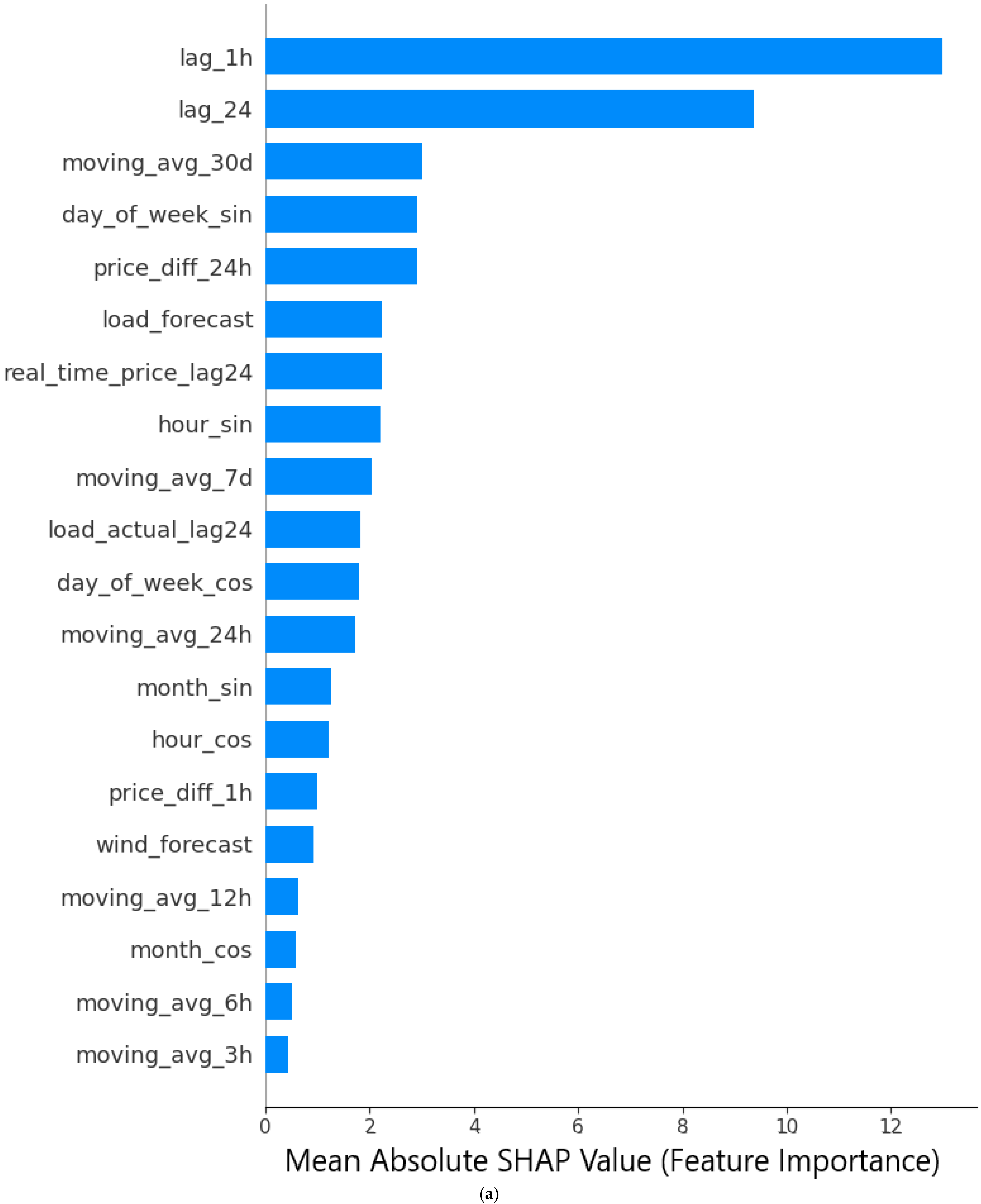
• SHAP analysis identified endogenous features, including the DAEP from 1 h ago, 24 h ago, 30-day moving average, day of the week, and DAEP difference between t − 1 and t − 25, as top contributors, driving approximately 60% of model accuracy.
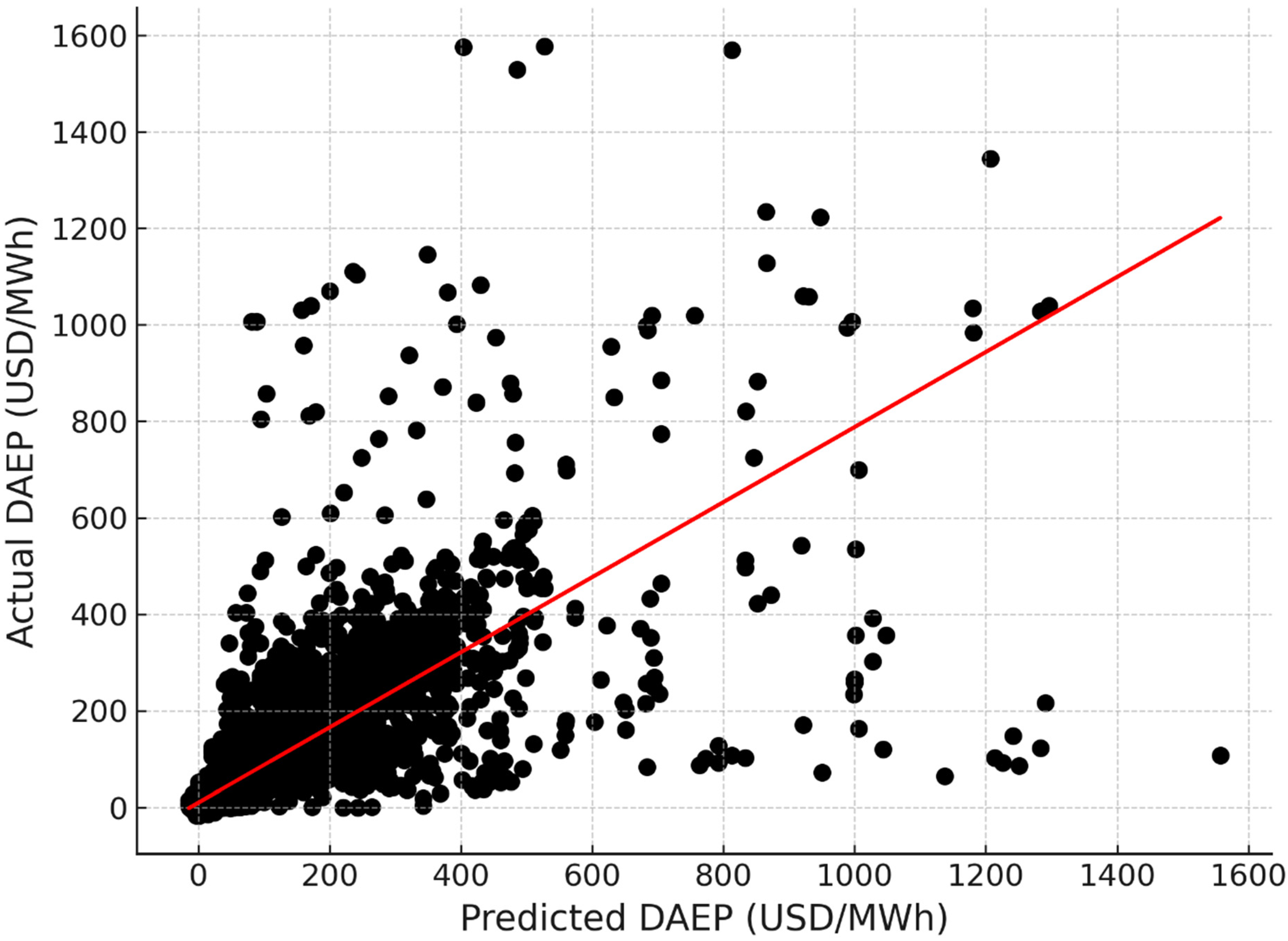
• XGBoost cross-validation across 2372-day folds with a 24 h rolling window achieved a median MAE of 6.26 USD/MWh and RMSE of 8.27 USD/MWh across a highly volatile analysis period.
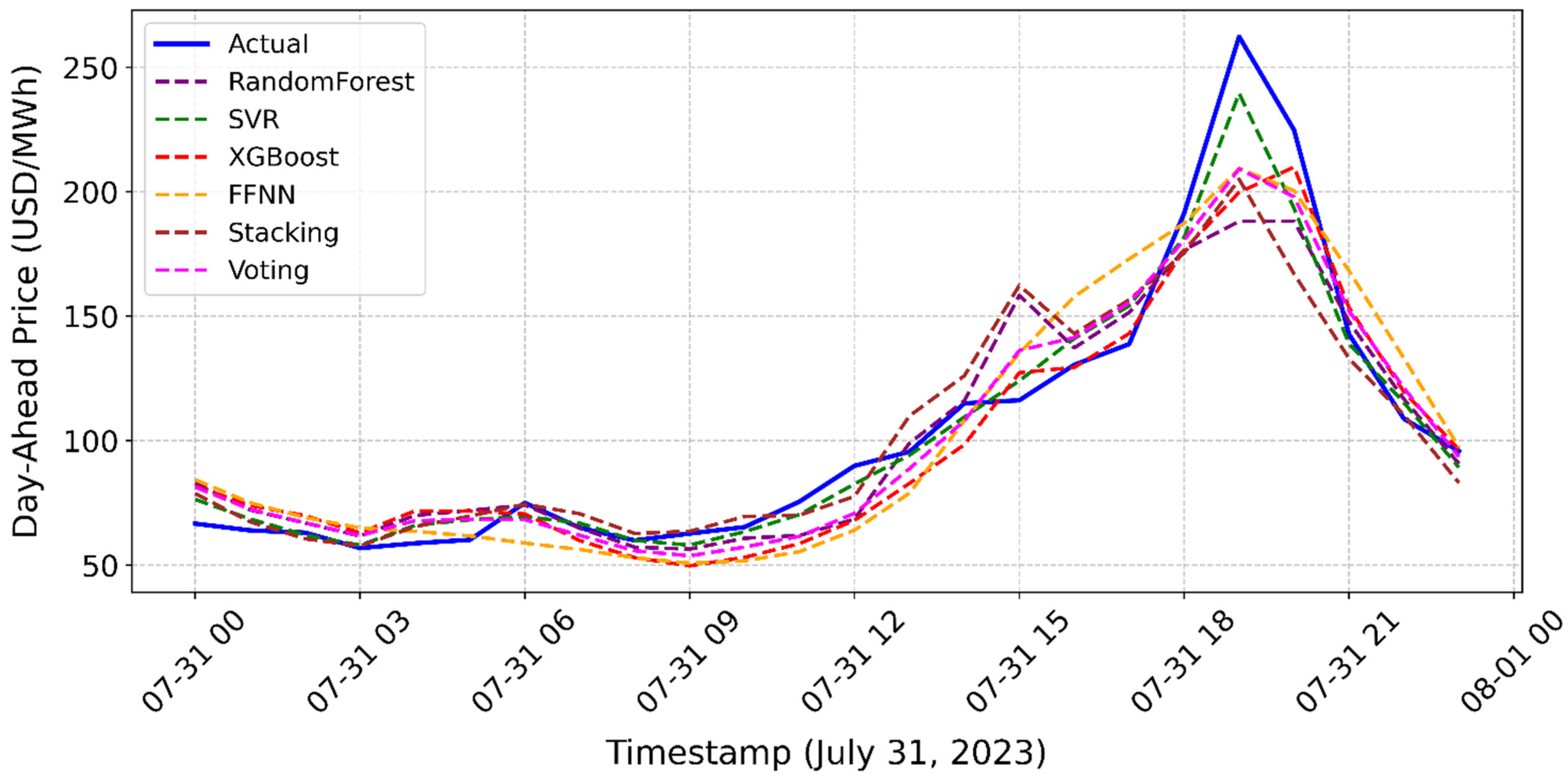
• The best-performing model varies by forecast model, training period, and test period, highlighting the need for ensemble forecasting using multiple models (e.g., SVR, XGBoost, RF, FFNN), combining the strengths of base models through methods such as voting and stacking, and using a dynamic evaluation period to capture different market conditions.

References

1. Hassan, Q.; Viktor, P.; Al-Musawi, T.J.; Ali, B.M.; Algburi, S.; Alzoubi, H.M.; Al-Jiboory, A.K.; Sameen, A.Z.; Salman, H.M.; Jaszczur, M. The renewable energy role in the global energy Transformations. Renew. Energy Focus 2024, 48, 100545. [Google Scholar] [CrossRef]
2. Safari, A.; Gharehbagh, H.K.; Nazari-Heris, M.; Zare, K. Design of a Dynamic Feedback LSTM Electricity Price Forecast of Smart Grids. In Artificial Intelligence in the Operation and Control of Digitalized Power Systems; Springer Nature: Cham, Switzerland, 2024; pp. 327–344. [Google Scholar]
3. Cheng, L.; Huang, P.; Zhang, M.; Yang, R.; Wang, Y. Optimizing Electricity Markets Through Game-Theoretical Methods: Strategic and Policy Implications for Power Purchasing and Generation Enterprises. Mathematics 2025, 13, 373. [Google Scholar] [CrossRef]
4. Abidi, I.; Nsaibi, M. Assessing the impact of renewable energy in mitigating climate change: A comprehensive study on effectiveness and adaptation support. Int. J. Energy Econ. Policy 2024, 14, 442–454. [Google Scholar] [CrossRef]
5. Strielkowski, W.; Civín, L.; Tarkhanova, E.; Tvaronavičienė, M.; Petrenko, Y. Renewable energy in the sustainable development of electrical power sector: A review. Energies 2021, 14, 8240. [Google Scholar] [CrossRef]
6. Constante, D.M.A.; Erazo, C.R.R. The role of renewable energies in the transition to a sustainable energy model: Challenges and opportunities. J. Bus. Entrep. Stud. 2024, 8, 38–48. [Google Scholar]
7. Hassan, W.; Elsabbagh, B.; Abdelaziz, A.; Essam, G.; Aboushama, R. Energy Trading Enhancing Sustainability. In Artificial Intelligence and Machine Learning for Sustainable Development: Innovations, Challenges, and Applications; CRC Press: Boca Raton, FL, USA, 2024; p. 33. [Google Scholar]
8. Coker, P.J.; Bloomfield, H.C.; Drew, D.R.; Brayshaw, D.J. Interannual weather variability and the challenges for Great Britain’s electricity market design. Renew. Energy 2020, 150, 509–522. [Google Scholar] [CrossRef]
9. Gonçalves, A.C.; Costoya, X.; Nieto, R.; Liberato, M.L. Extreme weather events on energy systems: A comprehensive review on impacts, mitigation, and adaptation measures. Sustain. Energy Res. 2024, 11, 4. [Google Scholar] [CrossRef]
10. Kumar, R.R.; Sanjai, M.; Sivashanmugam, R.; Saranya, S.; Sinega, S.; Logeswaran, T. Grid integration of renewable energy sources with IoT system. In Proceedings of the 2022 International Conference on Sustainable Computing and Data Communication Systems (ICSCDS), Erode, India, 7–9 April 2022; pp. 1012–1017. [Google Scholar]
11. Medina, C.; Ana, C.R.M.; González, G. Transmission grids to foster high penetration of large-scale variable renewable energy sources–A review of challenges, problems, and solutions. Int. J. Renew. Energy Res. 2022, 12, 146–169. [Google Scholar]
12. Foster, J.M. Control Systems in Power Markets: Demand Response, Transmission Topology Control, and Renewable Integration. Ph.D. Thesis, Boston University, Boston, MA, USA, 2012. [Google Scholar]
13. Welton, S. Electricity markets and the social project of decarbonization. Columbia Law Rev. 2018, 118, 1067–1138. [Google Scholar]
14. Ketterer, J.C. The impact of wind power generation on the electricity price in Germany. Energy Econ. 2014, 44, 270–280. [Google Scholar] [CrossRef]
15. Van Kuik, G.A.M.; Peinke, J.; Nijssen, R.; Lekou, D.; Mann, J.; Sørensen, J.N.; Ferreira, C.; van Wingerden, J.W.; Schlipf, D.; Gebraad, P.; et al. Long-term research challenges in wind energy—A research agenda by the European Academy of Wind Energy. Wind. Energy Sci. 2016, 1, 1–39. [Google Scholar] [CrossRef]
16. Aderibigbe, A.O.; Ani, E.C.; Ohenhen, P.E.; Ohalete, N.C.; Daraojimba, D.O. Enhancing energy efficiency with ai: A review of machine learning models in electricity demand forecasting. Eng. Sci. Technol. J. 2023, 4, 341–356. [Google Scholar] [CrossRef]
17. Ibebuchi, C.C.; Richman, M.B. Deep learning with autoencoders and LSTM for ENSO forecasting. Clim. Dyn. 2024, 62, 5683–5697. [Google Scholar] [CrossRef]
18. Allal, Z.; Noura, H.N.; Salman, O.; Chahine, K. Machine learning solutions for renewable energy systems: Applications, challenges, limitations, and future directions. J. Environ. Manag. 2024, 354, 120392. [Google Scholar] [CrossRef]
19. Rane, N.L.; Choudhary, S.P.; Rane, J. Artificial Intelligence and machine learning in renewable and sustainable energy strategies: A critical review and future perspectives. Partn. Univers. Int. Innov. J. 2024, 2, 80–102. [Google Scholar] [CrossRef]
20. Wegener, C.; Ibebuchi, C.C. Application of XGBOOST in Disentangling the Fingerprints of Global Warming and Interdecadal Pacific Oscillation on Seasonal Precipitation Trends in Ohio. Res. Sq. 2024. [Google Scholar] [CrossRef]
21. Awad, M.; Khanna, R.; Awad, M.; Khanna, R. Support vector regression. In Efficient Learning Machines: Theories, Concepts, and Applications for Engineers and System Designers; Apress: Berkeley, CA, USA, 2015; pp. 67–80. [Google Scholar]
22. Breiman, L. Random forests. Mach. Learn. 2001, 45, 5–32. [Google Scholar] [CrossRef]
23. Manohar, V.J.; Murthy, G.; Royal, N.P.; Binu, B.; Patil, T. Comprehensive Analysis of Energy Demand Prediction Using Advanced Machine Learning Techniques. In Proceedings of the 2nd International Conference on Renewable Energy, Green Computing and Sustainable Development (ICREGCSD 2025), Hyderabad, India, 21–22 February 2025; Volume 616, p. 02027. [Google Scholar]
24. Xie, H.; Chen, S.; Lai, C.; Ma, G.; Huang, W. Forecasting the clearing price in the day-ahead spot market using eXtreme Gradient Boosting. Electr. Eng. 2022, 104, 1607–1621. [Google Scholar] [CrossRef]
25. Tschora, L.; Pierre, E.; Plantevit, M.; Robardet, C. Electricity price forecasting on the day-ahead market using machine learning. Appl. Energy 2022, 313, 118752. [Google Scholar] [CrossRef]
26. Tan, Y.Q.; Shen, Y.X.; Yu, X.Y.; Lu, X. Day-ahead electricity price forecasting employing a novel hybrid frame of deep learning methods: A case study in NSW, Australia. Electr. Power Syst. Res. 2023, 220, 109300. [Google Scholar] [CrossRef]
27. Sun, C.; Pan, X.; Li, G.; Li, P.; Gao, G.; Tian, Y.; Xu, G. Day-Ahead Electricity Price Forecasting Strategy Based on Machine Learning and Optimization Algorithm. In Proceedings of the 2022 4th Asia Energy and Electrical Engineering Symposium (AEEES), Chengdu, China, 25–28 March 2022; pp. 254–259. [Google Scholar]
28. Bae, D.J.; Kwon, B.S.; Song, K.B. XGBoost-based day-ahead load forecasting algorithm considering behind-the-meter solar PV generation. Energies 2021, 15, 128. [Google Scholar] [CrossRef]
29. Raviv, E.; Bouwman, K.E.; Van Dijk, D. Forecasting day-ahead electricity prices: Utilizing hourly prices. Energy Econ. 2015, 50, 227–239. [Google Scholar] [CrossRef]
30. Nohara, Y.; Matsumoto, K.; Soejima, H.; Nakashima, N. Explanation of machine learning models using improved shapley additive explanation. In Proceedings of the 10th ACM International Conference on Bioinformatics, Computational Biology and Health Informatics, Niagara Falls, NY, USA, 7–10 September 2019; p. 546. [Google Scholar]
31. Divina, F.; Gilson, A.; Goméz-Vela, F.; García Torres, M.; Torres, J.F. Stacking ensemble learning for short-term electricity consumption forecasting. Energies 2018, 11, 949. [Google Scholar] [CrossRef]
32. Solano, E.S.; Affonso, C.M. Solar irradiation forecasting using ensemble voting based on machine learning algorithms. Sustainability 2023, 15, 7943. [Google Scholar] [CrossRef]
33. California Independent System Operator (CAISO). CAISO Market Data. 2025. Available online: https://www.caiso.com (accessed on 15 February 2025).
34. Ibebuchi, C.C.; Rainey, S.; Obarein, O.A.; Silva, A.; Lee, C.C. Comparison of machine learning models in forecasting different ENSO types. Phys. Scr. 2024, 99, 086007. [Google Scholar] [CrossRef]
35. Sahlaoui, H.; Nayyar, A.; Agoujil, S.; Jaber, M.M. Predicting and interpreting student performance using ensemble models and shapley additive explanations. IEEE Access 2021, 9, 152688–152703. [Google Scholar] [CrossRef]
36. Pedregosa, F.; Varoquaux, G.; Gramfort, A.; Michel, V.; Thirion, B.; Grisel, O.; Blondel, M.; Prettenhofer, P.; Weiss, R.; Dubourg, V.; et al. Scikit-learn: Machine learning in Python. J. Mach. Learn. Res. 2011, 12, 2825–2830. [Google Scholar]
37. O’Malley, T.; Bursztein, E.; Long, J.; Chollet, F.; Jin, H. Keras Tuner. 2019. Available online: https://github.com/keras-team/keras-tuner (accessed on 15 February 2025).
38. Hodson, T.O. Root mean square error (RMSE) or mean absolute error (MAE): When to use them or not. Geosci. Model Dev. Discuss. 2022, 15, 5481–5487. [Google Scholar] [CrossRef]
39. Sharma, N.; Mangla, M.; Mohanty, S.N.; Pattanaik, C.R. Employing stacked ensemble approach for time series forecasting. Int. J. Inf. Technol. 2021, 13, 2075–2080. [Google Scholar] [CrossRef]
40. Nyangon, J.; Akintunde, R. Principal component analysis of day-ahead electricity price forecasting in CAISO and its implications for highly integrated renewable energy markets. Wiley Interdiscip. Rev. Energy Environ. 2024, 13, e504. [Google Scholar] [CrossRef]
41. Cai, M.; Pipattanasomporn, M.; Rahman, S. Day-ahead building-level load forecasts using deep learning vs. traditional time-series techniques. Appl. Energy 2019, 236, 1078–1088. [Google Scholar] [CrossRef]
42. Lago, J.; Marcjasz, G.; De Schutter, B.; Weron, R. Forecasting day-ahead electricity prices: A review of state-of-the-art algorithms, best practices and an open-access benchmark. Appl. Energy 2021, 293, 116983. [Google Scholar] [CrossRef]
43. Nizharadze, N.; Farokhi Soofi, A.; Manshadi, S. Predicting the gap in the day-ahead and real-time market prices leveraging exogenous weather data. Algorithms 2023, 16, 508. [Google Scholar] [CrossRef]
44. Alkawaz, A.N.; Abdellatif, A.; Kanesan, J.; Khairuddin, A.S.M.; Gheni, H.M. Day-ahead electricity price forecasting based on hybrid regression model. IEEE Access 2022, 10, 108021–108033. [Google Scholar] [CrossRef]
45. Zhang, C.; Li, R.; Shi, H.; Li, F. Deep learning for day-ahead electricity price forecasting. IET Smart Grid 2020, 3, 462–469. [Google Scholar] [CrossRef]
46. Caffù, D. Explainable Deep Learning Based Electricity Price Forecasting Through SHAP Values for the Extended Cross-Regional Markets Integration. 2021. Available online: https://www.politesi.polimi.it/handle/10589/201356?mode=simple (accessed on 3 April 2025).
47. Liu, H.; Shen, X.; Tang, X.; Liu, J. Day-Ahead electricity price probabilistic forecasting based on SHAP feature selection and LSTNet quantile regression. Energies 2023, 16, 5152. [Google Scholar] [CrossRef]
48. Kilian, L. The economic effects of energy price shocks. J. Econ. Lit. 2008, 46, 871–909. [Google Scholar] [CrossRef]
49. Lehna, M.; Scheller, F.; Herwartz, H. Forecasting day-ahead electricity prices: A comparison of time series and neural network models taking external regressors into account. Energy Econ. 2022, 106, 105742. [Google Scholar] [CrossRef]
50. Goodell, J.W.; Corbet, S. The evolving landscape of energy finance: Challenges and opportunities during global uncertainty. In Handbook of Financial Integration; Edward Elgar Publishing: Northampton, MA, USA, 2024; pp. 172–191. [Google Scholar]
51. Tan, J.; Yang, J.; Wu, S.; Chen, G.; Zhao, J. A critical look at the current train/test split in machine learning. arXiv 2021, arXiv:2106.04525. [Google Scholar]
52. Ferruzzi, G.; Cervone, G.; Delle Monache, L.; Graditi, G.; Jacobone, F. Optimal bidding in a Day-Ahead energy market for Micro Grid under uncertainty in renewable energy production. Energy 2016, 106, 194–202. [Google Scholar] [CrossRef]
53. Rahimiyan, M.; Baringo, L. Strategic bidding for a virtual power plant in the day-ahead and real-time markets: A price-taker robust optimization approach. IEEE Trans. Power Syst. 2015, 31, 2676–2687. [Google Scholar] [CrossRef]
54. Ibebuchi, C. California Independent System Operator (CAISO) Energy Market Data; Zenodo: Geneva, Switzerland, 2025. [Google Scholar] [CrossRef]
Figure 1. Flow chart of the steps in forecasting day-ahead energy prices.
Forecasting 07 00018 g001
Figure 2. Scatter plot showing the actual and predicted day-ahead energy price across a 2372-day period, utilizing a 24 h rolling window with the XGBoost model.
Forecasting 07 00018 g002
Figure 3. SHAP analysis of global feature importance showing percentage contribution (a) and mean SHAP value of each predictor in Table 1 (b).
Forecasting 07 00018 g003aForecasting 07 00018 g003b
Figure 4. Actual and forecasted DAEP on 31 July 2023, using data available at 10 a.m. runtime on 30 July 2023.
Forecasting 07 00018 g004
Figure 5. Scatter plot showing actual and predicted day-ahead energy price in 24 h lead time across multiple forecast models during the 1 January 2023 to 31 July 2023 test period. Pearson correlation (R) between actual and predicted values is reported in the Figure.
Forecasting 07 00018 g005