Predicting Power Consumption Using Deep Learning with Stationary Wavelet

Abstract

Power consumption in the home has grown in recent years as a consequence of the use of varied residential applications. On the other hand, many families are beginning to use renewable energy, such as energy production, energy storage devices, and electric vehicles. As a result, estimating household power demand is necessary for energy consumption monitoring and planning. Power consumption forecasting is a challenging time series prediction topic. Furthermore, conventional forecasting approaches make it difficult to anticipate electric power consumption since it comprises irregular trend components, such as regular seasonal fluctuations. To address this issue, algorithms combining stationary wavelet transform (SWT) with deep learning models have been proposed. The denoised series is fitted with various benchmark models, including Long Short-Term Memory (LSTM), Gated Recurrent Units (GRUs), Bidirectional Gated Recurrent Units (Bi-GRUs), Bidirectional Long Short-Term Memory (Bi-LSTM), and Bidirectional Gated Recurrent Units Long Short-Term Memory (Bi-GRU LSTM) models. The performance of the SWT approach is evaluated using power consumption data at three different time intervals (1 min, 15 min, and 1 h). The performance of these models is evaluated using metrics such as Root Mean Square Error (RMSE), Mean Absolute Percentage Error (MAPE), and Mean Absolute Error (MAE). The SWT/GRU model, utilizing the bior2.4 filter at level 1, has emerged as a highly reliable option for precise power consumption forecasting across various time intervals. It is observed that the bior2.4/GRU model has enhanced accuracy by over 60% compared to the deep learning model alone across all accuracy measures. The findings clearly highlight the success of the SWT denoising technique with the bior2.4 filter in improving the power consumption prediction accuracy.

1. Introduction

Global electric energy consumption has been on the rise due to economic progress and population growth [1]. The 2019 World Energy Outlook, published by the International Energy Agency, predicts a 2.1% annual increase in worldwide electricity demand until 2040, which is twice the rate of energy production under current policies. This is expected to lead to a rise in total final energy consumption from 19% in 2018 to 24% in 2040 [2]. The housing sector accounts for 27% of the global electricity demand and has a significant impact on overall electricity usage [3]. Anticipating energy consumption is crucial for ensuring a reliable power supply, especially since electricity is used concurrently during power plant production. As a result, numerous predictive models have emerged over the past few decades to forecast building energy consumption [4,5]. In the following discussion, we will explore some of the recently published works in this field.

Forecasting energy consumption is a complex task in time series analysis. Data gathered by smart sensors frequently include redundancy, missing values, outliers, and uncertainties [6], which complicates the prediction of electrical energy usage with conventional methods due to the unpredictable nature of energy consumption trends, including regular seasonal patterns [4,7]. To maximize buildings’ energy efficiency, appropriate operational approaches need to be incorporated into energy control schemes [8]. As a result, a variety of forecasting techniques, including conventional and artificial intelligence (AI) models, have been proposed to address energy consumption prediction. In their review of 116 published studies, Wei et al. [9] identified 128 models for forecasting energy consumption, with 62.48% of them being AI based. Energy consumption forecasting systems can be categorized into statistical models, machine learning models, and hybrid models. Energy consumption forecasting systems can be categorized into statistical models, machine learning models, and hybrid models. Statistical techniques exhibit weaknesses in long-term forecasting and in capturing the non-linear behavior of energy consumption data. In addition, computational methods have shown limited effectiveness in predicting energy demand due to their non-stationary nature and significant trends. Current machine learning approaches are often impacted by overfitting, as dynamic correlations between variables and evolving data characteristics pose challenges. This makes it difficult to ensure long-term reliability when overfitting occurs. Despite their advanced mechanisms for handling long-term dependencies and capturing temporal patterns, Recurrent Neural Networks (RNNs) can still be affected by overfitting. To address these issues and improve prediction accuracy, hybrid models have been proposed. Combining wavelet filtering with deep learning is being investigated to ensure both high-quality input data and optimized data-driven model architectures.

This research not only explores the performance of wavelet-based denoising in improving deep learning model accuracy but also emphasizes the importance of selecting the most suitable mother wavelet for a given dataset. This work makes two notable contributions: First, it employs the biorthogonal wavelet (bior2.4) for its key features, such as perfect reconstruction and symmetry, which make it highly suitable for decomposing electrical data time series. By harnessing these properties, the stationary wavelet transform (SWT) is used to analyze and predict energy consumption patterns. SWT allows for the extraction of valuable insights from different frequency components of the time series data, offering a deeper understanding of both short-term fluctuations and long-term trends in energy usage. Second, Gated Recurrent Units (GRUs), an advanced type of recurrent neural network (RNN), are used to build predictive models. GRU excels at managing sequential data and capturing time-dependent patterns, making it well suited for energy consumption forecasting. Its robustness and efficiency contribute to highly accurate predictions. By combining wavelet-transformed bior2.4 data with GRU-based modeling, significant improvements in forecast accuracy are achieved. The models’ performance is evaluated using real-world data from a benchmark electricity load forecasting dataset, confirming their reliability. The rest of this paper is organized as follows: Section 2 provides an in-depth review of the existing literature. Section 3 explains the algorithms used in the proposed forecasting model. Section 4 details the experimental analysis and results. Finally, Section 5 discusses the outcomes from the real-world dataset, conclusions, and references.

2. Related Works

In this section, we present a state-of-the-art review of the main statistical, machine learning, and hybrid techniques used for predicting electricity power consumption in recent years. In the past, statistical techniques were predominantly employed for the purpose of forecasting energy demand. For instance, in reference [10], Bootstrap aggregating was applied to the autoregressive integrated moving average (ARIMA) and exponential smoothing techniques to predict energy demand across different countries. Additionally, in reference [5], the seasonal autoregressive integrated moving average (SARIMA) model was compared with the neuro-fuzzy model for forecasting electric load. The study in [11] encompassed the application of linear regression (using both single and multiple predictors) as well as quadratic regression models to analyze the hourly and daily energy consumption of a specific household. Moreover, reference [12] introduced the combination of multiple regression and a genetic engineering technique to estimate the daily energy usage of an administration building. However, both approaches were hindered by significant limitations, including the absence of occupancy data and the fact that none of the models were validated for estimating energy usage in similar buildings. In addition, the use of computational methods has demonstrated limited effectiveness in predicting energy demand. Consequently, various prediction models have been experimented with, employing machine learning techniques to enhance forecasting accuracy [13,14,15]. For example, Liu et al. [16] created a support vector machine (SVM) model for forecasting and analyzing energy consumption in public buildings. Leveraging the robust non-linear capabilities of support vector regression, Chen et al. [17] proposed a model for predicting electrical load based on ambient temperature. In addition, energy consumption was predicted by analyzing the collective behavior of population dynamics in [18]. A learning algorithm based on artificial neural networks and cuckoo search was proposed to forecast the electricity consumption for the Organization of the Petroleum Exporting Countries (OPEC) [19]. In the work of Pinto et al. [20], an ensemble learning model was proposed, combining three machine learning algorithms random forests, gradient-boosted regression trees, and Adaboost to forecast energy consumption. However, existing machine learning methods are heavily affected by overfitting. The evolving nature of data and the dynamic relationships between variables present challenges, making it difficult to guarantee long-term reliability when overfitting occurs. Several deep sequential learning neural networks have been developed to predict electricity consumption. One study utilized a recurrent neural network model to forecast medium- to long-term electricity usage patterns in both commercial and residential buildings, offering one-hour resolution predictions [21]. Another approach introduced a pooling-based recurrent neural network (RNN) to mitigate overfitting by increasing data diversity and volume [22]. An RNN architecture utilizing Long Short-Term Memory (LSTM) cells was also implemented to predict the energy load in [23]. In [24], a model utilizing LSTM networks was put forward for routine energy consumption forecasting. Additionally, [25] proposed an enhanced optimization technique involving a bagged echo state network (ESN) refined by a differential evolution algorithm to estimate energy usage. The effectiveness of deep extreme learning machines for predicting energy consumption in residential buildings was evaluated, showing better performance than other artificial neural networks and neuro-fuzzy systems [26]. In order to improve the predictability despite limited knowledge and historical evidence in energy consumption, Gao et al. [27] introduced the use of two deep learning models: a sequence-to-sequence model and a two-dimensional attention-based convolutional neural network. These deep learning models can uncover crucial and hidden features required for accurate predictions, even from non-stationary data with dynamic characteristics and varying biomarkers. However, conventional deep learning models often struggle with capturing the spatiotemporal attributes pertinent to energy usage [4]. Additionally, reference [28] highlights that deep learning approaches are not consistently reliable or precise for forecasting power consumption. Several factors, including the market cycle and regional economic policies, significantly influence energy usage. As a result, it is highly challenging for a single intelligent algorithm to be sufficient [29]. Therefore, integrating effective preprocessing techniques and feature learning models for predicting power consumption holds great potential for enhancing prediction performance. For example, in [5], stacked autoencoders and extreme learning machines were employed to efficiently extract energy consumption-related features, leading to more robust prediction performance. Additionally, a hybrid approach was utilized in [30], combining AdaBoost ensemble technology with a neural network, support vector regression machine, genetic programming, and radial basis function network to improve energy consumption forecasting. Furthermore, a hybrid SARIMA–metaheuristic firefly algorithm–least squares support vector regression model was employed for energy consumption forecasting in [8]. Hu et al. [31] combined the echo state network, bagging, and differential evolution algorithm to forecast energy consumption. Additionally, a hybrid approach incorporating the Logarithmic Mean Divisia Index, empirical mode decomposition, least-square support vector machine, and particle swarm optimization was employed for energy consumption forecasting [32]. Lastly, Kaytez [33] proposed the use of the least-square SVM and an autoregressive integrated moving average for energy consumption forecasting. In [34], a combination of three sophisticated reinforcement learning models—namely, asynchronous advantage Actor–Critic, deep deterministic policy gradient, and recurrent deterministic policy gradient—was introduced to address the complex and non-linear nature of energy consumption forecasting. In [35], an ensemble model was proposed to divide energy consumption data into stable and stochastic components. Furthermore, a hybrid model incorporating ARIMA, artificial neural networks, and a combination of particle swarm optimization with support vector regression was developed and utilized for load and energy forecasting [36]. This study [37] aimed to create an innovative electricity consumption forecasting model called the Symbiotic Bidirectional Gated Recurrent Unit, which combines the Gated Recurrent Unit, bidirectional approach, and Symbiotic Organisms search algorithms. Furthermore, a comprehensive ensemble empirical mode decomposition with adaptive noise and machine learning model, specifically extreme gradient boosting, was recommended for predicting building energy consumption [38]. Another hybrid model was introduced, combining CNN with multilayer bi-directional LSTM [39]. This paper [40] introduced a hybrid forecasting approach that leverages the empirical wavelet transform (EWT) and the Autoformer time series prediction model to address the challenges of non-stationary and non-linear electric load data. Ref. [41] recommended integrating stationary wavelet transform (SWT) with ensemble LSTM for forecasting energy consumption. Additionally, Singla et al. [42] developed an ensemble model to predict solar Global Horizontal Irradiance (GHI) 24 h in advance for Ahmedabad, Gujarat, India, by combining wavelet analysis with Bi-LSTM networks. They also evaluated the forecasting accuracy against models using unidirectional LSTM, unidirectional GRU, Bi-LSTM, and wavelet-enhanced Bi-LSTM. Moreover, Lin et al. [43] applied wavelet transform to decompose crude oil price data, which were then input into a Bi-LSTM–Attention–CNN model for forecasting future prices. Also, the results of [44] highlight the benefits of combining wavelet features with convolutional neural networks, enhancing forecasting accuracy and automating the feature extraction process. Ref. [45] presented a hybrid approach that integrates stationary wavelet transform with deep transformers to forecast household energy consumption. In addition, paper [46] presented an innovative ensemble forecasting model utilizing wavelet transform for short-term load forecasting (STLF), based on the load profile decomposition approach. The findings indicate that the proposed method outperforms both traditional and state-of-the-art techniques in terms of prediction accuracy [47]. They introduce a comparison between the wavelet-based denoising models and their traditional counterparts. The state of the art highlights the variability of techniques used for developing accurate load forecasting models and the potential benefits of hybrid methods, particularly by combining wavelet filtering with deep learning. This approach will be the focus of the following sections.

3. Learning Model Algorithms

3.1. Long Short-Term Memory

Long Short-Term Memory (LSTM) is one of the most popular recurrent neural network architectures due to the ability to extract features in automatic ways and model dependencies of time series applications. The problem of the ANN vanishing gradient does not exist for the structure of LSTM cells. For this reason, the choice of using LSTM algorithms is established for power consumption prediction as time series modeling. Several variants of LSTM architecture are presented in the literature. In our investigation, we will use the basic architecture made by Graves and Schmidhuber: framewise phoneme classification with bidirectional LSTM. The main idea of using the LSTM architecture is to include a memory cell in the standard structure of the RNN architecture. The principal role of this memory cell is to help the LSTM module to store information over several time stamps for use when needed. LSTM contains many gates to control the choice of information in the data sequence that can be entered, stored, and left in the neural network model. A typical structure of an LSTM cell has three gates named the forget gate, input gate, and output gate. The architecture of the LSTM module contains $X\left(t\right)$ as the input at time step t and $Y\left(t\right)$ as the output. $H\left(t\right)$ represents the state of the memory cell. Each gate is represented as a neuron with the sigmoid $\sigma$ activation function. The input of the LSTM module $X\left(t\right)$ and the previous state of memory cell $H\left(t\right)$ is used to generate a set of values from 0 to 1, representing the information passed. Each neuron contains weight matrices w.

Firstly, we produce a candidate state $G\left(t\right)$ in order to check if the memory cell will be updated using tanh as the activation function:

$$G\left(t\right)=tanh(w_{gx}X\left(t\right)+w_{gh}H(t-1)+b_g)$$

(1)

where $w_{gh}$ denotes the weights between the input X and the candidate state G, $w_{gh}$ is the weights between the candidate state G and the previous state H, and $b_g$ is the bias.

The first gate is named the forget gate $F\left(t\right)$, which determines the amount of the memory cell state we keep between timesteps, and is represented by

$$F\left(t\right)=\sigma (w_{fx}X\left(t\right)+w_{c}H(t-1)+b_f)$$

(2)

where $w_{fx}$ and $w_{fg}$ are the connections between the gate neuron F as well as the inputs X and H, respectively. As previously stated, $b_f$ denotes the bias. It is supplied by the input gate. The amount of the candidate state gt is added to the memory cell and is given by

$$I\left(t\right)=\sigma (w_{ix}X\left(t\right)+w_{ih}H(t-1)+b_i)$$

(3)

where $w_{ix}$ and $w_{ih}$ are weight matrices for such input X and prior state H, respectively, and $b_f$ is the bias. The new values are then written to the memory cell,

$$H\left(t\right)=I\left(t\right)\odot G\left(t\right)+F\left(t\right)\odot H(t-1)$$

(4)

where ⊙ represents a Hadamard or elementwise product. The output gate is computed in the same way as the other gates:

$$O\left(t\right)=\sigma (w_{ox}X\left(t\right)+w_{oh}H(t-1)+b_o)$$

(5)

where $w_{ox}$ and $w_{oh}$ are weight matrices for both the input X and prior state H, respectively, and $b_o$ is the bias. The contents of the memory cell are transmitted through the gate and a tanh function to confine the values to the same range as an ordinary tanh hidden unit to create the output $Y\left(t\right)$:

$$Y\left(t\right)=O\left(t\right)\odot Tanh\left(H\right(t\left)\right)$$

(6)

3.2. Bidirectional Gated Recurrent Units

The Gated Recurrent Unit (GRU) is a simpler version of the LSTM memory module that performs similarly while being faster to compute. The three gates of the LSTM are replaced with two: the update gate and the reset gate. Like LSTMs, these gates are activated by sigmoid functions, causing their values to fall within the interval. Intuitively, the reset gate specifies how much of the previous state we are interested in retaining. Similarly, an update gate could allow us to determine which aspect of the new state is merely a copy of the old. With the momentary time step input and the hidden state of the preceding step, the GRU design displays the inputs for every one of the resetting and updating gates in a GRU. The outputs of the two gates are provided by two entirely coupled layers with sigmoid activation functions. For an instance of time step t, assume the input is a minibatch X(t) and the hidden value of the preceding step is H(t). After that, the corresponding reset and update gates are computed as follows:

$$R\left(t\right)=\sigma (w_{rx}X\left(t\right)+w_{xr}H(t-1)+b_r)$$

(7)

$$Z\left(t\right)=\sigma (w_{xz}X\left(t\right)+w_{hz}H(t-1)+b_z)$$

(8)

where $w_{rx}$, $w_{xr}$ and $w_{xz}$, $w_{hz}$ denote the weight parameters, and $b_r$,$b_z$ denote the bias parameters. Then, at time step t, we integrate the reset gate $R\left(t\right)$, which results in the following candidate hidden stat $H\left(t\right)$:

$$\widehat{H}\left(t\right)=Tanh(w_{xh}X\left(t\right)+w_{hh}(R\left(t\right)\odot H(t-1))+b_h)$$

(9)

where $w_{xh}$ and $w_{hh}$ are the weight parameters, $b_h$ is the bias, and ⊙ is the Hadamard product operator.

The final result is a candidate since we are still required to include the action of the upgrade gate. The influence of past states can now be reduced by elementwise multiplying R(t) and H(t 1). If the variables in the reset gate R(t) are close to 1, we restore a vanilla RNN. The suggested hidden state is the result of an MLP with X(t) as the input value for each of the reset gate entries approaching 0. As a result, any previous hidden state is reset to defaults. Finally, we must consider the influence of the update gate Z(t). This influences the degree to which the recently discovered hidden state H(t) reflects the prior state H(t − 1) in comparison to the newest potential state h(t). As a result, the update gate Z(t) may be used by simply taking into account the initial characteristic convex mixes of H(t − 1) and h(t). As therefore, the eventual version function of the GRU is:

$$H\left(t\right)=(Z\left(t\right)\odot H(t-1))+(1-Z\left(t\right))\odot \widehat{H}\left(t\right)$$

(10)

When the update gate is close to 1, we just preserve the previous state. In this instance, the information is ignored, skipping a time step in the dependency chain. When is close to 0, the current residual state reaches the candidate hidden state. Fortunately, any unidirectional GRU may be easily transformed to a bidirectional GRU using a simple process. Basically, two unidirectional GRU levels are built, coupled together in opposite directions and functioning on identical input. For the first GRU layer, the initial value entered is X(1), and the final input is X(T), but for the other GRU layer, the beginning input is X(T) and the final input is X(1).To generate the final result of this bidirectional GRU level, we just combine the relevant outcomes of the two previous unidirectional RNN levels. Formally, we employ a tiny batch input and allow the hidden layer’s activation function to be applied at every time step. The forward and backward hidden state upgrades are as follows:

$$\overrightarrow{H}\left(t\right)=⌀(w_{xh}X\left(t\right)+w_{hh}\overrightarrow{H}(t-1)+b_h)$$

(11)

$$\overleftarrow{H}\left(t\right)=⌀(w_{xh}X\left(t\right)+w_{hh}\overleftarrow{H}(t-1)+b_h)$$

(12)

where the weights $w_{xh}$ and $w_{hh}$, and the $b_h$ biases are all the model parameters.

We just mix the appropriate outputs of the two preceding unidirectional RNN layers to obtain the final outcome of this bidirectional GRU layer. Formally, we use a little batch input and enable the activation function of the hidden layer to be executed at every step in the process. The following are the forward and reverse hidden state upgrades:

$$H\left(t\right)=\overrightarrow{H}\left(t\right)\oplus \overleftarrow{H}\left(t\right)$$

(13)

$$O\left(t\right)=w_{hq}H\left(t\right)+b_q$$

(14)

The output layer’s parameters for the model are the weight matrix whq and the bias bq. While the two pathways feature different numbers of hidden units, this architecture choice is rarely used in practice.

3.3. Stationary Wavelet

The wavelet transform addresses the limitations of the windowed Fourier transform by adjusting the filter’s range based on frequency, allowing for suitable time resolution for high-frequency components and necessary frequency resolution for low-frequency elements of the signal. Unlike the Fourier transform, which captures global frequency information across the entire signal, the wavelet transform offers a more versatile approach suitable for signals with brief periods of specific oscillations. This method involves decomposing a function into a series of wavelets. The concept of wavelets dates back to 1940 when Norman Ricker introduced the term and developed mathematical equations to describe vibrations traveling through the Earth’s crust. Subsequently, Morlet and Grossman introduced the continuous wavelet transform in 1984. In the continuous wavelet transform, the wavelet function is both time-shifted and scaled to perform the transformations for the continuous wavelet transformation. The continuous wavelet transform produces a substantial amount of redundant information due to the close relationship between the coefficient values at each scale. In 1988, Ingrid Daubechies introduced the concept of discrete wavelets, aiming to reduce redundancy and enable data compression. Daubechies developed a complete set of waveform functions, commencing with the Haar waveform. The wavelet transformation function exhibits characteristics such as limited energy, fluctuation, continuous wavelet eligibility, compact support, disappearing moments, and orthogonal alignment. As the wavelet transform is characterized by a series of parameters within a confined region and is globally zero, it possesses compact support. The undecimated discrete wavelet transformation, known as the stationary wavelet transform, presents an alternative approach to discrete wavelet functions. Essentially, the stationary wavelet transform is the discrete wavelet transform without the data reduction step. In the discrete wavelet transform, the total number of coefficients for each level is half that of the previous level, whereas for the stationary wavelet transform, the total number of coefficients remains constant for each level. This is achieved by applying a further sampling function to the waveform and scaling filter parameters, causing the coefficients of the scaling and wavelet filters to vary at each level, as opposed to applying the decomposition method to the wavelet values after each level.

The wavelet transform and scaling variables for each level are upsampled using the previous level, and similar to the discrete wavelet transform, the stationary wavelet transform also has a reverse transform. However, the reverse of the stationary wavelet transform differs from that of the discrete wavelet transform due to the absence of the increased sampling operator. Additionally, the inverse stationary wavelet transform modifies the coefficients of the filter rather than the data, involving the downsampling of the filters. The retention of redundant information in the stationary wavelet transform contributes to its translation invariance, making it advantageous for filtering purposes. Furthermore, as the decimation process is not utilized, the stationary wavelet transform possesses the same processing complexity as the fast Fourier transform, although the memory complexity must be considered.

4. Methodology and Results

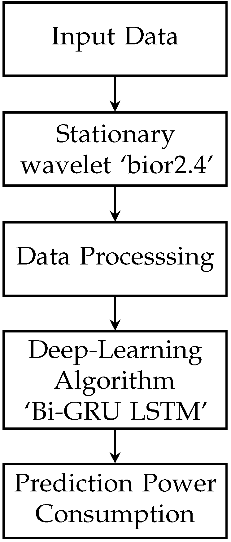
This research establishes a framework for predicting power usage to yield reliable findings. The methodology of this work is presented in Figure 1. This flowchart illustrates the sequence of steps in the proposed algorithm, spanning from data input to model evaluation. Each step is vital for ensuring that the data are correctly processed, the model is accurately trained, and the performance is comprehensively evaluated.

The algorithm begins with the input data stage, where the dataset is collected and loaded. This initial step is crucial to ensure that the data are ready for subsequent processing. Following this, the stationary wavelet transform normalized stage involves applying a stationary wavelet transform (SWT) to the data, followed by normalization. This transformation is essential for converting the data into a form that can be effectively utilized in further processing and modeling.

Next, in the preprocessing data stage, the data undergo various cleaning and preparation procedures. This includes handling missing values, removing noise, and splitting the data into training and testing sets. Additionally, feature engineering may be conducted to enhance the dataset’s utility for the model. This preprocessing step ensures the data are in optimal condition for model training.

The fourth step, training data with the GRU–bior2.4 algorithm, involves initializing the GRU–bior2.4 model and training it using the preprocessed training data. This stage is critical, as it constitutes the core machine learning process where the model learns from the data. The final stage, evaluation model with metric data, focuses on assessing the trained model’s performance using the testing data. Evaluation metrics such as RMSE, MAE, and MAPE are calculated to gauge the model’s performances.

The process concludes with the end stage, marking the completion of the algorithm’s execution. This structured sequence ensures a systematic approach to data handling, model training, and performance evaluation, ultimately leading to a robust and reliable deep learning learning model.

The IHEPC dataset, which is accessible in the UCI repository [48], is used for evaluating the validation of model performance. IHEPC is a free residential dataset obtainable from the machine learning database at UCI that includes electrical consumption data from 2006 to 2010. It has 2,075,259 values, with a total of 25,979 outstanding values. Values that are missing represent 1.25% of the total data and are dealt with at the phase of preprocessing. This dataset contains power usage information at a one-minute sampling rate for over four years. For our evaluation, we separated the data into a set for training and a set for testing. During training, the predictive model is tuned using a training set, and the forecast component predicts values for output from information that are not observed in the testing set. Figure 2 presents the original load profile.

Reliable power consumption forecasts improve energy utilization costs, help organizations make better energy planning choices, and save a significant amount of money and energy. However, forecasting power usage accurately is difficult since it involves dataset dynamics and random fluctuations. In this strategy, 80% of the collected information is utilized for training, while the remaining 20% is used for testing. In a machine learning context, the key objective for our models is to identify the function that relates inputs to outputs using examples from designated training information consisting of known input and output pairs. In order to be processed by our algorithms for forecasting the use of electricity, information should be transformed into an appropriately supervised machine learning issue [38]. As a result, the time series is transformed into pairs of inputs and outputs using the window sliding approach, with 15 past time steps utilized as features to forecast the next step in the time series. The input data are preprocessed in the first stage to eliminate anomalies, missing, and duplicate values. For normalizing the input dataset to a given range, we employ typical scalar approaches. After that, the transformed input data are passed to the training process step. The models LSTM, GRU, Bi-GRU, Bi-LSTM, and Bi-GRU LSTM are then evaluated. Finally, we assess our models using metrics such as RMSE, MAE and MAPE. In simple terms, these measures compute the difference between the expected and real values.

$$RMSE=\sqrt{\left({\displaystyle \frac{{\sum }_{n=1}^N{(y_i-{\widehat{y}}_i)}^2}{N}}\right)}$$

(15)

$$MAE={\displaystyle \frac{{\sum }_{i=0}^{N-1}|y_i-{\widehat{y}}_i|}{N}}$$

(16)

$$MAPE={\displaystyle \frac{100\%}{N}}\sum _{i=0}^{N-1}{\displaystyle \frac{y_i-{\widehat{y}}_i}{y_i}}$$

(17)

where $y_i$, ${\widehat{y}}_i$, and N represent the real value of data, the predicted value of data, and the number of samples of data, respectively.

The Mean Absolute Error (MAE) is a metric that measures the average magnitude of errors in a set of predictions, without considering whether the errors are positive or negative. It is calculated as the mean of the absolute differences between predicted and actual values. In contrast, RMSE assesses the relative difference between predicted and actual values. Meanwhile, MAPE calculates the average absolute percentage error between the forecasted and true values. It offers a clear indication of prediction accuracy in percentage terms, with a lower MAPE signifying better model performance. We also perform experiments on multiple deep learning models for comparison, including LSTM, GRU, Bi-GRU, Bi-LSTM, and Bi-GRU LSTM. The forecasting models are trained for up to 15 epochs using the previously mentioned methodologies. The model is developed using an HP Omen PC equipped with a Core i5 CPU and 16 GB of RAM. The code is written in Python3 Keras, with TensorFlow as the backend and the optimization algorithm Adam.

Table 1. Performance of deep learning models 1 min time stamp.

Deep Learning	RMSE (KWh)	MAE (KWh)	MAPE (%)
LSTM	0.21	0.07	8.55
GRU	0.20	0.07	9.60
Bi-GRU	0.21	0.08	9.94
Bi-LSTM	0.21	0.08	9.15
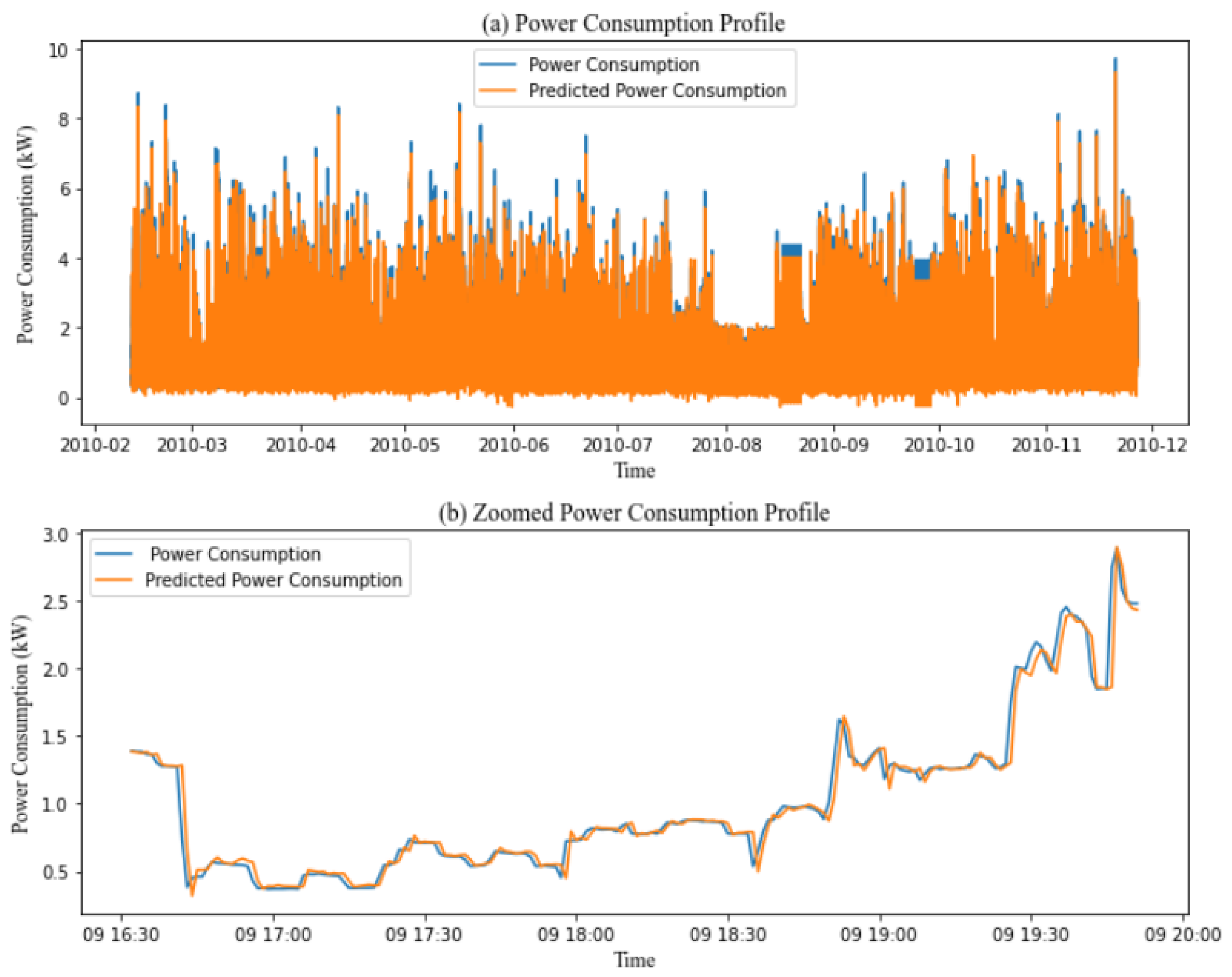
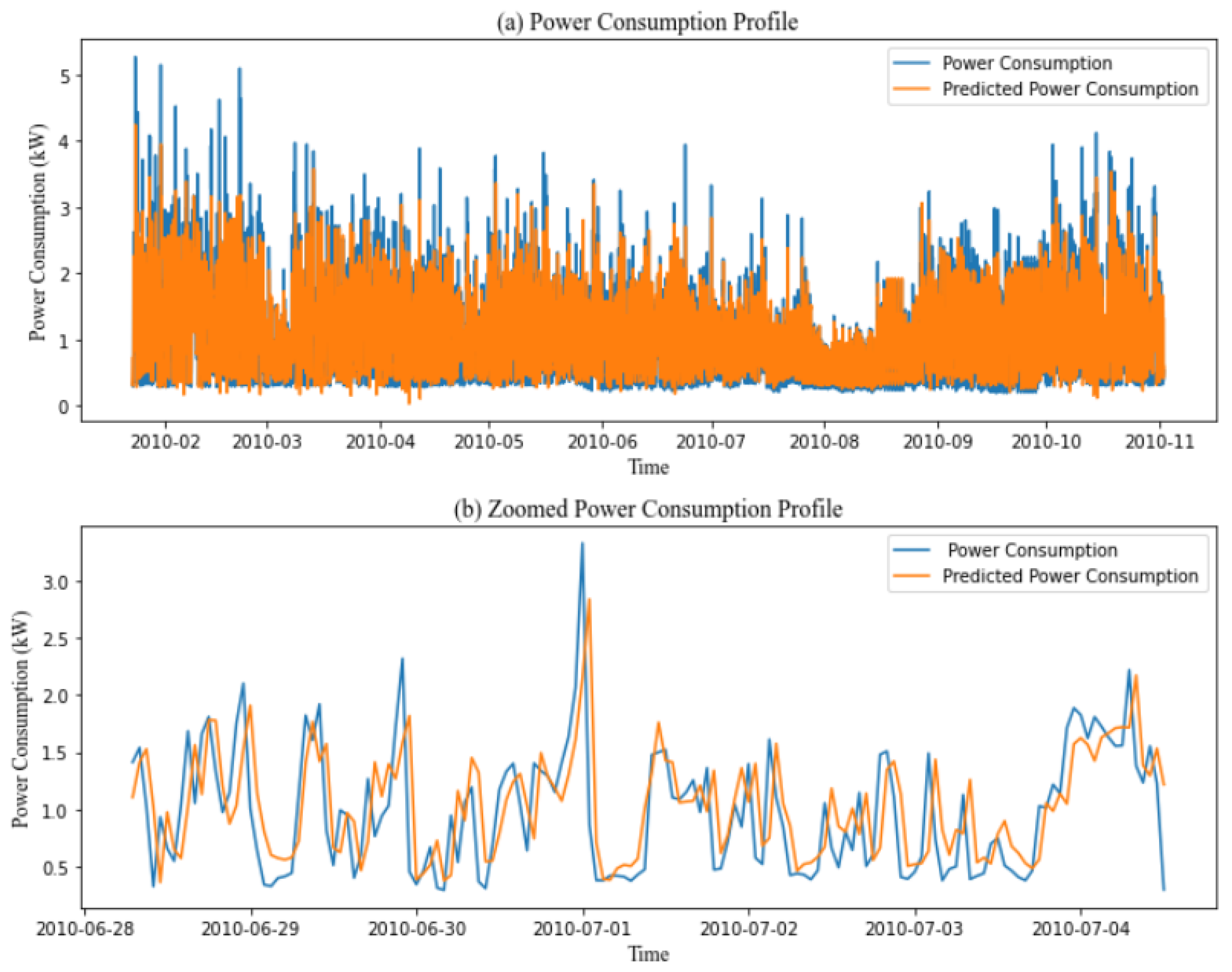
Bi-GRU LSTM	0.21	0.08	8.98

summarizes the results of several deep learning algorithms. LSTM obtained 0.21, 0.07, and 8.55 RMSE, MAE, and MPAE, GRU obtained 0.20, 0.07, and 9.60 RMSE, MAE, and MPAE, Bi-GRU obtained 0.21, 0.08, and 9.94 RMSE, MAE, and MPAE, Bi-LSTM obtained 0.21, 0.08, and 9.15 RMSE, MAE, and MPAE, and Bi-GRU LSTM obtained 0.21, 0.08, and 8.98 RMSE, MAE, and MPAE. Figure 3 illustrates the prediction performance of the GRU model with 1-minute time stamps over the IHEPC dataset and a zoomed-in view of the GRU model’s prediction performance for 1 randomly selected day from the same dataset. Although the predictions in certain areas of Figure 3b appear acceptable, the model’s accuracy could be improved by referring to the MAPE values in the last column of Table 1.

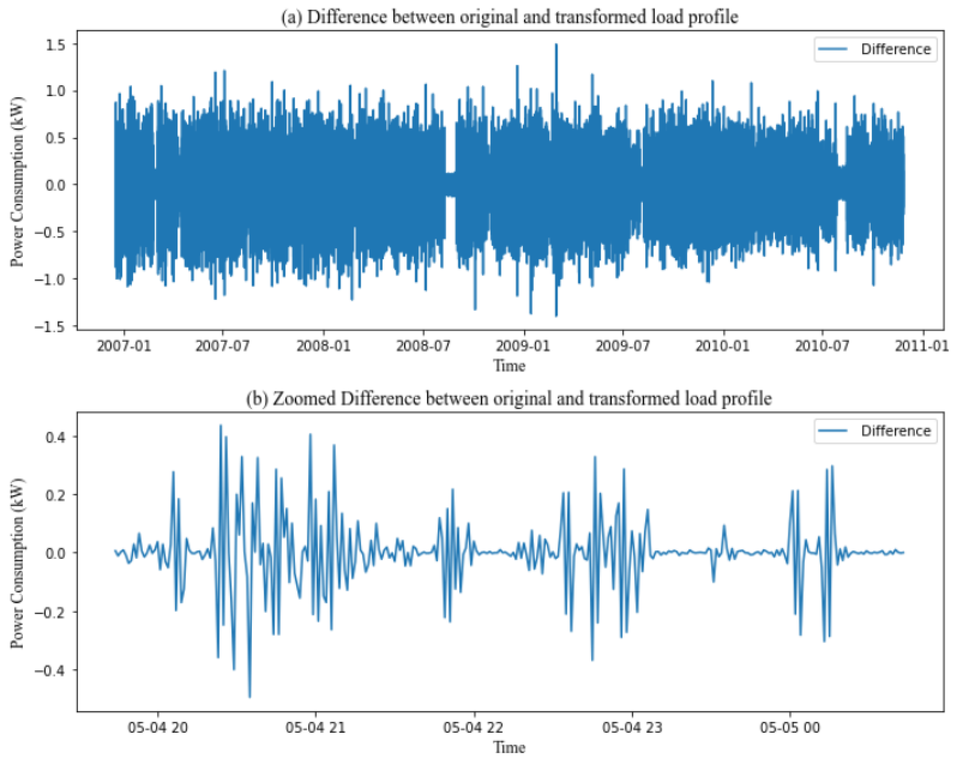
SWT decomposes a signal into high- and low-frequency aspects identified as detail and approximation parameters by feeding it across high-pass and low-pass filters, respectively. The fundamental benefit of SWT is that it overcomes the translation invariance of DWT by eliminating downsamplers and upsamplers. As a result, the SWT variables have the same sampling count as the initial signal. Before proceeding with standard SWT analysis, the following variables must be determined: the mother wavelet and the number of decomposition stages. The mother wavelet is often chosen based on correlations between the mother wavelet and the requested signal. The modified signal has the same shape as the original load profile but with certain modifications. By removing extraneous noise, SWT allows the model to concentrate on the key patterns and relationships within the data. Consequently, we apply a wavelet transform to denoise the original series before modeling. Specifically, the bior2.4 wavelet filter is utilized for stationary wavelet transformation, decomposing each series prior to feeding it into the LSTM, GRU, Bi-LSTM, Bi-GRU, and Bi-GRU LSTM models. Figure 4 shows the difference between the original and transformed load profiles and provides a zoomed-in view of this difference for 1 day.

In the next step, we need to choose the best mother wavelet. So, we introduce a comparative study between different mother wavelets used in the literature. The most popular wavelet are bior2.4, rbio2.4, coif2, db2, and sym2. The competition data exhibit a wide variation in the range of values across different features, which impacts both the accuracy and stability of our forecasting model. To address this, all feature ranges are normalized by rescaling them to a consistent scale. This normalization is performed in Python (version 3.8, developed by the Python Software Foundation, Wilmington, DE, USA) using the MinMaxScaler method from the sklearn package.

Table 2. Accuracy measures of different mother wavelet on SWT using Bi-GRU LSTM 1 min time stamp over IHEPC dataset.

Wavelet + Deep Learning	RMSE (KWh)	MAE (KWh)	MAPE (%)
bior2.4/Bi-GRU LSTM	0.07	0.03	5.09
rbio2.4/Bi-GRU LSTM	0.09	0.06	13.41
db2/Bi-GRU LSTM	0.12	0.05	7.10
coif2/Bi-GRU LSTM	0.23	0.1	12.92
sym2/Bi-GRU LSTM	0.13	0.07	12.81

,

Table 3. Accuracy measures of different mother wavelet on SWT using Bi-GRU 1 min time stamp over IHEPC dataset.

Wavelet + Deep Learning	RMSE (KWh)	MAE (KWh)	MAPE (%)
bior2.4/Bi-GRU	0.07	0.03	5.18
rbio2.4/Bi-GRU	0.07	0.03	6.13
db2/Bi-GRU	0.12	0.05	7.35
coif2/Bi-GRU	0.22	0.08	10.13
sym2/Bi-GRU	0.12	0.06	8.73

,

Table 4. Accuracy measures of different mother wavelet on SWT using Bi-LSTM 1 min time stamp over IHEPC dataset.

Wavelet + Deep Learning	RMSE (KWh)	MAE (KWh)	MAPE (%)
bior2.4/Bi-LSTM	0.07	0.04	7.93
rbio2.4/Bi-LSTM	0.06	0.03	4.92
db2/Bi-LSTM	0.12	0.05	6.49
coif2/Bi-LSTM	0.22	0.08	10.81
sym2/Bi-LSTM	0.12	0.05	7.25

,

Table 5. Accuracy measures of different mother wavelet on SWT using LSTM 1 min time stamp over IHEPC dataset.

Wavelet + Deep Learning	RMSE (KWh)	MAE (KWh)	MAPE (%)
bior2.4/ LSTM	0.07	0.05	8.83
rbio2.4/ LSTM	0.07	0.04	6.53
db2/ LSTM	0.12	0.06	8.13
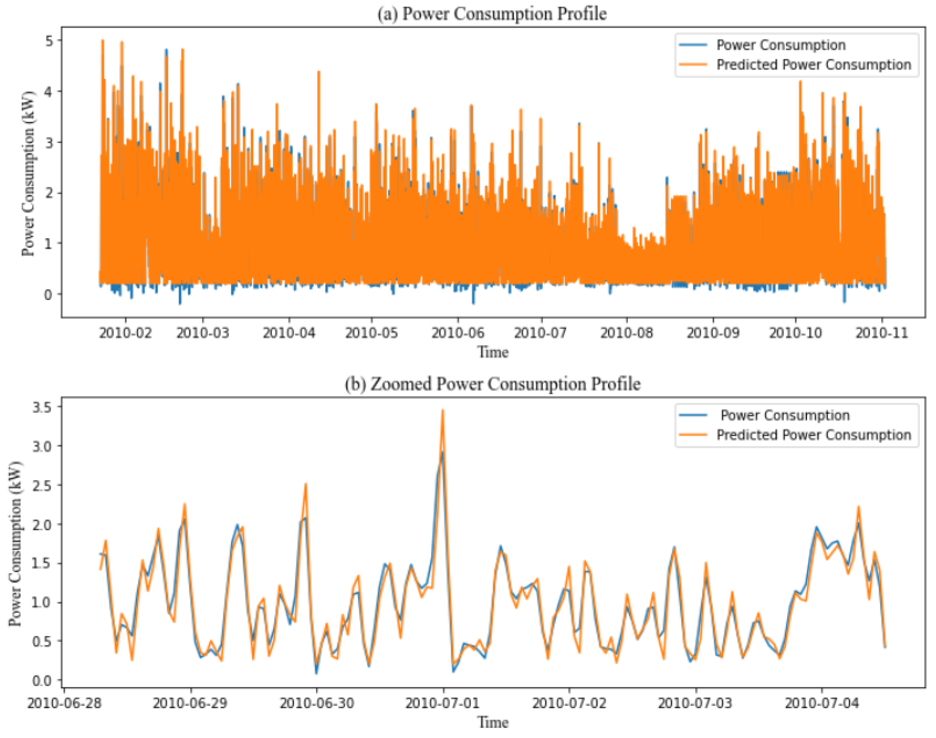
coif2/ LSTM	0.22	0.08	10.76
sym2/ LSTM	0.12	0.05	7.70

and

Table 6. Accuracy measures of different mother wavelet on SWT using GRU 1 min time stamp over IHEPC dataset.

Wavelet + Deep Learning	RMSE (KWh)	MAE (KWh)	MAPE (%)
bior2.4/GRU	0.06	0.03	5.65
rbio2.4/GRU	0.07	0.04	7.76
db2/GRU	0.12	0.05	7.14
coif2/GRU	0.22	0.10	14.25
sym2/GRU	0.12	0.05	7.15

summarize the findings of several mother wavelets bior2.4, rbio2.4, coif2, db2, and sym2 with different deep learning algorithms LSTM, GRU, Bi-LSTM, Bi-GRU, and Bi-GRU LSTM. The results found show that bior2.4 is the most relevant mother wavelet compared to the mother wavelets used for all deep learning models. For bior2.4 with deep learning models, we see significant improvement in energy consumption prediction accuracy. bior2.4/LSTM obtained 0.07, 0.03, and 8.83 RMSE, MAE, and MPAE. These results show improvements in RMSE and MAE by 66.66% and 28% respectively. bior2.4/GRU obtained 0.06, 0.04, and 5.65. These results demonstrate improvements in RMSE, MAE, and MPAE by 70%, 42.85%, and 47.67%, respectively. bior2.4/Bi-LSTM achieved RMSE, MAE, and MPAE scores of 0.07, 0.04, and 7.93 respectively. These results represent improvements of 66.66%, 42.85%, and 7.25% in RMSE, MAE, and MPAE. bior2.4/Bi-GRU achieved scores of 0.07, 0.03, and 5.18, respectively, demonstrating improvements of 66.66%, 62.5%, and 46.04% in RMSE, MAE, and MPAE. Bi-GRU LSTM obtained 0.07, 0.03, and 5.09 RMSE, MAE, and MPAE. These results represent improvements of 66.66%, 42.85%, and 43.31% in RMSE, MAE, and MPAE. Based on these results, we can conclude that the bior2.4/GRU model provides the most accurate predictions. So we accurately predict the challenging numbers associated with significant variance in power consumption, resulting in precise and reliable power usage forecasts as shown in Figure 5 which illustrates the prediction performance of the proposed model with 1-minute time stamps over the IHEPC dataset and a zoomed-in view of the proposed model’s prediction performance for 1 randomly selected day from the same dataset.

Table 7. Performance of deep learning model 15 min time stamp.

Deep Learning	RMSE (KWh)	MAE (KWh)	MAPE (%)
LSTM	0.47	0.28	38.41
GRU	0.46	0.28	39.13
Bi-GRU	0.46	0.28	43.58
Bi-LSTM	0.46	0.28	37.75
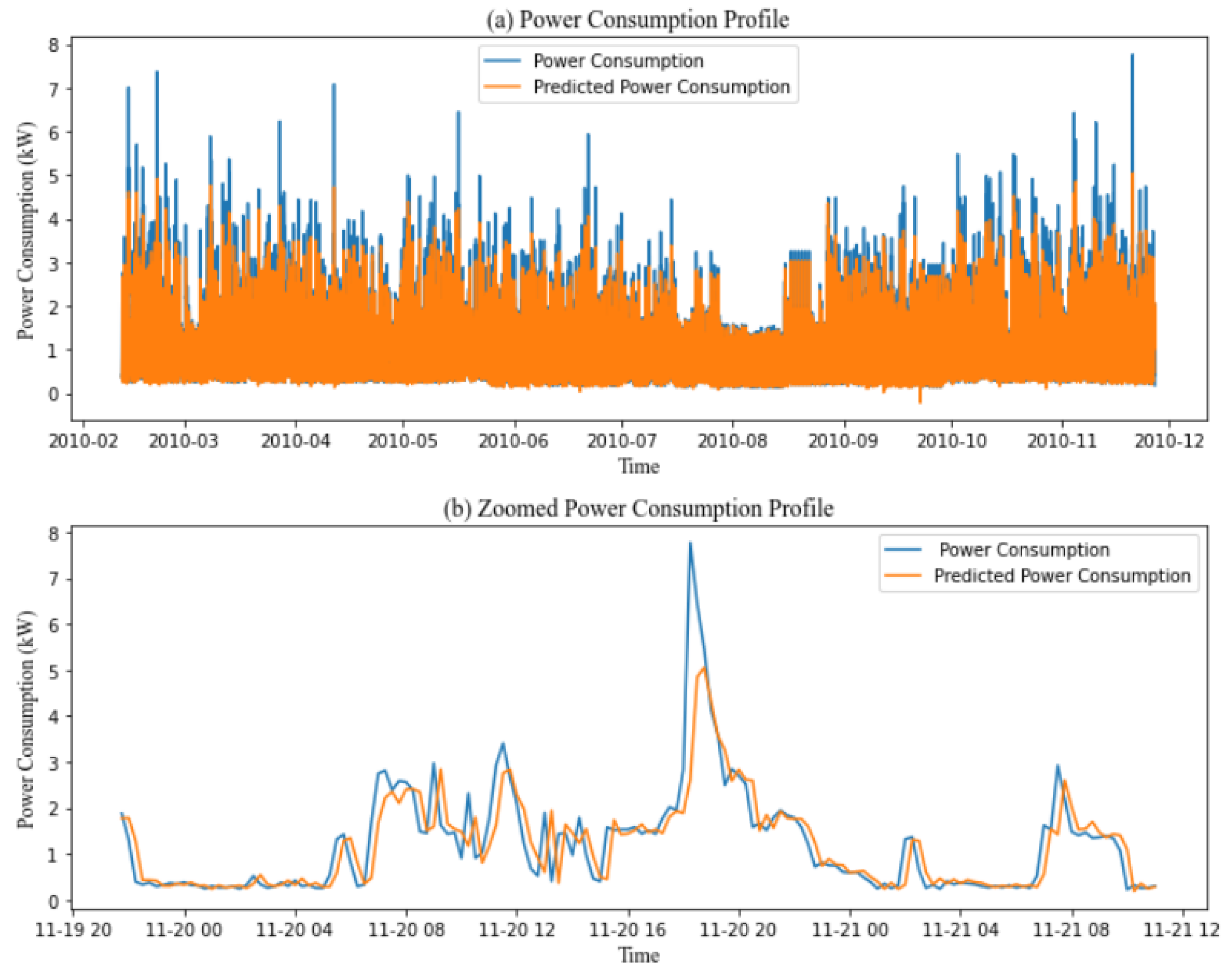
Bi-GRU LSTM	0.47	0.29	40.75

summarizes the results of several deep learning algorithms. LSTM obtained 0.46, 0.28 and 38.41 RMSE, MAE and MPAE; GRU obtained 0.46, 0.28 and 39.13 RMSE, MAE and MPAE; Bi-GRU obtained 0.46, 0.28, and 43.58 RMSE, MAE, and MPAE; Bi-LSTM obtained 0.46, 0.28, and 37.75 RMSE, MAE and MPAE; and Bi-GRU LSTM obtained 0.47, 0.29, and 40.75 RMSE, MAE and MPAE. The model fails to estimate the precise value when there is a quick change or a peak in consumption. The results suggest that employing deep learning algorithms to estimate power usage is not always reliable as shown in Figure 6. Several factors influence the prediction performance, such as lowering the quantity of data in the database utilized by the model.

Table 8. Accuracy measures of bior2.4 mother wavelet on SWT using deep learning algorithms 15 min time stamp over the IHEPC dataset.

Wavelet + Deep Learning	RMSE (KWh)	MAE (KWh)	MAPE (%)
bior2.4/Bi-GRU LSTM	0.16	0.11	15.66
bior2.4/Bi-GRU	0.15	0.10	15.07
bior2.4/Bi-LSTM	0.15	0.11	17.55
bior2.4/LSTM	0.15	0.10	13.55
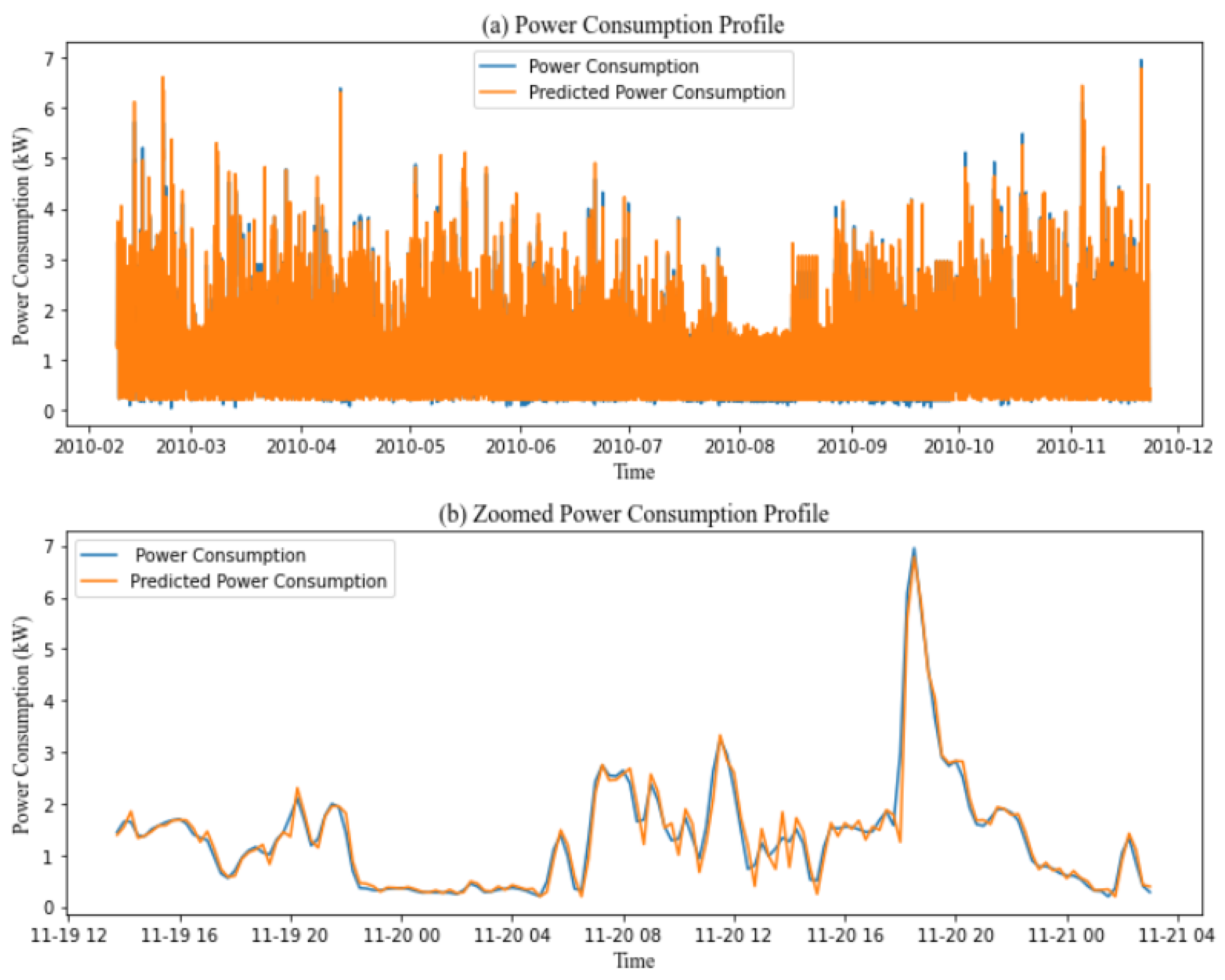
bior2.4/GRU	0.15	0.1	13.62

summarizes the findings for mother wavelet bior2.4 combined with different deep learning algorithms (LSTM, GRU, Bi-LSTM, Bi-GRU, and Bi-GRU LSTM). For bior2.4 paired with these models, there is a notable improvement in the energy consumption prediction accuracy. bior2.4/LSTM achieved RMSE, MAE, and MPAE scores of 0.16, 0.11, and 15.66, respectively, showing improvements of 65.95%, 60.71%, and 59.22% in RMSE, MAE, and MAPE. bior2.4/GRU obtained scores of 0.15, 0.10, and 13.62, demonstrating improvements of 67.73%, 64.28%, and 65.19% in RMSE, MAE, and MPAE. bior2.4/Bi-LSTM recorded RMSE, MAE, and MPAE scores of 0.15, 0.11, and 17.55, reflecting improvements of 67.39%, 60.71%, and 53.50%. bior2.4/Bi-GRU achieved 0.15, 0.10, and 15.07 in RMSE, MAE, and MPAE, showing improvements of 67.39%, 64.28%, and 59.72%. bior2.4/Bi-GRU LSTM obtained scores of 0.16, 0.11, and 15.66, with improvements of 65.95%, 62.06%, and 61.57%. From these results obtained, we can deduce that the bior2.4/GRU model gives the most precise model. These findings confirm our ability to accurately predict the challenging numbers associated with significant variance in power consumption, resulting in precise and reliable power usage forecasts as shown in Figure 7.

Table 9. Performance of deep learning models with a 1 h time stamp.

Deep Learning	RMSE (KWh)	MAE (KWh)	MAPE (%)
LSTM	0.52	0.37	52.39
GRU	0.52	0.38	55.44
Bi-GRU	0.52	0.36	47.28
Bi-LSTM	0.51	0.36	49.71
Bi-GRU LSTM	0.52	0.37	52.72

summarizes the results of several deep learning algorithms. LSTM obtained 0.50, 0.37, and 52.39 RMSE, MAE, and MPAE; GRU obtained 0.52, 0.38, and 55.44 RMSE, MAE, and MPAE; Bi-GRU obtained 0.52, 0.36, and 47.28 RMSE, MAE, and MPAE; Bi-LSTM obtained 0.51, 0.36, and 49.71 RMSE, MAE and MPAE; and Bi-GRU LSTM obtained 0.52, 0.37, and 52.72 RMSE, MAE, and MPAE. The model struggles to accurately estimate values during sudden changes or peaks in consumption. The findings indicate that using deep learning algorithms to predict power usage can sometimes be unreliable. Various factors, including a reduction in the amount of data available to the model, affect its prediction performance as demonstrated in Figure 8.

Table 10. Accuracy measures of bior2.4 mother wavelet on SWT using deep learning algorithms with a 1 h time stamp over the IHEPC dataset.

Wavelet + Deep Learning	RMSE (KWh)	MAE (KWh)	MAPE (%)
bior2.4/Bi-GRU LSTM	0.18	0.13	17.91
bior2.4/Bi-GRU	0.17	0.13	17.53
bior2.4/Bi-LSTM	0.18	0.14	20.83
bior2.4/LSTM	0.18	0.13	18.98
bior2.4/GRU	0.18	0.13	18.21

summarizes the results for mother wavelet bior2.4 combined with different deep learning algorithms (LSTM, GRU, Bi-LSTM, Bi-GRU, and Bi-GRU LSTM). Pairing bior2.4 with these models leads to significant improvements in predicting energy consumption accuracy. bior2.4/LSTM achieved RMSE, MAE, and MPAE scores of 0.18, 0.13, and 18.98, respectively, showing improvements of 65.38%, 64.48%, and 63.77% in RMSE, MAE, and MAPE. bior2.4/GRU obtained scores of 0.18, 0.13, and 18.21, demonstrating improvements of 65.38%, 65.78%, and 67.15% in RMSE, MAE, and MPAE. bior2.4/Bi-LSTM recorded RMSE, MAE, and MPAE scores of 0.18, 0.14, and 20.83, reflecting improvements of 64.70%, 61.11%, and 58.09%. bior2.4/Bi-GRU achieved scores of 0.17, 0.13, and 17.53 in RMSE, MAE, and MPAE, showing improvements of 67.30%, 63.88%, and 62.92%. bior2.4/Bi-GRU LSTM obtained scores of 0.18, 0.13, and 17.91, reflecting improvements of 65.38%, 64.86%, and 66.02%. These results indicate that the bior2.4/Bi-GRU and bior2.4/GRU models give the most accurate predictions. The results of these two models are nearly identical across all metrics used to assess accuracy. However, since the simulation time of the bior2.4/GRU model is faster than that of the bior2.4/Bi-GRU model, we can conclude that the bior2.4/GRU model is more efficient for predicting power consumption. These results validate our capability to precisely forecast the demanding figures linked with notable fluctuations in power consumption, leading to dependable and accurate predictions of power usage as shown in Figure 9.

Our analysis shows that the proposed model excels in predicting sudden changes or peaks in consumption more accurately than deep learning algorithms. Although wavelet and deep learning methods are generally dependable for forecasting power consumption, the proposed model surpasses these approaches in both precision and reliability. Several factors affect the performance of the prediction such as reducing the amount of data and complexity in the database used in the model. These methods have been demonstrated to generate reliable forecasts. While various methods exist for predicting power consumption, they often fail to consistently achieve expected performance levels due to their unique advantages and disadvantages. Denoising helps remove unnecessary noise, enabling the model to focus on the essential patterns and correlations within the data. As a result, the original time series was denoised using wavelet transformation prior to applying the model. The stationary wavelet transform was performed using the bior2.4 wavelet filter, decomposing each series before feeding it into the LSTM, GRU, Bi-LSTM, Bi-GRU, and Bi-GRU LSTM models. The models’ hyperparameters were fine-tuned through numerous simulations of expected values. In this database, we employed many domestic devices such as a dishwasher, an oven, and a microwave in the kitchen. In the laundry area, we also have a washing machine, a tumble dryer, a refrigerator, and a lamp. We utilized a water heater that was powered by electricity and an air conditioner in the remainder of the residence. It is critical to reduce the prediction error associated with sudden fluctuations. Our model is able to predict the sudden change in electric charge when using critical loads like washing machines, ovens, and air conditioners.

5. Conclusions

Building safe, dependable, entirely automated smart grid systems necessitates the use of a reliable power consumption modeling system. This work makes two significant contributions to the field of energy forecasting, showcasing advancements in both analytical methods and predictive modeling.

Firstly, the application of biorthogonal wavelets (bior2.4) for time series decomposition represents a major innovation. Its properties of perfect reconstruction and symmetry have proven highly effective in analyzing energy consumption patterns. By employing the stationary wavelet transform (SWT), we extracted detailed insights from various frequency components of the time series data. This method offers a more refined understanding of short-term fluctuations and long-term trends in energy consumption.

Secondly, the incorporation of Gated Recurrent Units (GRUs) into predictive models marks a notable advancement in deep learning. GRUs, with their sophisticated architecture, excel at processing sequential data and capturing time-dependent patterns, making them particularly reliable for energy forecasting. The synergy between GRU modeling and stationary wavelet-transformed data with mother wavelet bior2.4 significantly enhanced prediction accuracy. The models were rigorously validated using a real-world electrical load forecasting dataset on different time stamps 1 min, 15 min, and 1 h. It is important to note whether or not the choice of intervals 1 min, 15 min, and 1 h affects the accuracy and reliability of the proposed method. Based on the analysis, the difference between these intervals significantly impacts the predictive performance. For example, the prediction accuracy decreases as the interval duration increases as shown by quantitative error measurements such as the Mean Absolute Error (MAE) and Root Mean Square Error (RMSE). This indicates that shorter intervals result in more accurate predictions, thus demonstrating the sensitivity of the method to interval length. Comparative analysis between SWT with the bior2.4 filter and traditional models confirmed the substantial improvement in predictive accuracy introduced by wavelet transforms. Across all time intervals, denoising consistently led to significant reductions in error metrics, with decreases ranging from 60% to over 70%. These findings emphasize the potential of integrating advanced analytical techniques with innovative deep learning methods to improve forecasting accuracy and reliability, contributing valuable insights to the field and setting the stage for future research and practical applications.

References

1. Sajjad, M.; Khan, Z.A.; Ullah, A.; Hussain, T.; Ullah, W.; Lee, M.Y.; Baik, S.W. A novel CNN-GRU-based hybrid approach for short-term residential load forecasting. IEEE Access 2020, 8, 143759–143768. [Google Scholar] [CrossRef]
2. World Energy Outlook 2019. 2019. Available online: https://www.iea.org/reports/world-energy-outlook-2019 (accessed on 12 November 2023).
3. Nejat, P.; Jomehzadeh, F.; Taheri, M.M.; Gohari, M.; Majid, M.Z.A. A global review of energy consumption CO2 emissions and policy in the residential sector (with an overview of the top ten CO2 emitting countries). Renew. Sustain. Energy Rev. 2015, 43, 843–862. [Google Scholar] [CrossRef]
4. Kim, T.Y.; Cho, S.B. Predicting residential energy consumption using CNN-LSTM neural networks. Energy 2019, 182, 72–81. [Google Scholar] [CrossRef]
5. Tran, V.G.; Debusschere, V.; Bacha, S. One week hourly electricity load forecasting using neuro-fuzzy and seasonal ARIMA models. IFAC Proc. Vol. 2012, 45, 97–102. [Google Scholar] [CrossRef]
6. Deb, C.; Zhang, F.; Yang, J.; Lee, S.E.; Shah, K.W. A review on time series forecasting techniques for building energy consumption. Renew. Sustain. Energy Rev. 2017, 74, 902–924. [Google Scholar] [CrossRef]
7. Ahmad, M.I. Seasonal decomposition of electricity consumption data. Rev. Integr. Bus. Econ. Res. 2017, 6, 271–275. [Google Scholar]
8. Chou, J.S.; Tran, D.S. Forecasting energy consumption time series using machine learning techniques based on usage patterns of residential householders. Energy 2018, 165, 709–726. [Google Scholar] [CrossRef]
9. Wei, N.; Li, C.; Peng, X.; Zeng, F.; Lu, X. Conventional models and artificial intelligence-based models for energy consumption forecasting: A review. J. Pet. Sci. Eng. 2019, 181, 106187. [Google Scholar] [CrossRef]
10. de Oliveira, E.M.; Oliveira, F.L.C. Forecasting mid-long term electric energy consumption through bagging ARIMA and exponential smoothing methods. Energy 2018, 144, 776–788. [Google Scholar] [CrossRef]
11. Fumo, N.; Biswas, M.A.R. Regression analysis for prediction of residential energy consumption. Renew. Sustain. Energy Rev. 2015, 47, 332–343. [Google Scholar] [CrossRef]
12. Amber, K.P.; Aslam, M.W.; Hussain, S.K. Electricity consumption forecasting models for administration buildings of the UK higher education sector. Energy Build. 2015, 90, 127–136. [Google Scholar] [CrossRef]
13. Jain, R.K.; Smith, K.M.; Culligan, P.J.; Taylor, J.E. Forecasting energy consumption of multi-family residential buildings using support vector regression: Investigating the impact of temporal and spatial monitoring granularity on performance accuracy. Appl. Energy 2014, 123, 168–178. [Google Scholar] [CrossRef]
14. Yaslan, Y.; Bican, B. Empirical mode decomposition based denoising method with support vector regression for time series prediction: A case study for electricity load forecasting. Measurement 2017, 103, 52–61. [Google Scholar] [CrossRef]
15. Rueda, R.; Cuéllar, M.P.; Pegalajar, M.C.; Delgado, M. Straight line programs for energy consumption modelling. Appl. Soft Comput. 2019, 80, 310–328. [Google Scholar] [CrossRef]
16. Liu, Y.; Chen, H.; Zhang, L.; Wu, X.; Wang, X.J. Energy consumption prediction and diagnosis of public buildings based on support vector machine learning: A case study in China. J. Clean. Prod. 2020, 272, 122542. [Google Scholar] [CrossRef]
17. Chen, Y.; Xu, P.; Chu, Y.; Li, W.; Wu, Y.; Ni, L.; Bao, Y.; Wang, K. Short-term electrical load forecasting using the support vector regression (SVR) model to calculate the demand response baseline for office buildings. Appl. Energy 2017, 195, 659–670. [Google Scholar] [CrossRef]
18. Bogomolov, A.; Lepri, B.; Larcher, R.; Antonelli, F.; Pianesi, F.; Pentland, A. Energy consumption prediction using people dynamics derived from cellular network data. EPJ Data Sci. 2016, 5, 1–13. [Google Scholar] [CrossRef]
19. Khan, A.; Chiroma, H.; Imran, M.; Khan, A.; Bangash, J.I.; Asim, M.; Aljuaid, H. Forecasting electricity consumption based on machine learning to improve performance: A case study for the organization of petroleum exporting countries (OPEC). Comput. Electr. Eng. 2020, 86, 106737. [Google Scholar] [CrossRef]
20. Pinto, T.; Praça, I.; Vale, Z.; Silva, J. Ensemble learning for electricity consumption forecasting in office buildings. Neurocomputing 2021, 423, 747–755. [Google Scholar] [CrossRef]
21. Rahman, A.; Srikumar, V.; Smith, A.D. Predicting electricity consumption for commercial and residential buildings using deep recurrent neural networks. Appl. Energy 2018, 212, 372–385. [Google Scholar] [CrossRef]
22. Shi, H.; Xu, M.; Li, R. Deep learning for household load forecasting—A novel pooling deep RNN. IEEE Trans. Smart Grid 2018, 9, 5271–5280. [Google Scholar] [CrossRef]
23. Kong, W.; Dong, Z.Y.; Jia, Y.; Hill, D.J.; Xu, Y.; Zhang, Y. Short-term residential load forecasting based on LSTM recurrent neural network. IEEE Trans. Smart Grid 2019, 10, 841–851. [Google Scholar] [CrossRef]
24. Wang, J.Q.; Du, Y.; Wang, J. LSTM based long-term energy consumption prediction with periodicity. Energy 2020, 197, 117197. [Google Scholar] [CrossRef]
25. Hu, H.; Wang, L.; Peng, L.; Zeng, Y.R. Effective energy consumption forecasting using enhanced bagged echo state network. Energy 2020, 193, 116778. [Google Scholar] [CrossRef]
26. Fayaz, M.; Kim, D. A prediction methodology of energy consumption based on deep extreme learning machine and comparative analysis in residential buildings. Electronics 2018, 7, 222. [Google Scholar] [CrossRef]
27. Gao, Y.; Ruan, Y.; Fang, C.; Yin, S. Deep learning and transfer learning models of energy consumption forecasting for a building with poor information data. Energy Build. 2020, 223, 110156. [Google Scholar] [CrossRef]
28. Frikha, M.; Taouil, K.; Fakhfakh, A.; Derbel, F. Limitation of Deep-Learning Algorithm for Prediction of Power Consumption. Eng. Proc. 2022, 18, 26. [Google Scholar] [CrossRef]
29. Fan, G.F.; Wei, X.; Li, Y.T.; Hong, W.C. Forecasting electricity consumption using a novel hybrid model. Sustain. Cities Soc. 2020, 61, 102320. [Google Scholar] [CrossRef]
30. Xiao, J.; Li, Y.; Xie, L.; Liu, D.; Huang, J. A hybrid model based on selective ensemble for energy consumption forecasting in China. Energy 2018, 159, 534–546. [Google Scholar] [CrossRef]
31. Hu, H.; Wang, L.; Lv, S.X. Forecasting energy consumption and wind power generation using deep echo state network. Renew. Energy 2020, 154, 598–613. [Google Scholar] [CrossRef]
32. Xia, C.; Wang, Z. Drivers analysis and empirical mode decomposition based forecasting of energy consumption structure. J. Clean. Prod. 2020, 254, 120107. [Google Scholar] [CrossRef]
33. Kaytez, F. A hybrid approach based on autoregressive integrated moving average and least-square support vector machine for long-term forecasting of net electricity consumption. Energy 2020, 197, 117200. [Google Scholar] [CrossRef]
34. Liu, T.; Tan, Z.; Xu, C.; Chen, H.; Li, Z. Study on deep reinforcement learning techniques for building energy consumption forecasting. Energy Build. 2020, 208, 109675. [Google Scholar] [CrossRef]
35. Zhang, G.; Tian, C.; Li, C.; Zhang, J.J.; Zuo, W. Accurate forecasting of building energy consumption via a novel ensembled deep learning method considering the cyclic feature. Energy 2020, 201, 117531. [Google Scholar] [CrossRef]
36. Kazemzadeh, M.R.; Amjadian, A.; Amraee, T. A hybrid data mining driven algorithm for long term electric peak load and energy demand forecasting. Energy 2020, 204, 117948. [Google Scholar] [CrossRef]
37. Cheng, M.Y.; Vu, Q.T. Bio-inspired bidirectional deep machine learning for real-time energy consumption forecasting and management. Energy 2024, 302, 131720. [Google Scholar] [CrossRef]
38. Lu, H.; Cheng, F.; Ma, X.; Hu, G. Short-term prediction of building energy consumption employing an improved extreme gradient boosting model: A case study of an intake tower. Energy 2020, 203, 117756. [Google Scholar] [CrossRef]
39. Ullah, F.U.M.; Ullah, A.; Haq, I.U.; Rho, S.; Baik, S.W. Short-term prediction of residential power energy consumption via CNN and multi-layer bi-directional LSTM networks. IEEE Access 2020, 8, 123369–123380. [Google Scholar] [CrossRef]
40. Liu, D.; Wang, H. Time series analysis model for forecasting unsteady electric load in buildings. Energy Built Environ. 2024, 5, 900–910. [Google Scholar] [CrossRef]
41. Yan, K.; Li, W.; Ji, Z.; Qi, M.; Du, Y. A hybrid LSTM neural network for energy consumption forecasting of individual households. IEEE Access 2019, 7, 157633–157642. [Google Scholar] [CrossRef]
42. Singla, P.; Duhan, M.; Saroha, S. An ensemble method to forecast 24-h ahead solar irradiance using wavelet decomposition and BiLSTM deep learning network. Earth Sci. Inform. 2022, 15, 291–306. [Google Scholar] [CrossRef] [PubMed]
43. Lin, Y.; Chen, K.; Zhang, X.; Tan, B.; Lu, Q. Forecasting crude oil futures prices using BiLSTM-Attention-CNN model with Wavelet transform. Appl. Soft Comput. 2022, 130, 109723. [Google Scholar] [CrossRef]
44. Eneyew, D.D.; Capretz, M.A.M.; Bitsuamlak, G.T.; Mir, S. Predicting Residential Energy Consumption Using Wavelet Decomposition With Deep Neural Network. In Proceedings of the 2020 19th IEEE International Conference on Machine Learning and Applications (ICMLA), Miami, FL, USA, 14–17 December 2020; pp. 895–900. [Google Scholar] [CrossRef]
45. Saoud, L.S.; Al-Marzouqi, H.; Hussein, R. Household Energy Consumption Prediction Using the Stationary Wavelet Transform and Transformers. IEEE Access 2022, 10, 5171–5183. [Google Scholar] [CrossRef]
46. Kondaiah, V.Y.; Saravanan, B. Short-Term Load Forecasting with a Novel Wavelet-Based Ensemble Method. Energies 2022, 15, 5299. [Google Scholar] [CrossRef]
47. Tamilselvi, C.; Yeasin, M.; Paul, R.K.; Paul, A.K. Can Denoising Enhance Prediction Accuracy of Learning Models? A Case of Wavelet Decomposition Approach. Forecasting 2024, 6, 81–99. [Google Scholar] [CrossRef]
48. Dua, D.; Graff, C. UCI Machine Learning Repository; University of California, School of Information and Computer Sciences: Irvine, CA, USA, 2019. Available online: http://archive.ics.uci.edu/ml (accessed on 20 January 2022).
Figure 1. Flowchart of the proposed algorithm.
Forecasting 06 00043 g001
Figure 2. Load profile of 1 min time stamp over IHEPC dataset.
Forecasting 06 00043 g002
Figure 3. (a) Prediction performance of the GRU model 1 min time stamp over IHEPC dataset. (b) Zoomed-in part 1 day of prediction performance of GRU model 1 min time stamp over IHEPC dataset.
Forecasting 06 00043 g003
Figure 4. (a) Difference between original and transformed load profile. (b) Zoomed-in part 1 day of the difference between the original and transformed load profile.
Forecasting 06 00043 g004
Figure 5. (a) Prediction performance of the proposed model 1 min time stamp over the IHEPC dataset; (b) zoomed-in part of 1 day of the prediction performance of the proposed model with a 1 min time stamp over the IHEPC dataset.
Forecasting 06 00043 g005
Figure 6. (a) Prediction performance of the GRU model with a 15 min time stamp over the IHEPC dataset. (b) Zoomed-in part of 3 days of the prediction performance of the GRU model with a 15 min time stamp over the IHEPC dataset.
Forecasting 06 00043 g006
Figure 7. (a) Prediction performance of the proposed model with a 15 min time stamp over the IHEPC dataset. (b) Zoomed-in part of 3 days of the prediction performance of the proposed model with a 15 min time stamp over the IHEPC dataset.
Forecasting 06 00043 g007
Figure 8. (a) Prediction performance of the GRU model with a 1 h time stamp over the IHEPC dataset. (b) Zoomed-in part of 6 days of the prediction performance of the GRU model with a 1 h time stamp over the IHEPC dataset.
Forecasting 06 00043 g008
Figure 9. (a) Prediction performance of the proposed model with a 1 h time stamp over the IHEPC dataset. (b) Zoomed-in part of 6 days of the prediction performance of the proposed model with a 1 h time stamp over the IHEPC dataset.
Forecasting 06 00043 g009