
Global Solar Radiation Forecasting Based on Hybrid Model with Combinations of Meteorological Parameters: Morocco Case Study


Abstract
:1. Introduction
2. Materials and Methods
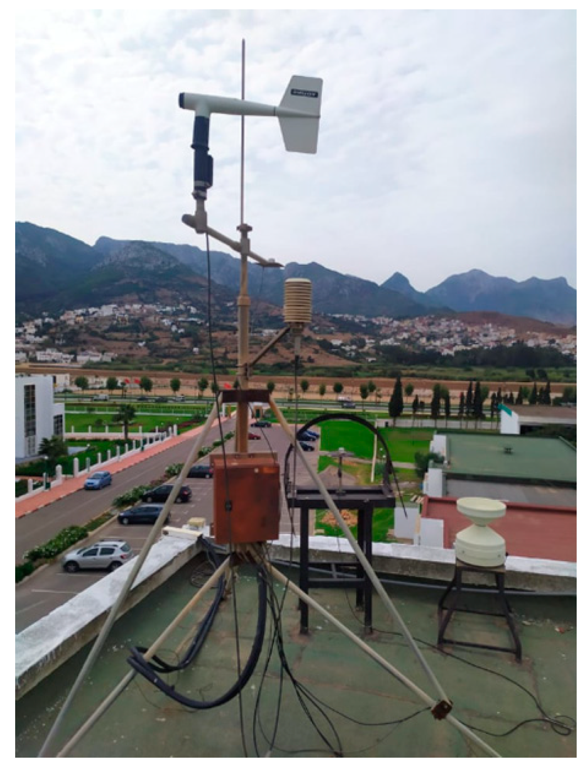
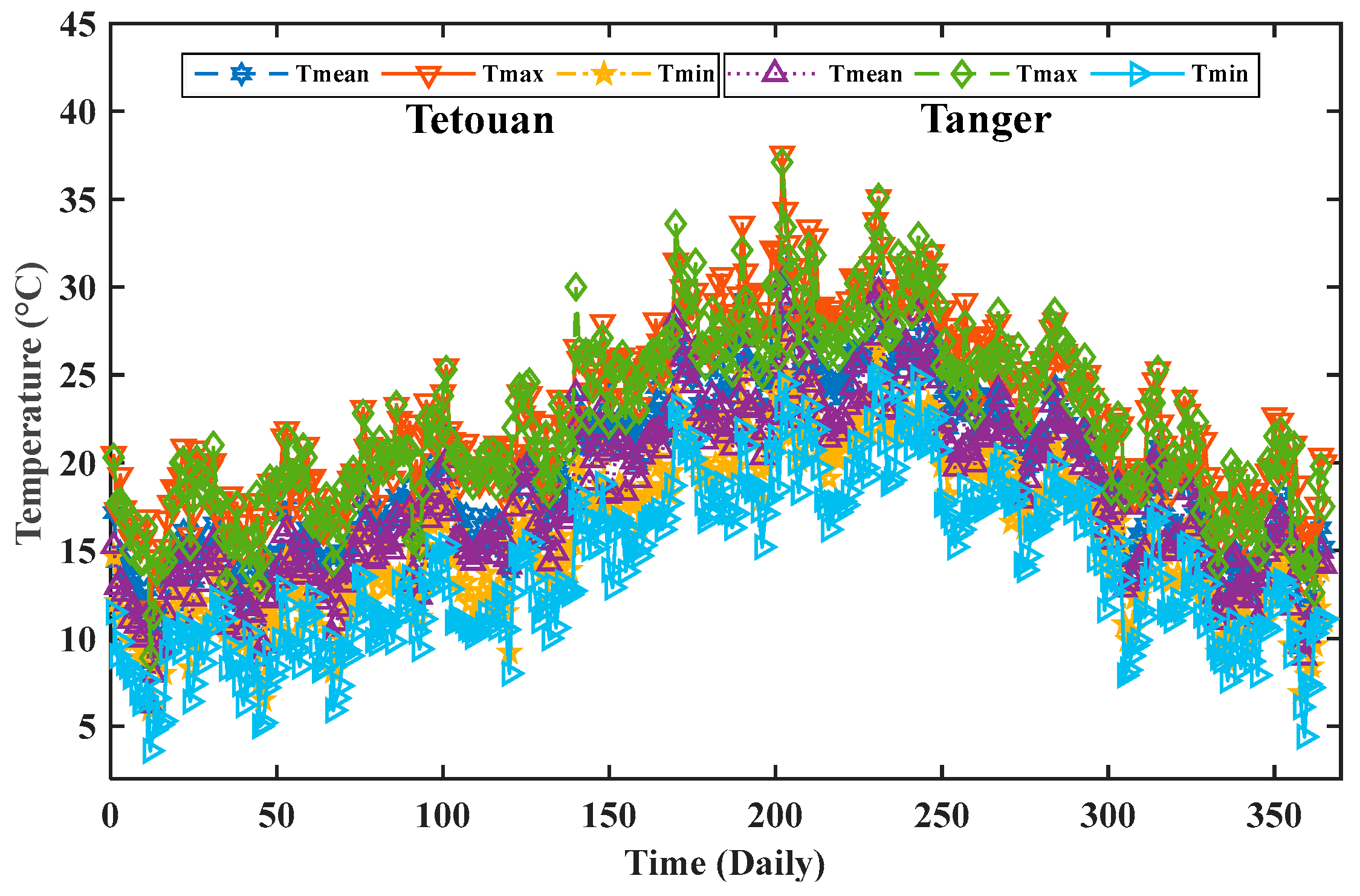
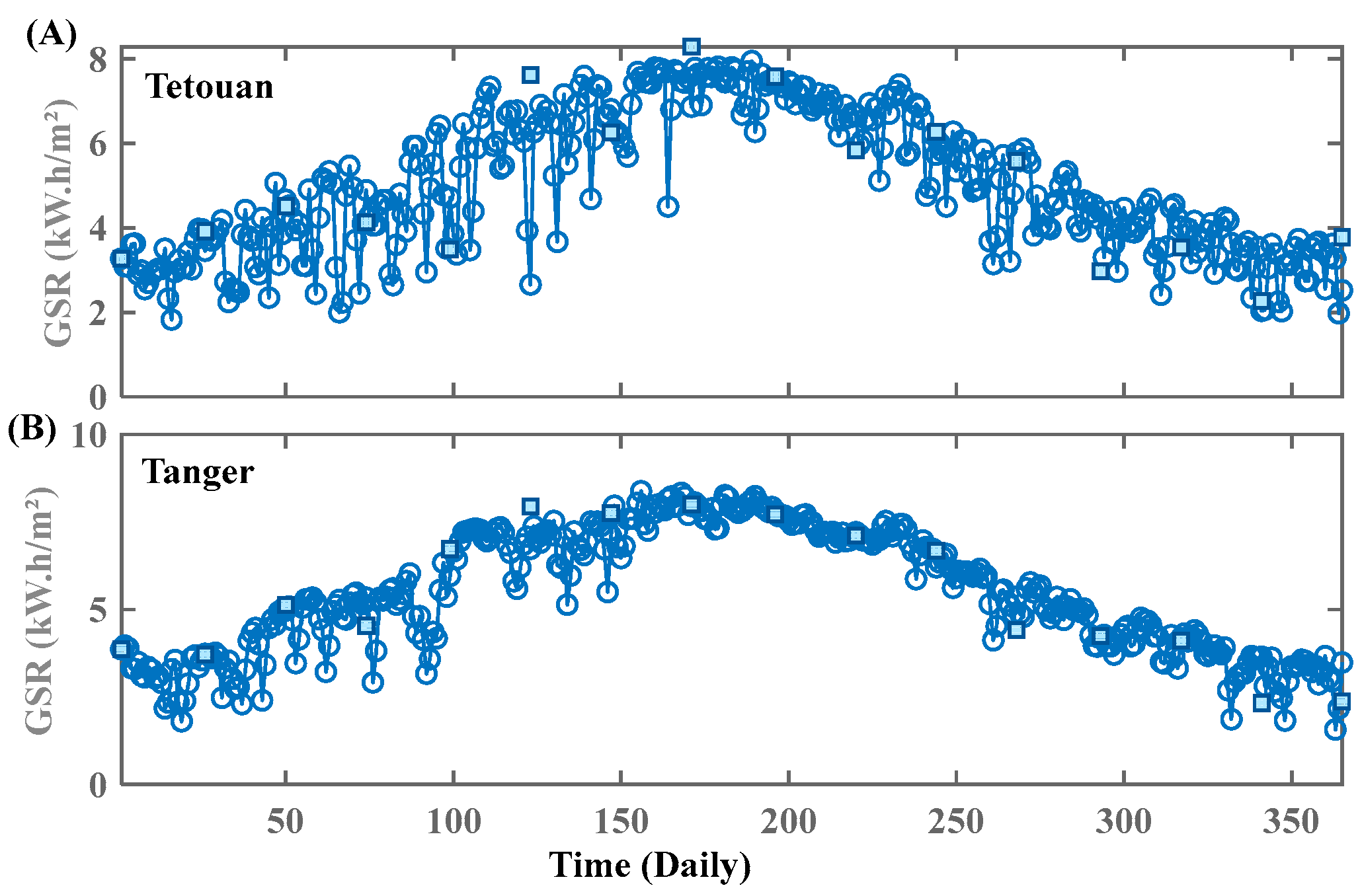
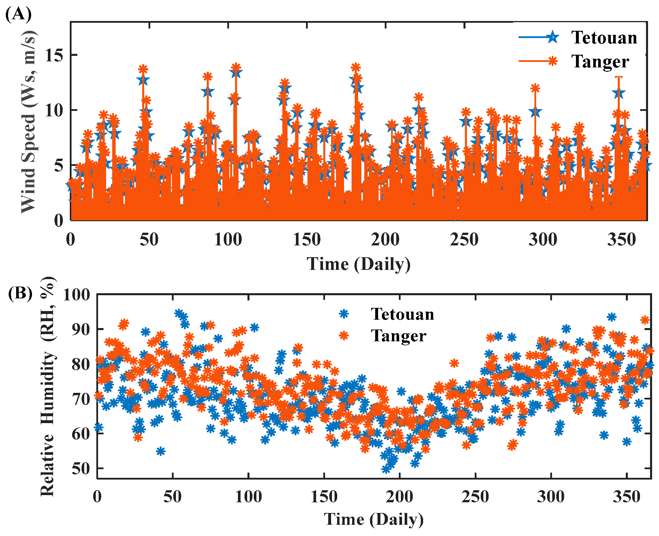
2.1. Data Collection and Study Sites
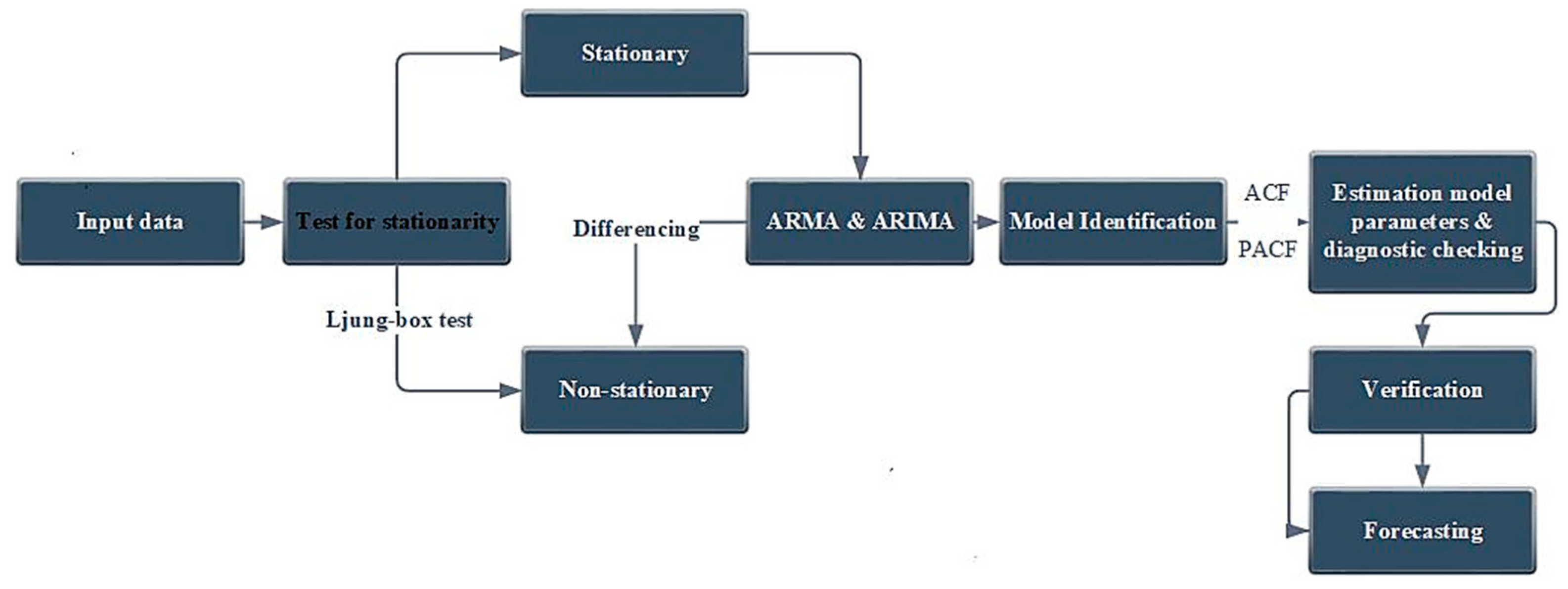
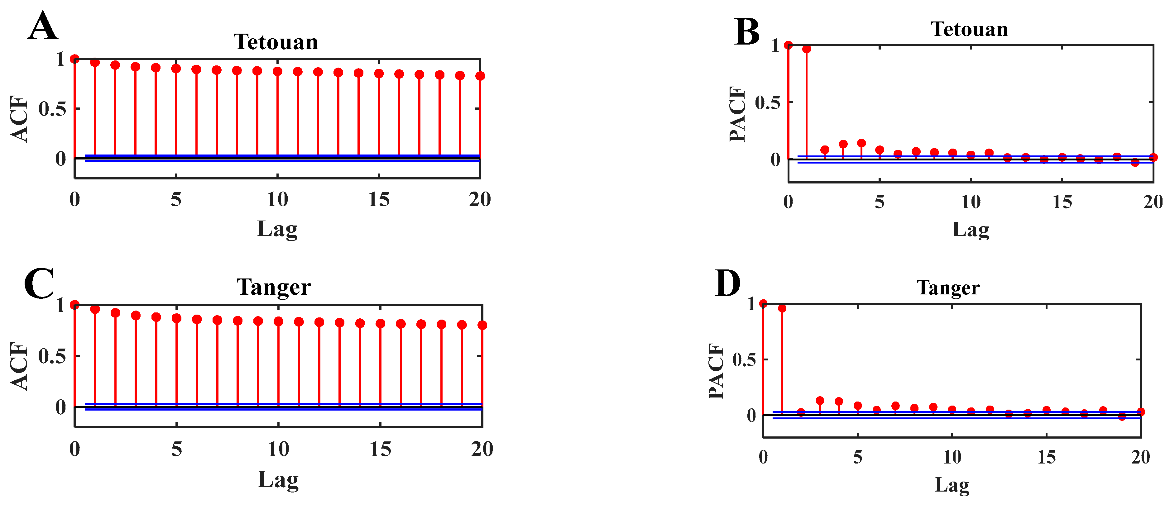
2.2. ARIMA and ARMA Model
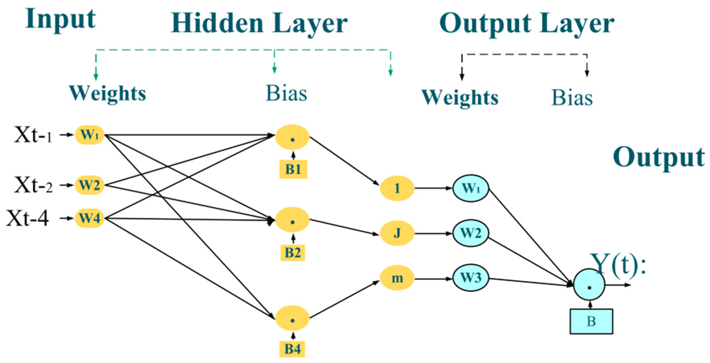
2.3. Artificial Neural Network Model (FFBP)
2.4. Hybrid Model
- -
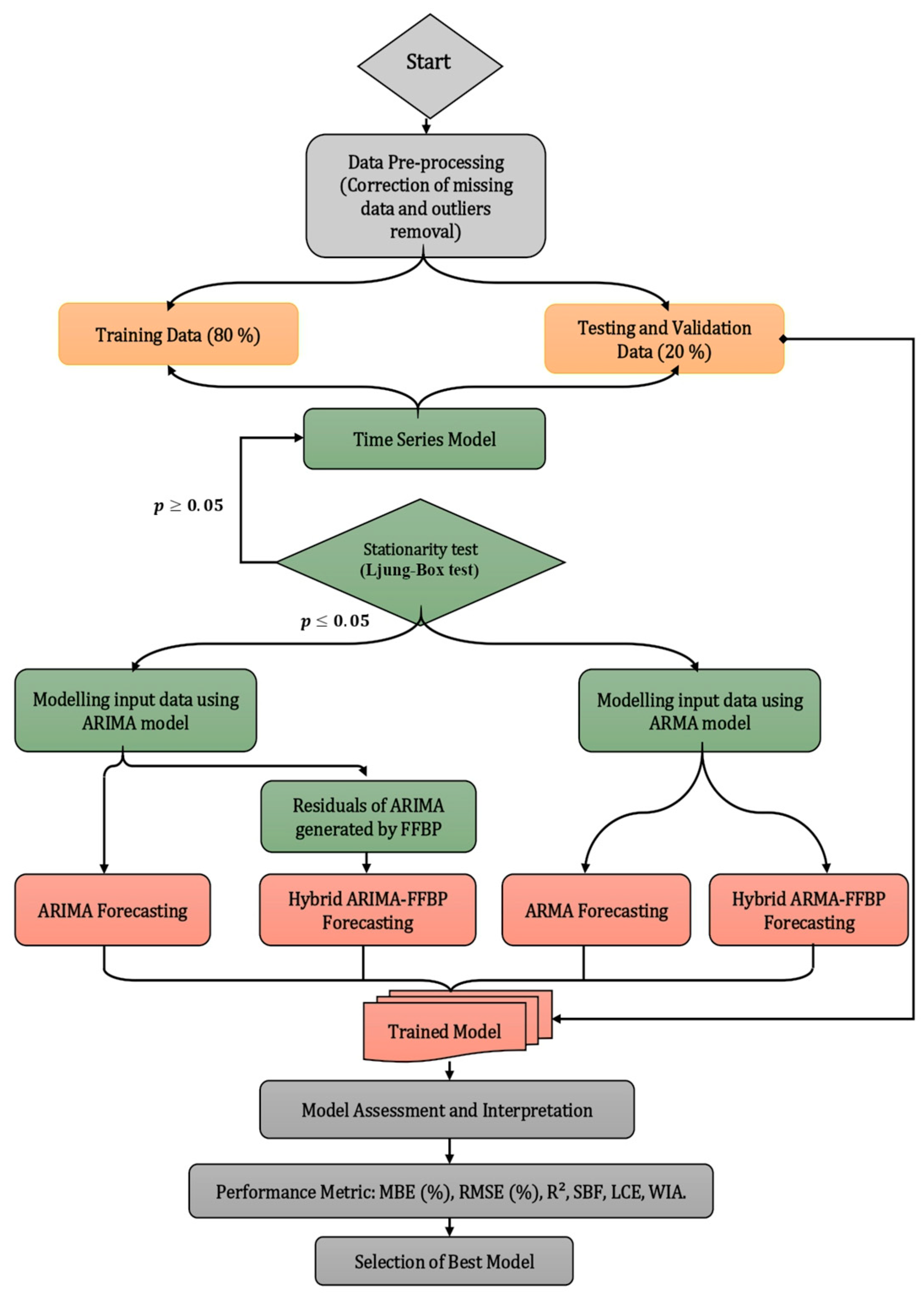
- Data pre-processing in section one (grey color) involves the collection of meteorological, computational, astronomical, and geographical data. These parameters require many corrections of missing data and outlier removal.
- -
- The application of multiple combinations of several input parameters in order to select the appropriate architecture executed in section two (gold color) was accomplished by splitting data into two steps, which are training data (80%), testing, and validation (20%) data.
- -
- The step of the training (green color) was operating the proposed methodologies. The input parameters were tested by using time series model stationarity (Ljung–Box test). After that, the data stationarity was implemented for ARIMA and ARMA models. In the case of the ARIMA model, that involves the residual generated by the FFBP model, which built the combined ARIMA and FFBP models.
- -
- The models were built and divided into simple (ARMA, ARIMA, and FFBP), and hybrid methods (hybrid ARMA-FFBP and hybrid ARIMA-FFBO models; orange color).
- -
- The obtained result (grey color) was evaluated and interpreted by using various statistical metrics in order to choose the best model, which presents the lowest value of MBE (%), RMSE (% Sd (%), AIC, and BIC and the highest values of R2, SBF, LCE, WIA.
2.5. Model Selection
2.6. Performance Criterion
3. Results and Discussion
4. Conclusions
Author Contributions
Funding
Data Availability Statement
Conflicts of Interest
References
- Suresh, M.; Meenakumari, R.; Panchal, H.; El Agouz, E.S.; Israr, M. An enhanced multiobjective particle swarm optimization algorithm for optimum utilization of hybrid renewable energy systems. Int. J. Ambient Energy 2020, 43, 2540–2548. [Google Scholar] [CrossRef]
- Ma, T.; Yang, H.; Lu, L.; Peng, J. Optimal design of an autonomous solar–wind-pumped storage power supply system. Appl. Energy 2015, 160, 728–736. [Google Scholar] [CrossRef]
- Belmahdi, B.; El Bouardi, A. Simulation and optimization of microgrid distributed generation: A case study of university abdelmalek essaâdi in Morocco. Procedia Manuf. 2020, 46, 746–753. [Google Scholar] [CrossRef]
- Mellit, A.; Pavan, A.M. A 24-h forecast of solar irradiance using artificial neural network: Application for performance prediction of a grid-connected PV plant at Trieste, Italy. Sol. Energy 2010, 84, 807–821. [Google Scholar] [CrossRef]
- Belmahdi, B.; El Bouardi, A. Solar potential assessment using PVsyst software in the northern zone of Morocco. Procedia Manuf. 2020, 46, 738–745. [Google Scholar] [CrossRef]
- Lan, H.; Zhang, C.; Hong, Y.-Y.; He, Y.; Wen, S. Day-ahead spatiotemporal solar irradiation forecasting using frequency-based hybrid principal component analysis and neural network. Appl. Energy 2019, 247, 389–402. [Google Scholar] [CrossRef]
- Louzazni, M.; Mosalam, H.; Khouya, A. A non-linear auto-regressive exogenous method to forecast the photovoltaic power output. Sustain. Energy Technol. Assess. 2020, 38, 100670. [Google Scholar] [CrossRef]
- Belmahdi, B.; Louzazni, M.; El Bouardi, A. A hybrid ARIMA–ANN method to forecast daily global solar radiation in three different cities in Morocco. Eur. Phys. J. Plus 2020, 135, 925. [Google Scholar] [CrossRef]
- Pereira, S.; Canhoto, P.; Salgado, R.; Costa, M.J. Development of an ANN based corrective algorithm of the operational ECMWF global horizontal irradiation forecasts. Sol. Energy 2019, 185, 387–405. [Google Scholar] [CrossRef]
- Koca, A.; Oztop, H.F.; Varol, Y.; Koca, G.O. Estimation of solar radiation using artificial neural networks with different input parameters for Mediterranean region of Anatolia in Turkey. Expert Syst. Appl. 2011, 38, 8756–8762. [Google Scholar] [CrossRef]
- Büyükşahin, Ü.Ç.; Ertekin, Ş. Improving forecasting accuracy of time series data using a new ARIMA-ANN hybrid method and empirical mode decomposition. Neurocomputing 2019, 361, 151–163. [Google Scholar] [CrossRef] [Green Version]
- Kazantzidis, A.; Nikitidou, E.; Salamalikis, V.; Tzoumanikas, P.; Zagouras, A. New challenges in solar energy resource and forecasting in Greece. Int. J. Sustain. Energy 2018, 37, 428–435. [Google Scholar] [CrossRef]
- Liu, Y.; Qin, H.; Zhang, Z.; Pei, S.; Wang, C.; Yu, X.; Jiang, Z.; Zhou, J. Ensemble spatiotemporal forecasting of solar irradiation using variational Bayesian convolutional gate recurrent unit network. Appl. Energy 2019, 253, 113596. [Google Scholar] [CrossRef]
- Fouilloy, A.; Voyant, C.; Notton, G.; Motte, F.; Paoli, C.; Nivet, M.L.; Guillot, E.; Duchaud, J.L. Solar irradiation prediction with machine learning: Forecasting models selection method depending on weather variability. Energy 2018, 165, 620–629. [Google Scholar] [CrossRef]
- Belmahdi, B.; Louzazni, M.; Akour, M.; Cotfas, D.T.; Cotfas, P.A.; El Bouardi, A. Long-term global solar radiation prediction in 25 cities in morocco using the FFNN-BP method. Front. Energy Res. 2021, 9, 733842. [Google Scholar] [CrossRef]
- Belmahdi, B.; Louzazni, M.; El Bouardi, A. Comparative optimization of global solar radiation forecasting using machine learning and time series models. Environ. Sci. Pollut. Res. 2021, 29, 14871–14888. [Google Scholar] [CrossRef]
- Mellit, A. Artificial Intelligence technique for modelling and forecasting of solar radiation data: A review. Int. J. Artif. Intell. Soft Comput. 2008, 1, 52–76. [Google Scholar] [CrossRef]
- López, G.; Batlles, F.J.; Tovar-Pescador, J. Selection of input parameters to model direct solar irradiance by using artificial neural networks. Energy 2005, 30, 1675–1684. [Google Scholar] [CrossRef]
- Lampinen, J.; Vehtari, A. Bayesian approach for neural networks—Review and case studies. Neural Netw. 2001, 14, 257–274. [Google Scholar] [CrossRef]
- Penny, W.D.; Roberts, S.J. Bayesian neural networks for classification: How useful is the evidence framework? Neural Netw. 1999, 12, 877–892. [Google Scholar] [CrossRef]
- Benvenuto, D.; Giovanetti, M.; Vassallo, L.; Angeletti, S.; Ciccozzi, M. Application of the ARIMA model on the COVID-2019 epidemic dataset. Data Brief 2020, 29, 105340. [Google Scholar] [CrossRef]
- Jamil, R. Hydroelectricity consumption forecast for Pakistan using ARIMA modeling and supply-demand analysis for the year 2030. Renew. Energy 2020, 154, 1–10. [Google Scholar] [CrossRef]
- Wang, W.; Chau, K.; Xu, D.; Chen, X.-Y. Improving forecasting accuracy of annual runoff time series using ARIMA based on EEMD decomposition. Water Resour. Manag. 2015, 29, 2655–2675. [Google Scholar] [CrossRef]
- Gibrilla, A.; Anornu, G.; Adomako, D. Trend analysis and ARIMA modelling of recent groundwater levels in the White Volta River basin of Ghana. Groundw. Sustain. Dev. 2018, 6, 150–163. [Google Scholar] [CrossRef]
- Bamisile, O.; Oluwasanmi, A.; Ejiyi, C.; Yimen, N.; Obiora, S.; Huang, Q. Comparison of machine learning and deep learning algorithms for hourly global/diffuse solar radiation predictions. Int. J. Energy Res. 2022, 46, 10052–10073. [Google Scholar] [CrossRef]
- Bamisile, O.; Cai, D.; Oluwasanmi, A.; Ejiyi, C.; Ukwuoma, C.C.; Ojo, O.; Mukhtar, M.; Huang, Q. Comprehensive assessment, review, and comparison of AI models for solar irradiance prediction based on different time/estimation intervals. Sci. Rep. 2022, 12, 9644. [Google Scholar] [CrossRef]
- Huang, L.; Kang, J.; Wan, M.; Fang, L.; Zhang, C.; Zeng, Z. Solar radiation prediction using different machine learning algorithms and implications for extreme climate events. Front. Earth Sci. 2021, 9, 596860. [Google Scholar] [CrossRef]
- Atique, S.; Noureen, S.; Roy, V.; Subburaj, V.; Bayne, S.; MacFie, J. Forecasting of total daily solar energy generation using ARIMA: A case study. In Proceedings of the 2019 IEEE 9th Annual Computing and Communication Workshop and Conference, CCWC 2019, Las Vegas, NV, USA, 7–9 January 2019; pp. 114–119. [Google Scholar] [CrossRef]
- Shams, M.B.; Haji, S.; Salman, A.; Abdali, H.; Alsaffar, A. Time series analysis of Bahrain’s first hybrid renewable energy system. Energy 2016, 103, 1–15. [Google Scholar] [CrossRef]
- Hussain, S.; Al Alili, A. Day ahead hourly forecast of solar irradiance for Abu Dhabi, UAE. In Proceedings of the 2016 4th IEEE International Conference on Smart Energy Grid Engineering, SEGE 2016, Oshawa, ON, Canada, 21–24 August 2016; pp. 68–71. [Google Scholar] [CrossRef]
- Gairaa, K.; Khellaf, A.; Messlem, Y.; Chellali, F. Estimation of the daily global solar radiation based on Box-Jenkins and ANN models: A combined approach. Renew. Sustain. Energy Rev. 2016, 57, 238–249. [Google Scholar] [CrossRef]
- Hassan, J. ARIMA and regression models for prediction of daily and monthly clearness index. Renew. Energy 2014, 68, 421–427. [Google Scholar] [CrossRef]
- Sulaiman, M.Y.; Wahab, M.A.; Sulaiman, Z.A. Analysis of residuals in daily solar radiation time series. Renew. Energy 1997, 11, 97–105. [Google Scholar] [CrossRef] [Green Version]
- Wang, Z.; Wang, F.; Su, S. Solar irradiance short-term prediction model based on BP neural network. Energy Procedia 2011, 12, 488–494. [Google Scholar] [CrossRef] [Green Version]
- Vu, K.M. The ARIMA and VARIMA Time Series: Their Modelings, Analyses and Applications; AuLac Technologies: Ottawa, ON, Canada, 2007. [Google Scholar]
- Chatfield, C.; Xing, H. The Analysis of Time Series: An Introduction with R, 7th ed.; CRC Press: Boca Raton, FL, USA; Taylor & Francis Group: Abingdon, UK, 2019. [Google Scholar]
- Tsay, R.S. Analysis of Financial Time Series; Wiley: Hoboken, NJ, USA, 2010. [Google Scholar]
- Sansa, I.; Boussaada, Z.; Bellaaj, N.M. Solar radiation prediction using a novel hybrid model of ARMA and NARX. Energies 2021, 14, 6920. [Google Scholar] [CrossRef]
- Shadab, A.; Said, S.; Ahmad, S. Box–Jenkins multiplicative ARIMA modeling for prediction of solar radiation: A case study. Int. J. Energy Water Resour. 2019, 3, 305–318. [Google Scholar] [CrossRef]
- Akaike, H. Information Theory and an Extension of the Maximum Likelihood Principle; Springer: New York, NY, USA, 1998; pp. 199–213. [Google Scholar] [CrossRef]
- Belmahdi, B.; Louzazni, M.; El Bouardi, A. One month-ahead forecasting of mean daily global solar radiation using time series models. Optik 2020, 219, 165207. [Google Scholar] [CrossRef]
- McQuarrie, A.D.R.; Tsai, C.-L. Regression and Time Series Model Selection; World Scientific: Singapore, 1998. [Google Scholar]
- Somvanshi, V.K.; Pandey, O.P.; Agrawal, P.K.; Kalanker, N.; Prakash, M.R.; Chand, R. Modelling and prediction of rainfall using artificial neural network and ARIMA techniques. J. Ind. Geophys. Union 2006, 10, 141–151. [Google Scholar]
- Sudheer, K.P.; Gosain, A.K.; Ramasastri, K.S. A data-driven algorithm for constructing artificial neural network rainfall-runoff models. Hydrol. Process. 2002, 16, 1325–1330. [Google Scholar] [CrossRef]
- Hammerstrom, D. Working with neural networks. IEEE Spectr 1993, 30, 46–53. [Google Scholar] [CrossRef]
- Louzazni, M.; Khouya, A.; Amechnoue, K.; Mussetta, M.; Crăciunescu, A. Comparison and evaluation of statistical criteria in the solar cell and photovoltaic module parameters’ extraction. Int. J. Ambient Energy 2020, 41, 1482–1492. [Google Scholar] [CrossRef]
- Al-Dahidi, S.; Ayadi, O.; Adeeb, J.; Louzazni, M. Assessment of artificial neural networks learning algorithms and training datasets for solar photovoltaic power production prediction. Front. Energy Res. 2019, 7, 130. [Google Scholar] [CrossRef] [Green Version]
- Jaihuni, M.; Basak, J.K.; Khan, F.; Okyere, F.G.; Arulmozhi, E.; Bhujel, A.; Park, J.; Hyun, L.D.; Kim, H.T. A partially amended hybrid bi-gru—ARIMA model (PAHM) for predicting solar irradiance in short and very-short terms. Energies 2020, 13, 435. [Google Scholar] [CrossRef] [Green Version]
- Mukhtar, M.; Oluwasanmi, A.; Yimen, N.; Qinxiu, Z.; Ukwuoma, C.C.; Ezurike, B.; Bamisile, O. Development and comparison of two novel hybrid neural network models for hourly solar radiation prediction. Appl. Sci. 2022, 12, 1435. [Google Scholar] [CrossRef]
- Huang, X.; Zhang, C.; Li, Q.; Tai, Y.; Gao, B.; Shi, J. A Comparison of hour-ahead solar irradiance forecasting models based on LSTM network. Math. Probl. Eng. 2020, 2020, 4251517. [Google Scholar] [CrossRef]


| References | Simple and Combined Modeling for Short-Term and Long-Term Prediction of Solar Radiation |
|---|---|
| [28] | Seasonal ARIMA (0, 1, 2) (1, 0, 1) 30 was found to be a suitable model for predicting daily solar radiation at Reese Research Centre of Lubbock, Texas |
| [29] | ARIMA (1, 0, 0) was found reasonable in capturing the autocorrelative structures of the daily average of solar irradiance in Awali, Kingdom of Bahrain. |
| [30] | Non-seasonal ARIMA (2, 1, 3) was trained to predict day-ahead hourly global horizontal irradiance (GHI) in Abu Dhabi. |
| [8] | Hybrid ARIMA-backed propagation does not outperform ARIMA for hourly solar irradiance from National Solar Radiation Database (NRSDB) site from 2008 to 2009. |
| [31] | ARMA (2, 0) and ARMA (4, 0) were identified as appropriate models combined with ANN for the prediction of daily global solar radiation. |
| [32] | ARIMA (2, 1, 1) was developed for the prediction of the daily clearness index In Abu Dhabi. |
| [33] | Employed ARMA, which revealed that the residuals were best estimated by non-seasonal ARMA (2, 0) for daily solar radiation data over four locations in Malaysia. |
| [34] | Employed ANN-BP neural network and multilayered feed-forward neural network |
| Cities | TAO (KWh/m2/Day) | Kt | Tmean (°C) | Tmax (°C) | Tmin (°C) | Tratio (°C) | Longitude (Degree) | Latitude (Degree) | Altitude (Degree) | ||||
|---|---|---|---|---|---|---|---|---|---|---|---|---|---|
| Tangier | 5.92 | 0.681 | 17.429 | 21.8 | 13.3 | 8.6 | 1.5878 | 73.542 | 4.708 | 12.338 | −5.9 | 35.733 | 21 |
| Tetouan | 4.909 | 0.653 | 18.671 | 22.4 | 15.5 | 7.1 | 1.423 | 70.08 | 4.263 | 12.306 | −5.33 | 35.58 | 10 |
| Cities | ARMA Models | Parameters | Estimation | Standard Error | TS Statistic | p-Value |
|---|---|---|---|---|---|---|
| Tetouan | ARMA (10 0 0) | AR{1} | 0.39838 | 0.044196 | 9.0139 | 1.989410−19 |
| AR{2} | −0.14705 | 0.054537 | −2.6963 | 0.0070107 | ||
| AR{3} | 0.10918 | 0.054265 | 2.012 | 0.044216 | ||
| AR{4} | 0.034376 | 0.059844 | 0.57443 | 0.56568 | ||
| AR{5} | 0.10994 | 0.059868 | 1.8364 | 0.066304 | ||
| AR{6} | 0.096692 | 0.056285 | 1.7179 | 0.085814 | ||
| AR{7} | 0.16186 | 0.055111 | 2.9371 | 0.0033132 | ||
| AR{8} | 0.053943 | 0.049207 | 1.0962 | 0.27298 | ||
| AR{9} | 0.098247 | 0.054629 | 1.7985 | 0.072105 | ||
| AR{10} | 0.050805 | 0.051959 | 0.97779 | 0.32818 | ||
| Tangier | ARMA (16 0 0) | AR{1} | 0.38961 | 0.043978 | 8.8593 | 8.053110−19 |
| AR{2} | 0.06638 | 0.057461 | 1.1552 | 0.248 | ||
| AR{3} | 0.23474 | 0.053071 | 4.4231 | 9.73110−6 | ||
| AR{4} | −0.0063764 | 0.062151 | −0.1026 | 0.91828 | ||
| AR{5} | 0.061862 | 0.061564 | 1.0048 | 0.31498 | ||
| AR{6} | 0.083309 | 0.054007 | 1.5426 | 0.12293 | ||
| AR{7} | −0.00041644 | 0.06213 | −0.006702 | 0.99465 | ||
| AR{8} | 0.034286 | 0.066352 | 0.51674 | 0.60534 | ||
| AR{9} | 0.0060834 | 0.055003 | 0.1106 | 0.91193 | ||
| AR{10} | −0.05637 | 0.054918 | −1.0264 | 0.30469 | ||
| AR{11} | −0.046987 | 0.059012 | −0.79623 | 0.4259 | ||
| AR{12} | 0.10782 | 0.047812 | 2.255 | 0.024135 | ||
| AR{13} | −0.04943 | 0.049427 | −1.0001 | 0.31728 | ||
| AR{14} | 0.0078379 | 0.052373 | 0.14966 | 0.88104 | ||
| AR{15} | −0.0036433 | 0.054602 | −0.066725 | 0.9468 | ||
| AR{16} | 0.16003 | 0.048865 | 3.2749 | 0.0010569 |
| Cities | ARMA Models | Parameters | Estimation | Standard Error | TS Statistic | p-Value |
|---|---|---|---|---|---|---|
| Tetouan | ARIMA (2.1.0) | AR{1} | −0.03912 | 0.009215 | −4.2452 | 0.21838 |
| AR{2} | −0.15594 | 0.012313 | −12.6654 | 0.92005 | ||
| Tangier | ARIMA (2.2.0) | AR{1} | −0.58945 | 0.009849 | −59.8438 | 0.16258 |
| AR{2} | −0.33481 | 0.010903 | −30.7077 | 0.44859 |
| Cities | Measured Data | FFBP Architecture | Coefficient of Variation (CV) | RMSE (%) |
|---|---|---|---|---|
| Tetouan | FFBP (1 × 2 × 1) | 0.575 | 0.5957 | |
| FFBP (2 × 2 × 1) | 0.571 | 0.5119 | ||
| FFBP (3 × 2 × 1) | 0.562 | 0.5045 | ||
| FFBP (4 × 2 × 1) | 0.555 | 0.5002 | ||
| FFBP (5 × 2 × 1) | 0.526 | 0.5002 | ||
| FFBP (6 × 2 × 1) | 0.519 | 0.4975 | ||
| FFBP (7 × 2 × 1) | 0.492 | 0.4966 | ||
| FFBP (8 × 2 × 1) | 0.473 | 0.4935 | ||
| FFBP (9 × 2 × 1) | 0.457 | 0.4928 | ||
| FFBP (10 × 2 × 1) | 0.440 | 0.4915 | ||
| FFBP (11 × 2 × 1) | 0.435 | 0.4901 | ||
| FFBP (12 × 2 × 1) | 0.426 | 0.489 | ||
| Tangier | FFBP (1 × 2 × 1) | 0.467 | 0.5119 | |
| FFBP (2 × 2 × 1) | 0.453 | 0.5045 | ||
| FFBP (3 × 2 × 1) | 0.448 | 0.5002 | ||
| FFBP (4 × 2 × 1) | 0.442 | 0.5002 | ||
| FFBP (5 × 2 × 1) | 0.434 | 0.4975 | ||
| FFBP (6 × 2 × 1) | 0.426 | 0.4966 | ||
| FFBP (7 × 2 × 1) | 0.426 | 0.4957 | ||
| FFBP (8 × 2 × 1) | 0.419 | 0.4935 | ||
| FFBP (9 × 2 × 1) | 0.410 | 0.4928 | ||
| FFBP (10 × 2 × 1) | 0.409 | 0.4895 | ||
| FFBP (11 × 2 × 1) | 0.399 | 0.4395 | ||
| FFBP (12 × 2 × 1) | 0.382 | 0.406 |
| Cities | Models | MBE | MBE (%) | RMSE | RMSE (%) | Sd | Sd (%) | R2 | SBF | LCE | WIA | BIC | AIC |
|---|---|---|---|---|---|---|---|---|---|---|---|---|---|
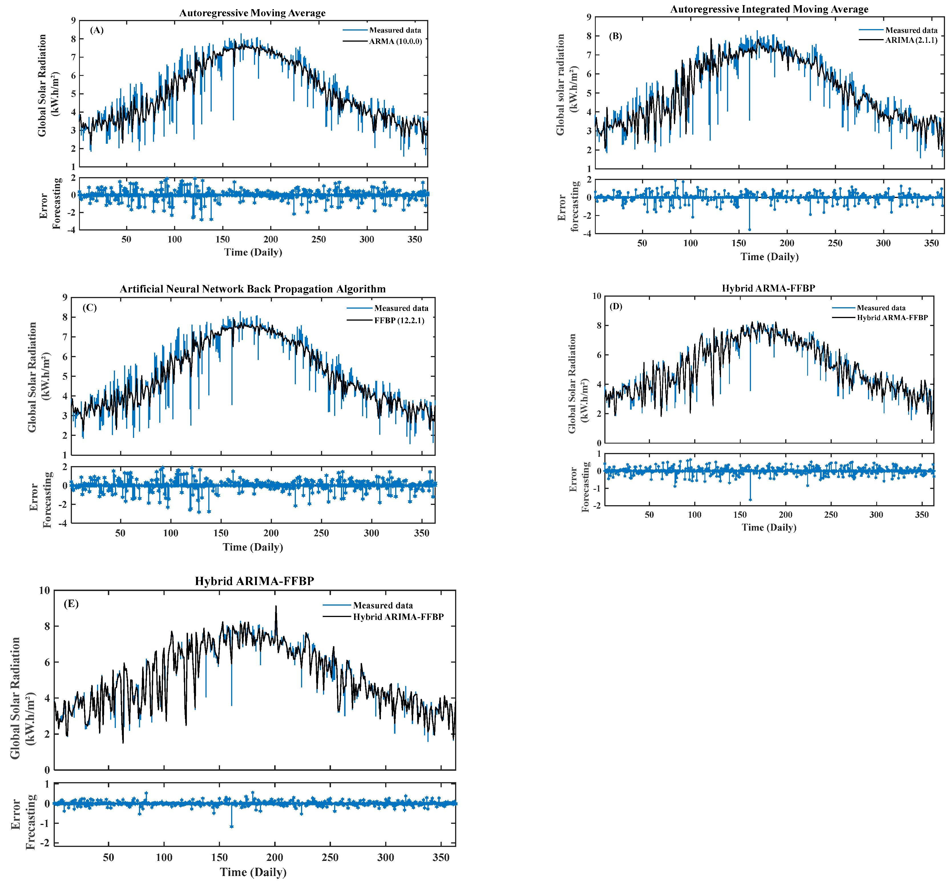
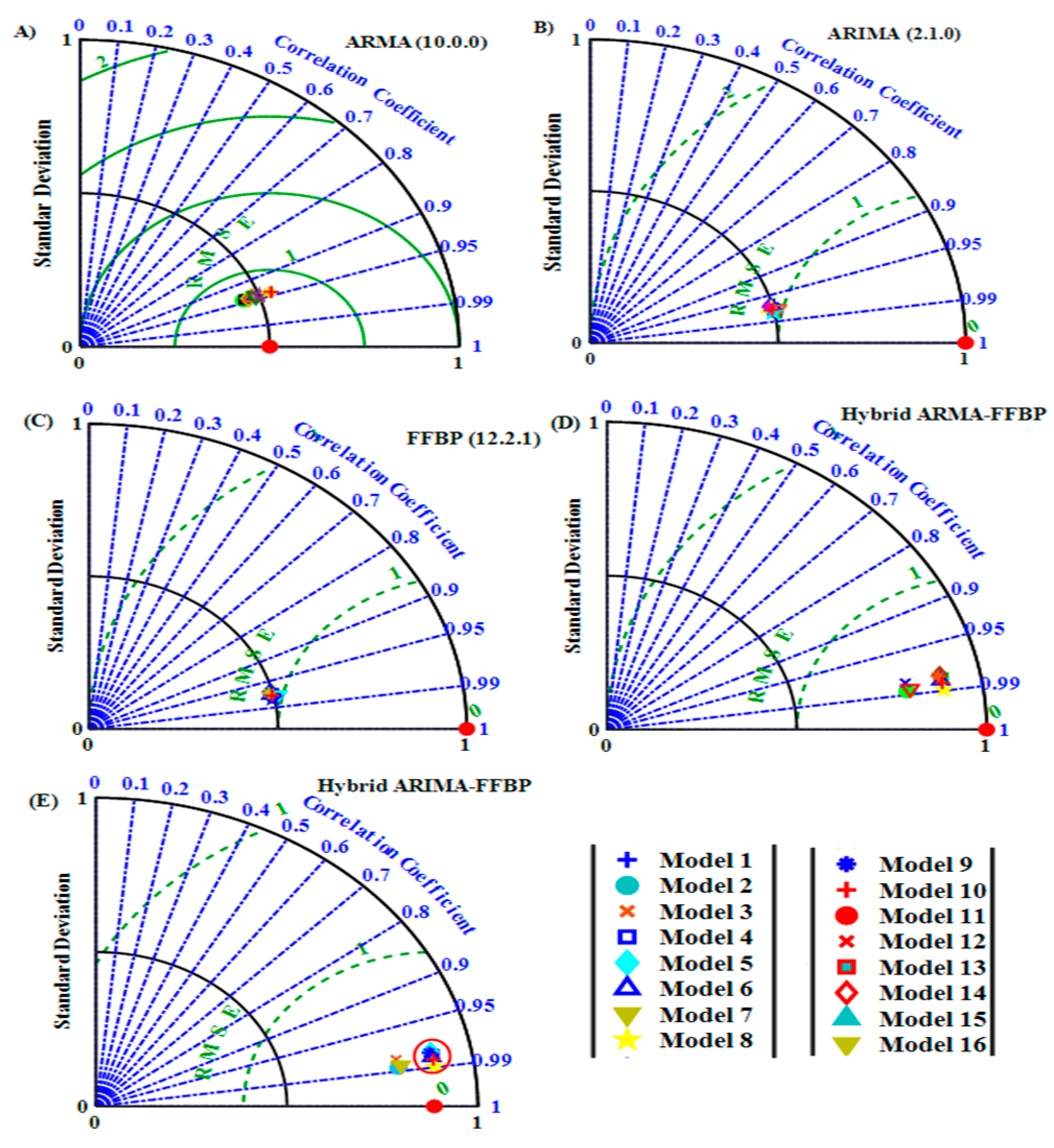
| Tetouan | ARIMA (2, 1, 0) | 0.0817 | 0.0839 | 0.80540 | 16.6421 | 0.7554 | 12.6704 | 0.9628 | 0.8998 | 0.9253 | 0.9491 | 1038.213 | 991.7475 |
| ARMA (10, 0, 0) | 0.1665 | 0.1098 | 1.0671 | 20.1083 | 0.9642 | 15.6709 | 0.9472 | 0.8915 | 0.9169 | 0.9689 | 1298.657 | 1051.867 | |
| FFBP (12, 2, 1) | 0.0529 | 0.0364 | 0.5119 | 10.0253 | 0.5098 | 9.98521 | 0.9878 | 0.9098 | 0.9498 | 0.9887 | 991.3442 | 890.6528 | |
| Hybrid ARMA–FFBP | 0.0376 | 0.0301 | 0.4871 | 9.98512 | 0.5001 | 9.10862 | 0.9890 | 0.9148 | 0.9580 | 0.9910 | 862.0175 | 810.6171 | |
| Hybrid ARIMA–FFBP | 0.0298 | 0.0297 | 0.4091 | 9.6917 | 0.4678 | 8.67911 | 0.9931 | 0.9163 | 0.9641 | 0.9945 | 792.8625 | 756.3418 | |
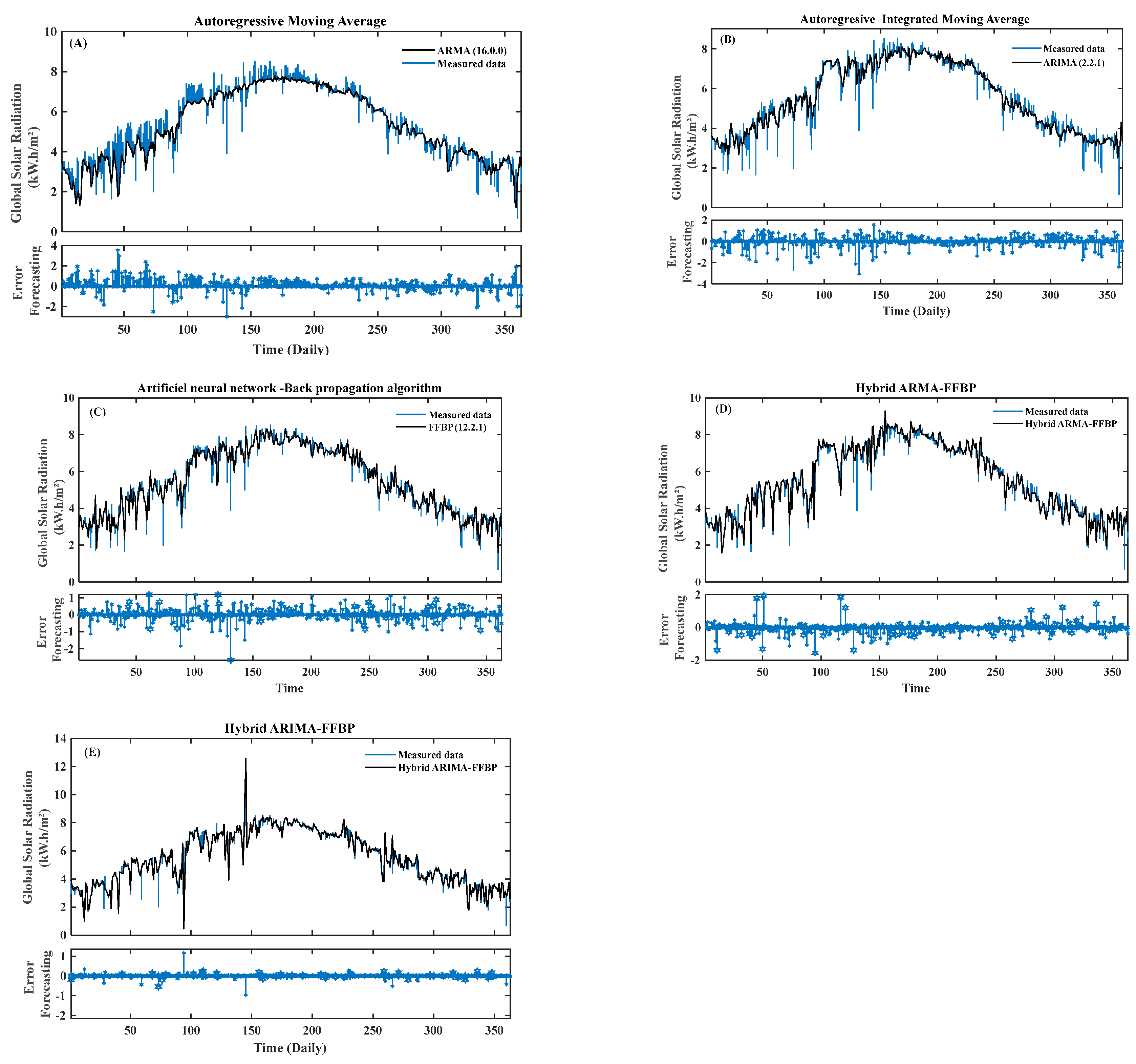
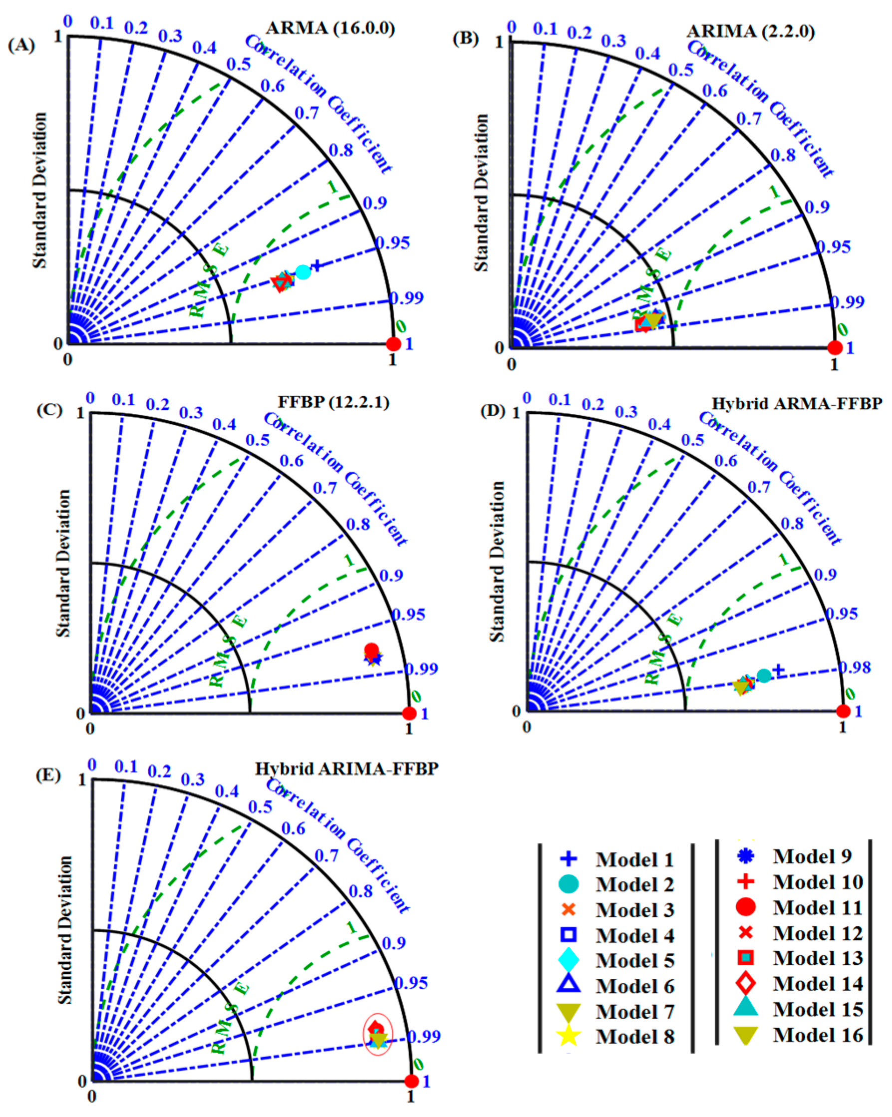
| Tangier | ARIMA (2, 2, 0) | 0.0042 | 0.06301 | 0.606335 | 17.41963 | 0.90689 | 12.42982 | 0.9744 | 0.8435 | 0.8954 | 0.9686 | 857.8941 | 788.5028 |
| ARMA (16, 0, 0) | 0.0709 | 0.10072 | 0.89561 | 23.0964 | 0.99875 | 16.6418 | 0.9601 | 0.8074 | 0.8638 | 0.9487 | 1096.819 | 976.183 | |
| FFBP (12, 2, 1) | 0.0517 | 0.03092 | 0.47834 | 10.3863 | 0.79265 | 7.40331 | 0.9834 | 0.8671 | 0.9145 | 0.9891 | 835.265 | 645.765 | |
| Hybrid ARMA–FFBP | 0.0401 | 0.02564 | 0.39876 | 9.68745 | 0.71563 | 7.01577 | 0.9888 | 0.9188 | 0.9615 | 0.9981 | 803.465 | 598.615 | |
| Hybrid ARIMA–FFBP | 0.0222 | 0.02101 | 0.30762 | 9.06742 | 0.69426 | 6.87613 | 0.9901 | 0.9296 | 0.9696 | 0.9939 | 765.091 | 504.816 |
Disclaimer/Publisher’s Note: The statements, opinions and data contained in all publications are solely those of the individual author(s) and contributor(s) and not of MDPI and/or the editor(s). MDPI and/or the editor(s) disclaim responsibility for any injury to people or property resulting from any ideas, methods, instructions or products referred to in the content. |
© 2023 by the authors. Licensee MDPI, Basel, Switzerland. This article is an open access article distributed under the terms and conditions of the Creative Commons Attribution (CC BY) license (https://creativecommons.org/licenses/by/4.0/).
Share and Cite
Belmahdi, B.; Louzazni, M.; Marzband, M.; El Bouardi, A. Global Solar Radiation Forecasting Based on Hybrid Model with Combinations of Meteorological Parameters: Morocco Case Study. Forecasting 2023, 5, 172-195. https://doi.org/10.3390/forecast5010009
Belmahdi B, Louzazni M, Marzband M, El Bouardi A. Global Solar Radiation Forecasting Based on Hybrid Model with Combinations of Meteorological Parameters: Morocco Case Study. Forecasting. 2023; 5(1):172-195. https://doi.org/10.3390/forecast5010009
Chicago/Turabian StyleBelmahdi, Brahim, Mohamed Louzazni, Mousa Marzband, and Abdelmajid El Bouardi. 2023. "Global Solar Radiation Forecasting Based on Hybrid Model with Combinations of Meteorological Parameters: Morocco Case Study" Forecasting 5, no. 1: 172-195. https://doi.org/10.3390/forecast5010009
APA StyleBelmahdi, B., Louzazni, M., Marzband, M., & El Bouardi, A. (2023). Global Solar Radiation Forecasting Based on Hybrid Model with Combinations of Meteorological Parameters: Morocco Case Study. Forecasting, 5(1), 172-195. https://doi.org/10.3390/forecast5010009