Abstract
The adequate modeling and estimation of solar radiation plays a vital role in designing solar energy applications. In fact, unnecessary environmental changes result in several problems with the components of solar photovoltaic and affects the energy generation network. Various computational algorithms have been developed over the past decades to improve the efficiency of predicting solar radiation with various input characteristics. This research provides five approaches for forecasting daily global solar radiation (GSR) in two Moroccan cities, Tetouan and Tangier. In this regard, autoregressive integrated moving average (ARIMA), autoregressive moving average (ARMA), feed forward back propagation neural networks (FFBP), hybrid ARIMA-FFBP, and hybrid ARMA-FFBP were selected to compare and forecast the daily global solar radiation with different combinations of meteorological parameters. In addition, the performance in three approaches has been calculated in terms of the statistical metric correlation coefficient (R2), root means square error (RMSE), stand deviation (σ), the slope of best fit (SBF), legate’s coefficient of efficiency (LCE), and Wilmott’s index of agreement (WIA). The best model is selected by using the computed statistical metric, which is present, and the optimal value. The R2 of the forecasted ARIMA, ARMA, FFBP, hybrid ARIMA-FFBP, and ARMA-FFBP models is varying between 0.9472% and 0.9931%. The range value of SPE is varying between 0.8435 and 0.9296. The range value of LCE is 0.8954 and 0.9696 and the range value of WIA is 0.9491 and 0.9945. The outcomes show that the hybrid ARIMA–FFBP and hybrid ARMA–FFBP techniques are more effective than other approaches due to the improved correlation coefficient (R2).
1. Introduction
The global consideration of renewable energy sources such as solar energy, wind, hydro, and biomass has remarkably increased in terms of sustainable energy due to the reduction of fossil fuels. In this regard, the implementation of solar energy sources has widely focused on the use of photovoltaic (PV) systems, thermal solar energy, and concentrated solar energy [1]. In particular, the emergence of renewable energy has enhanced solar radiation forecasting in the activity and management of the modern smart grid, with renewable energy generation [2,3].
Solar radiation forecasting has become crucial to accurately predict the efficiency of solar energy conversion systems and ensure the electrical grid’s reliability and safety. Specifically, global solar radiation is the most critical aspect of solar energy, which is essential for implementing renewable, solar energy systems, and PV system sizing [4,5]. Moreover, a precise understanding of solar radiation could optimize the accuracy of the electricity network and increase the efficiency of the smart grid. Therefore, appropriate solar radiation forecasting significantly improves solar energy usage, rises the economic losses due to electrical constraints, and maximizes the return on investment in photovoltaic grids [6]. However, solar radiation is considered one of the prime resources and it plays a significant role in the foreseeable future, particularly in developing countries.
The forecasting of solar radiation was commonly discussed in the literature review. Several researchers have categorized the forecasting solar radiation into four types such as very-short-, short-, medium- and long-forecasting [7]. However, the appropriate approaches are required to improve solar radiation forecasting model accuracy and reduce the negative effects of system fluctuations. These are structured in two main methods, namely, the time series statistical method and the physical techniques, and the combination of the above techniques called the hybrid techniques [8]. The selected techniques are depending entirely on the forecasting horizon, available data information, and locations. In addition, the physical techniques are based on various equations, which describe the transmission phenomena and thermodynamic mechanisms, occurring in the atmosphere and on the surface of the earth. However, the equations become more complex when additional variables are added such as temperature, wind speed, dust, and humidity [9]. The forecast accuracy of the physical techniques mainly depends on the accuracy of the collected data and various information about the location. Further, the time series statistical technique is purely based on the relationship between the past values of the weather parameters and the solar radiation that are identified and used in the forecasting process. This could include forecasting methods such as artificial neural networks, vector support machines, Markov chains, auto-regressive models, or regression models. Additionally, the time series could be described as a series of measurements collected over time at regular intervals; it is flexible and requires fewer data inputs, resulting in simple implementation and less cost. However, the main limitation of forecasting time series is the absence of deterministic causes [10]. According to this background, numerous papers have developed various models and techniques with the times series analysis, based on artificial neural networks (ANNs) [11]. In [12], have presented a brief overview of the different techniques to determine their source and forecast solar radiation using ANNs in Greece. Further, the results elaborate that the geographical pattern and the different climatic conditions enhance the cloud’s temporal and spatial variability. A new model has been developed based on the ensemble of spatiotemporal deep learning models and variational Bayesian inference which uses spatiotemporal information to forecast solar radiation in the literature [13]. In [14], the authors compared eleven statistical and machine learning models for hourly solar radiation forecasting based on three meteorological locations with different collected data, and they explain that the precision and performance of each model are related to the variation of both the meteorological location and solar radiation information. In addition, the efficiency of the models was compared in terms of the statistical metrics named normalized root mean square error (RMSE), mean absolute error (MAE), and skill score. For weak variability, the auto-regressive moving average and multi-layer perceptron are the best predictors. The feedforward backpropagation algorithm was used by [15] to predict daily global solar radiation in 25 cities around the kingdom of Morocco. Several meteorological astronomical and geographical coordinates were employed as input data to predict the outcoming output. Multiple combination parameters were adopted to select the most suitable configuration with optimal input data for each study location. According to statistical metrics, the obtained result is, respectively, twelve inputs for Er-Rachidia, Marrakech, Medilt, Taza, Oujda, Nador, Tetouan, Tangier, Al-Auin, Dakhla, Settat, and Safi, seven inputs for Fes, Ifrane, Beni-Mellal, and Meknes; six inputs for Agadirand Rabat; five inputs for Sidi Ifni, Essaouira, Casablanca, and Kenitra; and four inputs for Ouarzazate, Larache, and Al-Hoceima. In terms of accuracy, the R2 of the selected best inputs parameters varies between 0.9860% and 0.9920%, with the range value of MBE (%) being from −0.1076% to −0.5931%, the RMSE between 0.1990 and 0.4580%, the range value of the NRMSE is between 0.0355 and 0.8938, and the lowest value of the MAPE is between 0.0019 and 0.0060%. This technique could be used to predict other parameters for locations where measurement instrumentation is unavailable or costly to obtain. In the meantime, the authors of [16] presented a comparative optimization of daily global solar radiation forecasting with different machine learning and time series methods. The selected methods are compared with the persistence technique and measured data. Several statistical metrics are assessed to obtain the most appropriate method, which presents the lowest value accuracy. The select result is, respectively, the RMSE (%) and MBE (%) values of several models employed in this study, and were computed to be mostly positive. The range value of the selected model measured by RMSE (%) and MBE (%) varied between 4.64% to 8.87% and 6% to 22.93%. Based on all statistical metrics, the lower value of the selected model corresponds to the neural FFBP (6 × 10 × 1) in comparison with the other models. The appropriate one performs well and is close to the measured data. The authors of [17] presented a complete and detailed synthesis of solar radiation modeling, forecasting, and solar radiation data using artificial intelligence methods: ANN, fuzzy logic, genetic algorithm, expert system, and a hybrid method. It is proven that solar radiation is a vital factor in PV system performance and sizing. The same researchers have presented a combination of the above methods for generating horizontal global solar radiation by combining ANN and library of Markov transition metrics (MTM) approaches based on three-parameter coordinates (longitude, altitude, and latitude) and the data were collected from a data basis of 60 stations in Algeria over 9 years. This prediction is comparatively accurate related to the relative Root Mean Square Error (RMSE), which is less than 8.2%. On other hand, López et al. [18] have chosen the automatic relevance determination method (ARD) based on the ANN model to select the relevant input parameters in direct normal solar irradiance forecasting. Clearness index and relative air mass were considered the most important input parameters to the neural network. According to J. Lampinen et al. [19], Penny et al. [20], and B. Belmahdi et al. [8], the ARD and ANN are the priority distribution on the network weights and determine the most relevant input parameters by introducing a hyperparameter for each input unit of the ANN. In ANNs, the important prior distribution of the network weights is controlled by the hyperparameters. Here, the ANN is presented with training data, and posterior weight distribution and hyperparameters are calculated using the Bayes rules.
Recently, time series forecasting models have taken the attention of researchers in different fields for their power and ability to forecast complex systems [11]. Especially, the autoregressive integrated moving average (ARIMA) was utilized in the COVID-2019 pandemic [21], hydroelectricity [22], agriculture [23], and groundwater-based irrigation [24]. Generally, ARIMA models are an integration of autoregressive models (AR) and moving average models (MA), which have proven reasonable precision in the forecasting of stationary time-series information. Further, it is strongly assumed that the prospective data values are linearly dependent on present and past data values. However, several real-world time series data result from dynamic non-linear structures that cannot be accurately modeled by ARIMA. Consequently, artificial neural networks (ANNs) are considered the most commonly implemented algorithms for nonlinear time series modeling. In another word, the ANNs have a range of benefits with respect to ARIMA and other forecasting frameworks, which are capable of executing a dynamic non-linear function. Hence, the ANNs are capable of reconstructing every continuously measurable function with arbitrary desired accuracy [11]. Moreover, ANNs are flexibly data-driven in design, which ensures that ANN models could be modified with the characteristics of time series data information. Several studies have been carried out to compare the performance of machine learning (ML) and deep learning (DL) algorithms in forecasting solar radiation [25]. In some cases, ML algorithms have been found to be more accurate than DL algorithms [26], while DL methods have been found to be more accurate than ML algorithms in others [27]. In this context, Table 1 summarizes the difference between ARIMA and FFBP in solar radiation forecasting in various locations.

Table 1.
Selected studies on ARIMA and ANN modeling of solar radiation.
As a novel method for time series forecasting, hybrid ARIMA-FFBP and ARMA-FFBP models have been developed. FFBP is a sort of feed-forward neural network that employs log sigmoidal functions. In comparison to single models and other hybrid models like SARIMA-MLP, it has been observed that this hybrid technique increases accuracy and minimizes errors. These hybrid ARIMA-FFBP, and ARMA-FFBP models could be further deployed to forecast the future performance and energy capacity of solar energy systems. Here, both have accompanied a different combination of parameters for inputs to select the adequate model. In addition, the daily solar radiation data is collected from two cities called Tetouan and Tangier in northern Morocco. These locations are essential, as the solar energy intensities are utilized in the photovoltaic and thermal system and the region has the largest port in the Mediterranean area. Several statistical metrics are evaluated and calculated to validate the performance of the forecast values.
The rest of the paper is organized as follows. Section 2 contains collected data and the proposed methodology (forecasting method). Section 3 contains summarizes the statistical metric employed in this work. Section 4 contains the main finding and simulation results of the short-term forecasted daily global solar radiation. Lastly, the conclusion has been presented in Section 4.
2. Materials and Methods
2.1. Data Collection and Study Sites
The data was analyzed from the 1 January 2015 to the 31 December 2015, and conducted in a meteorological station installed on the rooftop of the Faculty of Science, Abdelmalek Essaadi Tetouan University (Figure 1). This station consists of pyranometers in Kipp & Zonen brands, model CM-11, for the measurement of global solar radiation. Another identical pyranometer and the shadow ring is operated to measure the diffuse solar radiation. The shadow ring has a width of 7.6 cm, a radius of 31 cm, an anemometer equipped with a wind vane with a horizontal axis turbine for the measurement of the wind speed, and direction—along with a Campbell scientific thermo-hygrometer containing two probes—to measure the temperature and the relative humidity. In addition, the local station uses a rain gauge to measure precipitation.
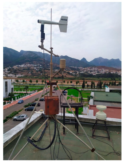
Figure 1.
Weather station of Abdelmalek Essaadi University, Faculty of Sciences, Morocco.
In Figure 2, we plot the daily range of the mean (Tmean), maximum (Tmax), and minimum (Tmin), temperature. The three-temperature dataset describes the timescale distribution of day-to-day temperature variations in the Tetouan and Tangier sites. The annual temperature variation reveals the succession of warm and cold periods over the year. The analysis is conducted for each day. The recorded Tmax was observed in the July period (38 °C for Tetouan and 36.6 °C for Tangier), while the Tmin was observed in the January period (6 °C for Tetouan and 2 °C for Tangier). The distribution of the Tmin is close to normal condition.
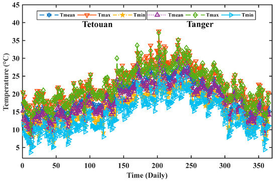
Figure 2.
Mean, maximum, and minimum daily temperature of Tetouan and Tangier sites.
Figure 3A,B show a representative behavior of the daily global solar radiation from January to December 2015 of the Tetouan and Tangier sites. The total solar radiation over the year was 18.63 MJ/m2 and 19.99 MJ/m2 with a standard deviation of 1.98 kW·h/m2 and 1.76 kW·h/m2 for the Tetouan and Tangier sites, respectively. In the warm period, the lowest solar radiation deviation was 1.106 kWh/m2 for the Tetouan site and 0.7375 kW·h/m2 for the Tangier site. The highest solar radiation deviation in the cold period was 7.48 kW·h/m2 and 7.413 kW·h/m for Tetouan and Tangier sites, respectively. As for month averages, the highest solar radiation months over the year were from May to July, while the lowest values were from December to January.
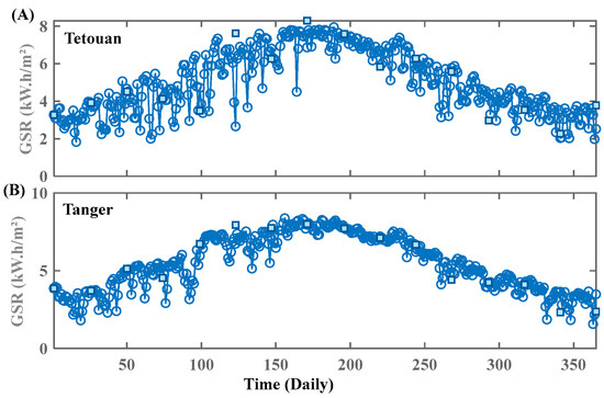
Figure 3.
(A,B) Daily global solar radiation distribution through a year of two sites.
In Figure 4A,B shows the daily wind speed (Ws) and relative humidity (Rh) over the year for the Tetouan and Tangier sites. The range value of wind speed varies by about 13.02 m/s and 13.3 m/s, respectively, for the Tetouan and Tangier sites. In the cold period, the highest relative humidity for the Tetouan and Tangier sites was 94.5% and 92.58%. In a warm period, the lowest relative humidity was 49.75% and 55.54%, respectively, for Tetouan and Tangier sites.
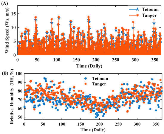
Figure 4.
(A) Distribution of daily wind speed (m/s) and (B) relative humidity (%).
The manipulations may require other types of meteorological parameters such as ambient temperature (T, °C; maximum, minimum, average, difference, and ratio), day number, day length, wind speed (Ws, m/s; average), relative humidity (RH,%), top of atmosphere radiation (TOA radiation), and geographic coordinates (Latitude, Altitude, and Longitude). These are exogenous data, whose periods and characteristics of measurements are summarized in Table 2.

Table 2.
Daily average inputs parameters data of Tetouan and Tanger sites.
2.2. ARIMA and ARMA Model
Generally, the ARIMA model could be recognized as the combination of several models named p, d, q, and AR (p) refers to the order of the autoregressive component. In fact, the I(d) integrated refers to the degree of differentiation involved, and MA(q) represents the order of the average movement of the components [35]. Moreover, the AR assumes that each value of the time series depends on the weighted production sum in the previous values and the most residual regression coefficient. An autoregressive model could be considered an autoregressive model of order (p) [36], which represents the previous (lagged) values of the dependent variable. MA is utilized to calculate the mean for a specified set of values and predict the following periods; MA (moving average) refers to the lagged error terms (i.e., residues) created by the model, which is represented by (q) [37]. The elements of the series could be affected by past errors (or a random shock), which are impossible to compute by the autoregressive component. The coupled AR(p) and MA (q) built an ARMA model which is commonly used in forecasting tacks [38]. The general ARIMA model p, d, q can be expressed as Equation (1):
Or in a general form as Equation (2):
where φi refers to the i-th term autoregressive parameter, θi refers to the ith term moving average parameter, c is the constant, et is defined as an error at time t, Bp refers to the p-th order backward shift operator, and X(t) is defined as a time series value at time t.
The first step in ARIMA and ARMA construction is to identify the time series stationary data as presented in Figure 5, and then significant seasonality in the time series. The assumptions which were accounted for in the ARIMA model are that the time series should be stationary, the flow data must be separated to secure the sequence stationary, the data should vary continuously, and the data has consisted of a logarithmic transition to rendering the variance stable to accommodate the stationary variability. In addition, the two methods which were deployed in the pattern recognition process are the sequence of correlograms called the autocorrelation (ACF) function and the partial autocorrelation function [39,40,41]. The ACF and PACF are considered the most important elements of time series analysis and forecasting. In particular, the ACF determines the amount of the linear dependency around measurements in the time series, while the PACF enables the calculation of the number of autoregressive terms necessary to demonstrate the time lag characteristics. Moreover, the Akaike Information Criterion was used as a provided tool to select the optimal AIC, where the lowest AIC was identified as a parsimonious model [39,40,42].
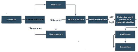
Figure 5.
Flowchart of the proposed Autoregressive Integrated Moving Average modeling of daily.
2.3. Artificial Neural Network Model (FFBP)
Neural networks are approximately similar to the human brain’s computing and create awareness of basic processing units called neurons. Neurons are divided into layers, and synaptic connections (weight) interconnect the neighboring layers. In particular, it is possible to distinguish three separate types of layers: the input layer, which connects the input information; the output layer, which generates the final output; and one or more hidden layers, which serve as intermediate computational layers between input and output [43]. In addition, the input values are measured by the first weights of the information exchange. Hence, the products are applied to the neuron with a particular parameter designated bias. This is utilized to extend the total number of the products over a reasonable range by becoming inputs for hidden layer nodes, which attach a non-linear activation structure (a sigmoid unit) to the total above-generated hidden node. These signals are interpreted in the same manner through the corresponding hidden layers (if any) or the output layer, producing the output of the network, which is illustrated in Figure 6.
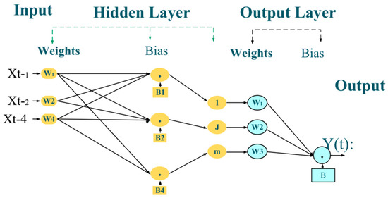
Figure 6.
FFBP neural network topology.
The connection between the output Y(t) and the input xt−1…. xt−4 could be defined in Equation (3):
where the wj and wi represent the connection weights, and S1 and S2 are the activation function.
The most common activation function is the logistic sigmoid function, which is given by the Equation (4):
The weights are the principal regulation parameters in every FFBP. The parameter evaluation methods could be considered as training, where optimal relation weights are calculated by minimizing the objective function.
In the following Equation (5), all input parameters are applied to train and validate the FFNN model, and the binomial coefficient has applied for selecting the appropriate input parameters:
where C is the number of all combinations, and m is the total number of inputs.
2.4. Hybrid Model
As already discussed in previous sections, the classification, the prediction, and the forecasting methodologies are the main aspect of the time series models analysis. Time series analysis forecasting is generally achieved through statistical techniques, such as linear and non-linear models. These models are commonly used since their flexibility and their variety of fixed pre-processing datasets.
The main limitation of ARIMA and ARMA methods is estimating the linear relationship through the pre-processing time series input data. The behavior of several input data contains linear and nonlinear patterns. In this context, ARIMA and ARMA models were fitted to simulate the linear pattern, and an artificial neural network with a backpropagation algorithm was used to simulate the nonlinear component. By taking into account the main advantages of the two previous techniques, a hybrid ARIMA-FFBP and ARMA-FFBP were proposed by [8] to simulate both linear and nonlinear patterns. A general mathematical expression of the combined model is as follows:
where Ψt is the linear pattern obtained by ARMA and ARIMA models and Φt is the residual that can be estimated from the feed-forward with the backpropagation algorithm.
The linear pattern is obtained by modeling the ARMA and ARIMA models. After that, we subtract the residual series (Rt) from the forecasted models:
We create the FFBP architecture model by using the subtracting residuals series:
The forecasted series obtained from ARIMA, ARMA, and FFBP models are aggregated to estimate the proposed time series:
where i is the forecasted time series, and Ψt and Φt are the linear and nonlinear forecasting of the original series.
The adopted methodology of this purpose study is divided into forth sections as depicted in Figure 7:
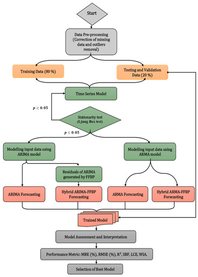
Figure 7.
The architecture of the proposed hybrid models is the Auto-Regressive Integrated Moving Average-Feed Forward back-propagation algorithm (ARIMA-FFBP) and Auto Regressive Moving Average-Feed Forward back-propagation algorithm (ARMA-FFBP).
- -
- Data pre-processing in section one (grey color) involves the collection of meteorological, computational, astronomical, and geographical data. These parameters require many corrections of missing data and outlier removal.
- -
- The application of multiple combinations of several input parameters in order to select the appropriate architecture executed in section two (gold color) was accomplished by splitting data into two steps, which are training data (80%), testing, and validation (20%) data.
- -
- The step of the training (green color) was operating the proposed methodologies. The input parameters were tested by using time series model stationarity (Ljung–Box test). After that, the data stationarity was implemented for ARIMA and ARMA models. In the case of the ARIMA model, that involves the residual generated by the FFBP model, which built the combined ARIMA and FFBP models.
- -
- The models were built and divided into simple (ARMA, ARIMA, and FFBP), and hybrid methods (hybrid ARMA-FFBP and hybrid ARIMA-FFBO models; orange color).
- -
- The obtained result (grey color) was evaluated and interpreted by using various statistical metrics in order to choose the best model, which presents the lowest value of MBE (%), RMSE (% Sd (%), AIC, and BIC and the highest values of R2, SBF, LCE, WIA.
2.5. Model Selection
According to the fundamental issues observed by modern data, the scientist has introduced meaningful conclusions for a complicated system utilizing data from a single determined parameter. Meanwhile, the most effective treatment of global solar radiation data involves the deployment of neural networks, either with data from each measurement or with data from several successive measurements. The management is describable as Equation (10),
where γ represents the neural network forecaster and i is the number of successive observations. Figure 8A–C above show that ACF and PACF can have on the auto-correlogram of the global solar radiation time series. Here the night hours have not considered during the simulations [44], and several measurements taken daily have been made.
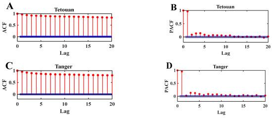
Figure 8.
(A,C) autocorrelation function (ACF) and (B,D) partial autocorrelation function (PACF) of the daily GSR from two cities.
The parameters of the ARIMA (p, d, q) and ARMA (p, q) models were determined by plotting The Autocorrelation Function (ACF) and the Partial Autocorrelation Function (PACF) for different lags (Lag). Figure 8A–D illustrate the daily global solar radiation data with a 95% confidence interval. According to the figure, the significant Lags in PACF are shown at Lag 7 for Tetouan city, and Lag 16 for Tangier city. Further in ACF, the Lag shows a geometric decrease at each Lag (i.e., 1, 2, 3, 4) and the order of the autoregressive term in the ARMA model for Tetouan and Tangier city is 10 and 16. Concerning the ARIMA (p, d, q) model, the order of the p and d terms is 2, 1 for Tetouan city, and 2, 2 for Tangier city. In addition, the use of the stationarity method (first and second differentiation for the ARIMA model) improves the prediction phenomenon, and the effectiveness of improvements in stationarity with the quality of the prediction would be discussed later in this study.
Table 3 and Table 4 compare the FFBP with the ARIMA and ARMA models, and deliver an example for optimization of the ARIMA and ARMA models with the parameters estimated from the two study sites. It is further considered that the prediction of the two techniques is relatively simple and eliminated the moving average order q (q = 0).

Table 3.
Estimation of ARMA model parameters for daily global solar radiation prediction for both cities.

Table 4.
Estimation of ARIMA model parameters for the prediction of daily global solar radiation of the two cities (Tetouan and Tangier).
In the models, the measurement data set has divided into three parts: a learning set (80%), a validation set (10%), and a test set (10%).
The weight (wij) adjustment is performed by the training set, and the validation set assures whether the error is within a certain range (this set is not adjusted weights directly, instead giving the optimal number of hidden layers or determining a breakpoint for the backscatter algorithm). Finally, the accuracy of the model on the test data facilitates the prediction performance of the model.
The hidden layer could be suggested even for preliminary analysis or modeling. Further, the application of more than one hidden layer has significantly increased the number of measurable variables. However, the improvement in the number of variables would reduce the training phase without increasing network performance. In this analysis, one hidden layer has been implemented, and identifying the correct number of neurons in the hidden layer is critical for effective implementation since it greatly improves neural network efficiency. If the hidden layer has included insufficient neurons, the neural network output could be degrading. On the other side, if the hidden layer has accompanied by excess neurons, it would increase the parameter complexity and the training data set could be over-adjusted. Therefore, the most appropriate approach to determining the correct number of neurons in the hidden layer is through experiments, such as adopting a trial-and-error procedure [45]. The analysis of the results below presents the daily global solar radiation prediction set using the FFBP model. The application of multiple architectures has been deployed to select the appropriate model with a low value of root mean square error (RMSE in%). In addition, the selection of input variables is carried out by the combination method. Table 5 shows the prediction result of different FFBP architectures with coefficients of variation for the two cities.

Table 5.
Daily GSR forecasting models with multiple FFBP network architecture.
The training and validation set along with the change in the number of neurons in the hidden layer are essential factors in selecting the appropriate architecture of the FFBP model. Specifically, the root means square error (RMSE) has functioned as a comparison tool to measure the accuracy of different selected models. Moreover, the low value of RMSE (%) and coefficient of variation indicate the efficiency of the FFBP model. According to the results, the appropriate architecture for models was chosen as twelve input parameters, two neurons in hidden layers, and one output (DGSR) for the two cities. The value of RMSE (%) and the coefficient of variation in Tetouan city are 0.489% and 0.426%, and the RMSE value (%) and the coefficient of variation for Tangier city are 0.406% and 0. 382%.
2.6. Performance Criterion
In this study, the important statistical error metric indexes mentioned in the literature were considered to evaluate the precision of the forecasting methods [7,46,47]. The performance of ARIMA and ANN models are validated in terms of root mean square error (RMSE), mean bias error (MBE), standard deviation (σ), and correlation coefficient (R2).
The root means square error (RMSE) is a commonly employed calculation of the variations between the forecasted values by a model or an equation and the experimental values. Further, the RMSE is widely used to compare the actual deviation between the predicted and the measured value, modeling, and regression analysis (Equation (11)):
The mean bias error measures the model’s average bias and determines further measures to fix the model. The average bias in forecasting is represented by Equation (12):
Equation (13) expresses the standard deviation, which is a function of the amount of attenuation in a set of values:
In Equation (14), the R2 defines the appropriate sequential match among measured and forecasted values and the writing:
The slope of the best-fit line (SBF) defines the appropriate sequential match among measured and forecasted values and can be expressed by Equation (15):
The Willmott’s index of agreement (WIA) defines the appropriate sequential match among measured and forecasted values and can be expressed by Equation (16):
The Legate’s coefficient of efficiency (LCE) defines the appropriate sequential match among measured and forecasted values and can be expressed by Equation (17):
where t(x) and a(x) are the i-th forecasted and measured values of daily GSR, () presents the average of measured values of daily GSR, and N is a number of experimental data.
Another criterion named the X2 Information Criterion (AIC of order two) and the X2 information criteria (BIC) are explained in Equations (18) and (19), which are computed for both ANN and ARIMA models:
where m is the number of input–output models and npar is the number of parameters to identify. Moreover, if the RMSE statistics should gradually improve with the more added parameters, the AIC and BIC statistics penalize the model with more parameters and therefore tend to give rise to more parsimonious models. In this case, the ratio of (m/npar) is less than 60, and the second-order AIC has been evaluated to measure the performance of the model.
3. Results and Discussion
This section deals with forecast ability via five techniques of the daily GSR in two different cities in Morocco. The first and second methods are purely autoregressive (ARMA and ARIMA), and the third approach is called FFBP, which has utilized a backpropagation algorithm and the combined methods. In order to assess the success of these techniques, numerous statistical metrics which are commonly used in the literature are discussed. The proposed methodologies are widely operated to forecast the daily global solar radiation (GSR) using the MATLAB environment. In Table 3, Table 4 and Table 5, the selected models could be defined as ARMA (10, 0, 0), ARMA (16, 0, 0), ARIMA (2, 1, 1), ARIMA (2, 2, 1), and FFBP (12, 2, 1), respectively, for Tetouan and Tangier cities.
Figure 9A–D show the comparisons of the daily GSR forecasted by the proposed ARIMA, ARMA, FFBP, hybrid ARMA-FFBP, hybrid ARIMA-FFBP, and measured data of the Tetouan site. The Figures present the error forecasting (EF) of each model, which shows the agreement relationship between the forecasted methodologies and measured data. Considering Figure 4A and Table 6 together, it appears clearly that the R2, WIA, SBF, and LCE of the selected ARMA (10.0.0) present a significant accuracy and vary between 0.8074 and 0.9939. In terms of BIC and AIC, the selected model presents the worst values forecasting after the ARIMA (2.1.0) model. The average value of the daily GSR forecasted by the ARMA (10.0.0) model is lower than the average daily GSR measured. In terms of error forecasting, it is seen that the selected model presents various observations with multiple error forecastings, like observation number 63 (EF = 1.878 kW·h/m2), 87 (EF = 2.378 kW·h/m2) 102 (EF = 2.818 kW·h/m2), and 263 (EF = 2.994 kW·h/m2), respectively.
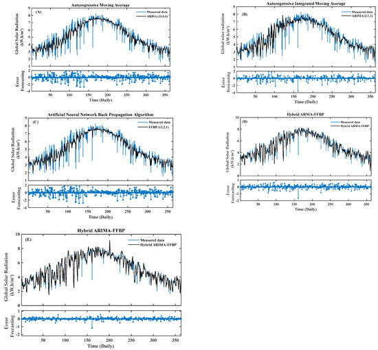
Figure 9.
(A–E) Comparison between predicted and measured values of daily global solar radiation from ARMA, FFBP, ARIMA, and hybrid models.

Table 6.
Statistical results of the FFBP, ARMA, ARIMA, and hybrid network models.
Figure 9B shows the daily GSR forecasted by the ARIMA (2.1.0) model and error forecasting. In addition, the forecasted ARIMA (2.1.0) is compared with the measured daily GSR for the Tetouan site. Considering the performance accuracy result presented in Table 6, it can be seen that the all-statistical metric indicates that the ARIMA (2.1.0) model forecast well through the lowest value of the MBE (0.0839%), RMSE (16.6421%), and Sd (12.6704%). In term of R2, the ARIMA (2.1.0) is 0.9628, which presents successful forecasting accuracy compared with the ARMA (10.0.0) model. The considering error forecasting of the ARIMA (2.1.0) model was seen in observation number 161 (3.542 kW·h/m2).
Figure 9C shows the daily GSR and EF of both forecasted FFBP (12.2.1) and measured data. By comparing the two previous models and the FFBP (12.2.1) model in terms of R2, the shown model gives the highest accuracy, which is estimated at 0.9890. The lowest value of the FFBP (12.2.1) in terms of the MBE, RMSE, BIC, and AIC is 0.817 kW·h/m2, 0.5119 kW·h/m2, 991.3442, and 890.6528, respectively. Unlike the ARMA (10.0.0) and ARIMA (2.1.0) models, the error forecasting of the significant FFBP (12.2.1) model is less in observation number 161(3.542 kW·h/m2) compared with ARIMA (2.1.0) and ARMA (10.0.0). It can be concluded that the FFBP (12.2.1) model performed better than the ARMA (10.0.0) and ARIMA (2.1.0) models.
Figure 9D shows the forecasted hybrid ARMA-FFBP model for the daily GSR, measured data, and error forecasting of the Tetouan site. Taking into account the advantage of a hybrid model, which can minimize the shortcomings of a single model, the shown hybrid ARMA-FFNB model is close to the measured data. In terms of R2, SBF, LCE, and WIA, the presented value of the hybrid model is 0.9890, 0.9148, 0.9580, and 0.9910, respectively. The R2 value is close to one, which indicates the good agreement between forecasted hybrid ARMA-FFBP and measured data. The other statistical metric of the hybrid ARMA-FFBP shows the lowest values compared with the three previous models. The error forecasting of the proposed hybrid ARMA-FFBP model shows significant and lower values than other models. Among the three previous models, it was seen that the hybrid ARMA-FFBP is the most suitable model to forecast the daily GSR compared with ARMA (10.0.0), ARIMA (2.1.0), and FFBP (12.2.1) models.
Figure 9E shows the forecasted daily GSR generated by the hybrid ARIMA-FFBP model, the measured data, and the error forecasting of the Tetouan site. Among all models, the hybrid ARIMA-FFBP is the most successful model, which is very close to the measured daily GSR. In terms of R2, the shown hybrid ARIMA-FFBP is approximately higher by about 0.41% on the hybrid ARMA- FFBP model, 0. 53% on the FFBP (12.2.1) model, 4.59% on the ARMA (10.0.0) model and around 3.03% on ARIMA (2.1.0) model. The computed MBE (%), RMSE (%) Sd (%), SBF, LCE, WIA, BIC, and AIC showed a very close forecasting success compared with FFBP (12.2.1) and hybrid ARMA-FFBP models. The Hybrid ARMA-FFBP model is close to the hybrid ARIMA-FFBP model, particularly in R2 (%). In term of error forecasting, the proposed hybrid ARIMA-FFBP can be recognized as “the very most suitable model forecasting”, which present the lowest value of statistical performance and the highest values of R2, SPE, LCE, and WIA. Likewise, particularly in the previous observation number 161, the presented error forecasting of the hybrid ARIMA-FFBP was seen to be very low.
Figure 10A–D shows the comparisons of the daily GSR forecasted by the proposed ARIMA, ARMA, FFBP, hybrid ARMA-FFBP, hybrid ARIMA-FFBP, and measured data of the Tangier site. The Figures present the error forecasting (EF) of each model, which shows the agreement relationship between the forecasted methodologies and measured data. The study location presents satisfactory results in terms of statistical metrics in the same way as the previous one. The Tangier site is among the Mediterranean regions with good prediction results selected in this study. In this regard, it has been seen from the forecasted results and error depicted in Figure 5. Various observation numbers seen from the forecasted daily GSR have maximal and minimal error forecasting. The presented result led to increasing and decreasing the total forecast error of the selected study location. The reason why the Tangier site is less expected than the Tetouan site. The ARMA (16.0.0) has been the worst forecasted model in terms of R2, SPE, LCE, and WIA for the Tangier site. The range value of the selected model is between 0.8074 and 0.9601. Compared with the Tetouan site, the ARMA (16.0.0) model performed better than the ARMA (10.0.0) model.
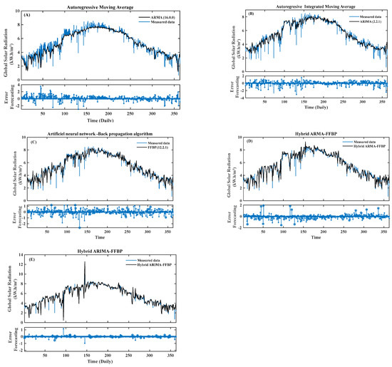
Figure 10.
(A–E) Comparison between predicted and measured values of daily global solar radiation from ARMA, FFBP, ARIMA, and hybrid models.
Figure 10B shows the daily GSR forecasted by ARIMA (2.2.0) model compared with the measured data. In terms of MBE (%), RMSE (%), Sd (%), AIC, and BIC, the proposed model increases the forecast accuracy compared with ARMA (16.0.0) model. The error forecasting in this model is less than ARMA (16.0.0) model. Particularly, in observation numbers 73 (1.98 kW·h/m2), 88 (3.638 kW·h/m2), 89 (2.95 kW·h/m2) 128 (5.368 kW·h/m2), 131 (3.882 kW·h/m2), and 360 (0.6491 kW·h/m2). In terms of MBE, the selected model is the only one that has the lowest value (0.0042 kW·h/m2) compared to the other models. It can be concluded that the ARIMA (2.2.0) exceeds the ARMA (16.0.0) model and present a significant agreement between the forecasted daily GSR and measured data.
Figure 10C shows the comparisons of the forecasted daily GSR generated by the FFBP (12.2.1) method and measured data for the Tangier site. The error forecast is depicted in the same figure, which presents the forecast improvement FFBP (12.2.1), and the performance accuracy between measured data. As seen from Table 6, in term of R2, the selected model rank third after the combined models. The lowest value of the FFBP (12.2.1) is by about 0.03092 kW·h/m2 for MBE, 0.0517% for MBE (%), and 0.79265 (%) for Sd (%) respectively. The highest value of WIA is about 0.9891 and is nearly close to 1. As a result, the selected FFBP (12.2.1) exceeds the ARIMA (2.2.0) and ARMA (16.0.0) models and illustrates a successful forecast of the daily GSR.
Figure 10D shows the daily GSR forecasted by the hybrid ARMA-FFBP model and error forecasting. In addition, the forecasted combined model is compared with the measured daily GSR for the Tangier site. Considering the depicted Figure 5 and Table 6 together, it appears clearly that the hybrid ARMA-FFBP presents the highest statistical metric indicator compared with the previous model for the selected study location. In addition, the combined ARMA-FFPB is close to FFBP (12.2.1) in terms of R2, Sd (%), and Sd. Unlike the ARMA (16.0.0) and ARIMA (2.2.0) models, the error forecasting of the significant hybrid ARMA-FFBP model is less in observation numbers 73 (1.98 kW·h/m2), 88 (3.638 kW·h/m2), 89 (2.95 kW·h/m2) 128 (5.368 kW·h/m2), 131 (3.882 kW·h/m2), and 360 (0.6491 kW·h/m2).
Figure 10E shows the forecasted daily GSR implemented by combined ARIMA-FFBP and compared with those measured data for the Tangier site. Among the four previous models, the hybrid ARIMA-FFBP is the most successful model, which presents the lowest values of MBE (%), RMSE (%), Sd (%), AIC, and BIC, and the highest value of R2, SPE, LCE, and WIA. In terms of R2, the shown hybrid ARIMA-FFBP is approximately higher by about 1.57% on the ARMA (16.0.0) model, 3% on the ARIMA (2.2.0) model, 0.67% on the FFBP (12.2.1) model, and around 0.13% on the hybrid ARMA-FFBP (2.1.0) model. All computed statistical performance metrics showed a very close forecasting success compared with the FFBP (12.2.1) and hybrid ARMA-FFBP models. In terms of error forecasting, the proposed hybrid ARIMA-FFBP can be recognized as “the very most suitable model forecasting”. Likewise, in the previous observation number, the presented error forecasting of the hybrid ARIMA-FFBP was seen to be very low.
The Taylor diagram has been utilized as a comparison tool revealing the accuracies of different selected models (forecasted and measured data). Moreover, this diagram combines the correlation coefficient (R2), the root means square error (RMSE), and the standard deviation (Sd) in a polar (two-dimensional) diagram. The main objective of this illustration is to closely inspect the forecasted results and the measured data on a particular day. Figure 11 and Figure 12 compare the performance of the most appropriate inputs, and graphs based on the statistical error metric. The figures illustrate the accuracies of the 16 relevant models, which have relatively lower errors in terms of standard deviation (Sd) and RMSE (value between 0.1 and 0.8 kWh/m2). In addition, the, highest value of R2 (99.31%) presents the accuracy relationship between the measured and predicted values.
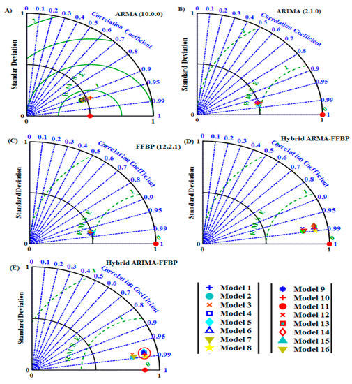
Figure 11.
Taylor diagram of several (A) ARMA, (B) ARIMA, (C) FFBP, and (D,E) hybrid models of Tetouan city.
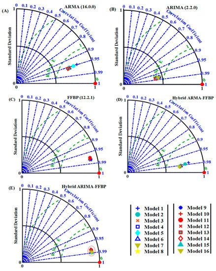
Figure 12.
Taylor diagram of several (A) ARMA, (B) ARIMA, (C) FFBP, and (D,E) hybrid models of Tangier city.
Figure 11 illustrates the Taylor diagram for the Tetouan site, in which statistics for the forecasted ARMA (10.0.0), ARIMA (2.1.0), FFBP (12.2.1), hybrid ARMA-FFBP, and hybrid ARIMA-FFBP models (each model contains 16 appropriate models to select the performed one) were computed. Each appropriate model appearing in the diagram quantifies how the forecasted models matched measured daily GSR. It is seen from the figure that the centered RMSE is related to the distance from the reference point (the horizontal axis is considered as observed data). As a result, the forecasted ARMA (10.0.0) and ARIMA (2.1.0) revealed the highest RMSE and the lowest value of R2, which is varying between 16.6421~15.6709 and 0.9472~0.9628, respectively. This model is less than the forecasted FFBP (12.2.1) model and revealed the optimum RMSE (0.5119%) and Sd (9.9852%). The forecasted combined hybrid ARMA-FFBP and hybrid-FFBP models resulted in the lowest value of RMSE than the simple models.
The Taylor diagram for the Tangier site shown in Figure 12 is generated by five models, which contain 16 appropriate models. It appears from the figure that the forecasted FFBP (12.2.1), hybrid ARMA-FFBP, and ARIMA-FFBP models proved the appropriate match with the measured daily GSR. The hybrid ARIMA-FFBP model had the highest values in terms of R2 and the lowest value in terms of RMSE compared with previous models. In this case study, the Taylor correlation increased by about 10% to 15% compared with the Tetouan site.
The regression plot of the forecasted daily GSR generated by the most five appropriate models for the Tetouan and Tangier sites is given in Figure 13A,B. As seen from the figures, the error estimated between the forecasted daily GSR and measured data have a wide dispersion of the ARMA (10.0.0), ARIMA (2.1.0), ARMA (16.0.0), and ARIMA (2.2.0) models for Tetouan and Tangier site, respectively. The dispersion of the FFBP (12.2.1) model is smaller than the other two previous models. The dispersion of the combined models is smaller and less than the FFBP (12.2.1) model. The accuracy between the forecasted and measured data in the hybrid ARIMA-FFBP method is improved. It is observed that all data sets are correctly fitted to the corresponding line, which verifies the hybrid ARIMA-FFBP is more accurate compared to other methods. In addition, the correlation coefficient (R2) values of the best model for the Tetouan and Tangier sites is close to 1, which explains the good relationship between the forecasted and measured data.
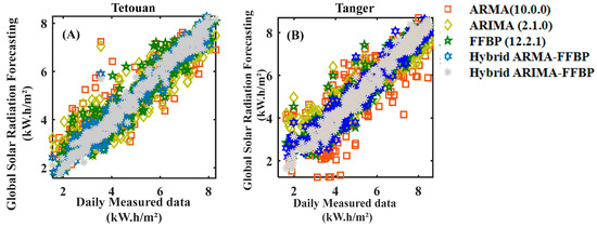
Figure 13.
(A,B) Correlation coefficient (R2) of daily GSR vs. measured data of best five models (regression plot).
Table 6 gives the numerical values of the adopted methodologies by using the computed statistical metric in order to select the best model, which is at present the optimal value. The correlation coefficient (R2) of the forecasted ARIMA, ARMA, FFBP, and hybrid models varies between 0.9472% and 0.9931% depending on the study location and the trained methods. The range value of the slope of the best-fit line (SPE) varies between 0.8435 and 0.9296. The range value of the legate’s coefficient of efficiency (LCE) is 0.8954, 0.9696 and the range value of Willmott’s index of agreement (WIA) is 0.9491 and 0.9945. These results show that the hybrid ARIMA-FFBP is more reliable in the forecasting of the daily GSR for the Tetouan and Tangier sites. In this context, the obtained performance will be compared and discussed by considering Table 6 as the reference. Further, the results obtained from the hybrid ARIMA-FFBP model compared with single and combined models have exposed the highest correlation coefficient of 0.9901% for Tetouan city and 0.9831% for Tangier city. In addition, the values of MBE (%), RMSE (%), Sd (%), Akaike information criterion (AIC), and Bayesian information criterion (BIC) for both cities are 0.0297 (%), 0.02101 (%), 9.6917 (%), 9.06742 (%), 8.67911 (%), 6.87613 (%), 792.8625, 765.091 and 756.3418, 504.816, respectively. Eventually, the results have defined that the hybrid ARIMA-FFBP model is more accurate and suitable compared with the other methods to predict the daily global solar radiation for any location with the same weather conditions.
In several investigations, the hybrid ARIMA-FFBP and hybrid ARMA-FFBP models were compared to deep learning models for solar radiation. A study, for example, compared artificial intelligence (AI) methods for solar radiation forecast or estimation, including empirical, statistical, physical, and machine learning models [25]. Another study introduced a new hybrid strategy based on deep learning approaches for Global Solar Radiation (GSR) prediction problems [48]. In addition, one study constructed and analyzed two innovative hybrid neural network models for solar irradiance forecasting [49], and another examined the effects of various classic long short-term memory (LSTM) models on hour-ahead solar irradiance forecasting [50]. Finally, a study demonstrated that using input parameters in this hybrid model for daily GSR forecast proves the performance accuracy compared to the previous models.
4. Conclusions
This paper has evaluated and compared the forecasting of the daily global solar radiation in two cities by five approaches such as FFBP, ARIMA, ARMA, hybrid ARMA-FFBP, and hybrid ARIMA-FFBP, which were modeled in the MATLAB simulation platform. A different combination of input data was used to achieve our proposed methodologies in terms of statistical metrics. Further, the forecasting accuracy of the FFBP model in various applications and the analysis capability time series of the ARIMA and ARMA models were considered. Moreover, the solar radiation intensity, according to the climatic conditions and geographical coordinates in the two cities, was evaluated by their measured daily GSR dataset.
The hybrid ARIMA-FFBP model obtained the highest correlation coefficient of 0.9901% for Tetouan city and 0.9831% for Tangier city once compared to single and combined models. MBE (%), RMSE (%), Sd (%), Akaike information criterion (AIC), and Bayesian information criterion (BIC) values for both cities are 0.0297 (%), 0.02101 (%), 9.6917 (%), 9.06742 (%), 8.67911 (%), 6.87613 (%), 792.8625, 765.091, and 756.3418, 504.816, respectively. Furthermore, the results reveal that the hybrid ARIMA-FFBP model has been considered an appropriate forecasting tool to predict the daily global solar radiation, which exceeds the hybrid ARMA-FFBP and the other models. This method could be deployed further for modeling different areas in the country for long-term forecasting. Notably, the most appropriate model has corresponded to the lowest value of statistical performance indicators. For instance, the hybrid ARIMA-FFBP model reaches low values compared to the hybrid ARMA-FFBP and simple models. Ultimately, the results verify that the hybrid ARIMA-FFBP model is highly accurate in predicting the daily global solar radiation and could further be substituted for other locations under similar weather conditions in the future.
Author Contributions
Conceptualization, B.B. and M.L.; methodology, B.B.; software, B.B.; validation, B.B., M.L. and M.M.; formal analysis, A.E.B.; investigation, B.B.; resources, B.B.; data curation, B.B.; writing—original draft preparation, B.B.; visualization, M.L.; supervision, M.M.; project administration, B.B.; funding acquisition, A.E.B. All authors have read and agreed to the published version of the manuscript.
Funding
This research received no external funding.
Data Availability Statement
The data are available in the request for the first author.
Conflicts of Interest
The authors declare no conflict of interest.
References
- Suresh, M.; Meenakumari, R.; Panchal, H.; El Agouz, E.S.; Israr, M. An enhanced multiobjective particle swarm optimization algorithm for optimum utilization of hybrid renewable energy systems. Int. J. Ambient Energy 2020, 43, 2540–2548. [Google Scholar] [CrossRef]
- Ma, T.; Yang, H.; Lu, L.; Peng, J. Optimal design of an autonomous solar–wind-pumped storage power supply system. Appl. Energy 2015, 160, 728–736. [Google Scholar] [CrossRef]
- Belmahdi, B.; El Bouardi, A. Simulation and optimization of microgrid distributed generation: A case study of university abdelmalek essaâdi in Morocco. Procedia Manuf. 2020, 46, 746–753. [Google Scholar] [CrossRef]
- Mellit, A.; Pavan, A.M. A 24-h forecast of solar irradiance using artificial neural network: Application for performance prediction of a grid-connected PV plant at Trieste, Italy. Sol. Energy 2010, 84, 807–821. [Google Scholar] [CrossRef]
- Belmahdi, B.; El Bouardi, A. Solar potential assessment using PVsyst software in the northern zone of Morocco. Procedia Manuf. 2020, 46, 738–745. [Google Scholar] [CrossRef]
- Lan, H.; Zhang, C.; Hong, Y.-Y.; He, Y.; Wen, S. Day-ahead spatiotemporal solar irradiation forecasting using frequency-based hybrid principal component analysis and neural network. Appl. Energy 2019, 247, 389–402. [Google Scholar] [CrossRef]
- Louzazni, M.; Mosalam, H.; Khouya, A. A non-linear auto-regressive exogenous method to forecast the photovoltaic power output. Sustain. Energy Technol. Assess. 2020, 38, 100670. [Google Scholar] [CrossRef]
- Belmahdi, B.; Louzazni, M.; El Bouardi, A. A hybrid ARIMA–ANN method to forecast daily global solar radiation in three different cities in Morocco. Eur. Phys. J. Plus 2020, 135, 925. [Google Scholar] [CrossRef]
- Pereira, S.; Canhoto, P.; Salgado, R.; Costa, M.J. Development of an ANN based corrective algorithm of the operational ECMWF global horizontal irradiation forecasts. Sol. Energy 2019, 185, 387–405. [Google Scholar] [CrossRef]
- Koca, A.; Oztop, H.F.; Varol, Y.; Koca, G.O. Estimation of solar radiation using artificial neural networks with different input parameters for Mediterranean region of Anatolia in Turkey. Expert Syst. Appl. 2011, 38, 8756–8762. [Google Scholar] [CrossRef]
- Büyükşahin, Ü.Ç.; Ertekin, Ş. Improving forecasting accuracy of time series data using a new ARIMA-ANN hybrid method and empirical mode decomposition. Neurocomputing 2019, 361, 151–163. [Google Scholar] [CrossRef]
- Kazantzidis, A.; Nikitidou, E.; Salamalikis, V.; Tzoumanikas, P.; Zagouras, A. New challenges in solar energy resource and forecasting in Greece. Int. J. Sustain. Energy 2018, 37, 428–435. [Google Scholar] [CrossRef]
- Liu, Y.; Qin, H.; Zhang, Z.; Pei, S.; Wang, C.; Yu, X.; Jiang, Z.; Zhou, J. Ensemble spatiotemporal forecasting of solar irradiation using variational Bayesian convolutional gate recurrent unit network. Appl. Energy 2019, 253, 113596. [Google Scholar] [CrossRef]
- Fouilloy, A.; Voyant, C.; Notton, G.; Motte, F.; Paoli, C.; Nivet, M.L.; Guillot, E.; Duchaud, J.L. Solar irradiation prediction with machine learning: Forecasting models selection method depending on weather variability. Energy 2018, 165, 620–629. [Google Scholar] [CrossRef]
- Belmahdi, B.; Louzazni, M.; Akour, M.; Cotfas, D.T.; Cotfas, P.A.; El Bouardi, A. Long-term global solar radiation prediction in 25 cities in morocco using the FFNN-BP method. Front. Energy Res. 2021, 9, 733842. [Google Scholar] [CrossRef]
- Belmahdi, B.; Louzazni, M.; El Bouardi, A. Comparative optimization of global solar radiation forecasting using machine learning and time series models. Environ. Sci. Pollut. Res. 2021, 29, 14871–14888. [Google Scholar] [CrossRef]
- Mellit, A. Artificial Intelligence technique for modelling and forecasting of solar radiation data: A review. Int. J. Artif. Intell. Soft Comput. 2008, 1, 52–76. [Google Scholar] [CrossRef]
- López, G.; Batlles, F.J.; Tovar-Pescador, J. Selection of input parameters to model direct solar irradiance by using artificial neural networks. Energy 2005, 30, 1675–1684. [Google Scholar] [CrossRef]
- Lampinen, J.; Vehtari, A. Bayesian approach for neural networks—Review and case studies. Neural Netw. 2001, 14, 257–274. [Google Scholar] [CrossRef]
- Penny, W.D.; Roberts, S.J. Bayesian neural networks for classification: How useful is the evidence framework? Neural Netw. 1999, 12, 877–892. [Google Scholar] [CrossRef]
- Benvenuto, D.; Giovanetti, M.; Vassallo, L.; Angeletti, S.; Ciccozzi, M. Application of the ARIMA model on the COVID-2019 epidemic dataset. Data Brief 2020, 29, 105340. [Google Scholar] [CrossRef]
- Jamil, R. Hydroelectricity consumption forecast for Pakistan using ARIMA modeling and supply-demand analysis for the year 2030. Renew. Energy 2020, 154, 1–10. [Google Scholar] [CrossRef]
- Wang, W.; Chau, K.; Xu, D.; Chen, X.-Y. Improving forecasting accuracy of annual runoff time series using ARIMA based on EEMD decomposition. Water Resour. Manag. 2015, 29, 2655–2675. [Google Scholar] [CrossRef]
- Gibrilla, A.; Anornu, G.; Adomako, D. Trend analysis and ARIMA modelling of recent groundwater levels in the White Volta River basin of Ghana. Groundw. Sustain. Dev. 2018, 6, 150–163. [Google Scholar] [CrossRef]
- Bamisile, O.; Oluwasanmi, A.; Ejiyi, C.; Yimen, N.; Obiora, S.; Huang, Q. Comparison of machine learning and deep learning algorithms for hourly global/diffuse solar radiation predictions. Int. J. Energy Res. 2022, 46, 10052–10073. [Google Scholar] [CrossRef]
- Bamisile, O.; Cai, D.; Oluwasanmi, A.; Ejiyi, C.; Ukwuoma, C.C.; Ojo, O.; Mukhtar, M.; Huang, Q. Comprehensive assessment, review, and comparison of AI models for solar irradiance prediction based on different time/estimation intervals. Sci. Rep. 2022, 12, 9644. [Google Scholar] [CrossRef]
- Huang, L.; Kang, J.; Wan, M.; Fang, L.; Zhang, C.; Zeng, Z. Solar radiation prediction using different machine learning algorithms and implications for extreme climate events. Front. Earth Sci. 2021, 9, 596860. [Google Scholar] [CrossRef]
- Atique, S.; Noureen, S.; Roy, V.; Subburaj, V.; Bayne, S.; MacFie, J. Forecasting of total daily solar energy generation using ARIMA: A case study. In Proceedings of the 2019 IEEE 9th Annual Computing and Communication Workshop and Conference, CCWC 2019, Las Vegas, NV, USA, 7–9 January 2019; pp. 114–119. [Google Scholar] [CrossRef]
- Shams, M.B.; Haji, S.; Salman, A.; Abdali, H.; Alsaffar, A. Time series analysis of Bahrain’s first hybrid renewable energy system. Energy 2016, 103, 1–15. [Google Scholar] [CrossRef]
- Hussain, S.; Al Alili, A. Day ahead hourly forecast of solar irradiance for Abu Dhabi, UAE. In Proceedings of the 2016 4th IEEE International Conference on Smart Energy Grid Engineering, SEGE 2016, Oshawa, ON, Canada, 21–24 August 2016; pp. 68–71. [Google Scholar] [CrossRef]
- Gairaa, K.; Khellaf, A.; Messlem, Y.; Chellali, F. Estimation of the daily global solar radiation based on Box-Jenkins and ANN models: A combined approach. Renew. Sustain. Energy Rev. 2016, 57, 238–249. [Google Scholar] [CrossRef]
- Hassan, J. ARIMA and regression models for prediction of daily and monthly clearness index. Renew. Energy 2014, 68, 421–427. [Google Scholar] [CrossRef]
- Sulaiman, M.Y.; Wahab, M.A.; Sulaiman, Z.A. Analysis of residuals in daily solar radiation time series. Renew. Energy 1997, 11, 97–105. [Google Scholar] [CrossRef]
- Wang, Z.; Wang, F.; Su, S. Solar irradiance short-term prediction model based on BP neural network. Energy Procedia 2011, 12, 488–494. [Google Scholar] [CrossRef]
- Vu, K.M. The ARIMA and VARIMA Time Series: Their Modelings, Analyses and Applications; AuLac Technologies: Ottawa, ON, Canada, 2007. [Google Scholar]
- Chatfield, C.; Xing, H. The Analysis of Time Series: An Introduction with R, 7th ed.; CRC Press: Boca Raton, FL, USA; Taylor & Francis Group: Abingdon, UK, 2019. [Google Scholar]
- Tsay, R.S. Analysis of Financial Time Series; Wiley: Hoboken, NJ, USA, 2010. [Google Scholar]
- Sansa, I.; Boussaada, Z.; Bellaaj, N.M. Solar radiation prediction using a novel hybrid model of ARMA and NARX. Energies 2021, 14, 6920. [Google Scholar] [CrossRef]
- Shadab, A.; Said, S.; Ahmad, S. Box–Jenkins multiplicative ARIMA modeling for prediction of solar radiation: A case study. Int. J. Energy Water Resour. 2019, 3, 305–318. [Google Scholar] [CrossRef]
- Akaike, H. Information Theory and an Extension of the Maximum Likelihood Principle; Springer: New York, NY, USA, 1998; pp. 199–213. [Google Scholar] [CrossRef]
- Belmahdi, B.; Louzazni, M.; El Bouardi, A. One month-ahead forecasting of mean daily global solar radiation using time series models. Optik 2020, 219, 165207. [Google Scholar] [CrossRef]
- McQuarrie, A.D.R.; Tsai, C.-L. Regression and Time Series Model Selection; World Scientific: Singapore, 1998. [Google Scholar]
- Somvanshi, V.K.; Pandey, O.P.; Agrawal, P.K.; Kalanker, N.; Prakash, M.R.; Chand, R. Modelling and prediction of rainfall using artificial neural network and ARIMA techniques. J. Ind. Geophys. Union 2006, 10, 141–151. [Google Scholar]
- Sudheer, K.P.; Gosain, A.K.; Ramasastri, K.S. A data-driven algorithm for constructing artificial neural network rainfall-runoff models. Hydrol. Process. 2002, 16, 1325–1330. [Google Scholar] [CrossRef]
- Hammerstrom, D. Working with neural networks. IEEE Spectr 1993, 30, 46–53. [Google Scholar] [CrossRef]
- Louzazni, M.; Khouya, A.; Amechnoue, K.; Mussetta, M.; Crăciunescu, A. Comparison and evaluation of statistical criteria in the solar cell and photovoltaic module parameters’ extraction. Int. J. Ambient Energy 2020, 41, 1482–1492. [Google Scholar] [CrossRef]
- Al-Dahidi, S.; Ayadi, O.; Adeeb, J.; Louzazni, M. Assessment of artificial neural networks learning algorithms and training datasets for solar photovoltaic power production prediction. Front. Energy Res. 2019, 7, 130. [Google Scholar] [CrossRef]
- Jaihuni, M.; Basak, J.K.; Khan, F.; Okyere, F.G.; Arulmozhi, E.; Bhujel, A.; Park, J.; Hyun, L.D.; Kim, H.T. A partially amended hybrid bi-gru—ARIMA model (PAHM) for predicting solar irradiance in short and very-short terms. Energies 2020, 13, 435. [Google Scholar] [CrossRef]
- Mukhtar, M.; Oluwasanmi, A.; Yimen, N.; Qinxiu, Z.; Ukwuoma, C.C.; Ezurike, B.; Bamisile, O. Development and comparison of two novel hybrid neural network models for hourly solar radiation prediction. Appl. Sci. 2022, 12, 1435. [Google Scholar] [CrossRef]
- Huang, X.; Zhang, C.; Li, Q.; Tai, Y.; Gao, B.; Shi, J. A Comparison of hour-ahead solar irradiance forecasting models based on LSTM network. Math. Probl. Eng. 2020, 2020, 4251517. [Google Scholar] [CrossRef]
Disclaimer/Publisher’s Note: The statements, opinions and data contained in all publications are solely those of the individual author(s) and contributor(s) and not of MDPI and/or the editor(s). MDPI and/or the editor(s) disclaim responsibility for any injury to people or property resulting from any ideas, methods, instructions or products referred to in the content. |
© 2023 by the authors. Licensee MDPI, Basel, Switzerland. This article is an open access article distributed under the terms and conditions of the Creative Commons Attribution (CC BY) license (https://creativecommons.org/licenses/by/4.0/).