Article

Load Forecasting in an Office Building with Different Data Structure and Learning Parameters

1
GECAD—Research Group on Intelligent Engineering and Computing for Advanced Innovation and Development, Rua DR, Antonio Bernardino de Almeida 431, 4200-072 Porto, Portugal
2
Polytechnic of Porto, Rua DR, Antonio Bernardino de Almeida 431, 4200-072 Porto, Portugal
*
Author to whom correspondence should be addressed.
Forecasting 2021, 3(1), 242-255; https://doi.org/10.3390/forecast3010015
Submission received: 30 January 2021 / Revised: 16 March 2021 / Accepted: 17 March 2021 / Published: 20 March 2021
(This article belongs to the Special Issue Feature Papers of Forecasting 2021)

Abstract

:
Energy efficiency topics have been covered by several energy management approaches in the literature, including participation in demand response programs where the consumers provide load reduction upon request or price signals. In such approaches, it is very important to know in advance the electricity consumption for the future to adequately perform the energy management. In the present paper, a load forecasting service designed for office buildings is implemented. In the building, using several available sensors, different learning parameters and structures are tested for artificial neural networks and the K-nearest neighbor algorithm. Deep focus is given to the individual period errors. In the case study, the forecasting of one week of electricity consumption is tested. It has been concluded that it is impossible to identify a single combination of learning parameters as different parts of the day have different consumption patterns.

1. Introduction

Energy consumption forecast is very important in the context of energy consumption management towards improved energy efficiency. The forecast’s accuracy may be improved based on retraining with a fixed size of training, discarding older information while retaining new information. The selection of sensors from smart technologies is another aspect that provides more training data that are expected to decrease the forecast errors [1].
The electricity markets face possible generation costs caused by environmental issues [2,3]. Smart grids are implemented in many of these markets, supporting efficient energy use [4]. Solutions involving smart grids consist of an adequate consumer schedule aimed to reduce the electricity consumption in particular periods [5]. These solutions are contextualized when markets launch demand response programs to make the consumption schedule adequate to reduce electricity costs interpreted by peaks [6].
Smart buildings play an important role in the electricity sector to satisfy occupants’ electric needs and exploit operational flexibilities. Therefore, the launch of model optimization evidences the need to control the microgrids’ power flows [7]. To deal with the situation, it requires solutions from demand response programs, reducing the energy costs using the smart grid opportunities to readapt the consumption to play an important role in load management and energy efficiency [8].
The optimization of electrical energy is possible with data monitored from a measurement system that captures real-time data and automatic forecasting [9,10]. With regard to forecasting, several machine learning algorithms can be used [11,12,13,14]. An artificial neural network (ANN) is described by layers containing neurons with weighted connections starting in an input layer, at least one hidden layer, and an output layer [15]. An alternative technique, K-nearest neighbor (KNN), performs data searches and associations in a large resource space with non-linear mapping support [16].
Various types of time-scaled forecast data may be evidenced in the field of energy, with Short Time Load Forecasting (STLF) being a good option. ANN is recommended for many short-term applications, including the prediction of daily peaks by using the training data with past data framed on past years [17]. KNN is suggested for both classification and regression tasks, and in the suggested approach, it is used for regression problems that involve energy predictions. The reduction of data complexity is a relevant aspect evidenced in the algorithm, possible with the nearest neighbors’ readaptation to several subsets of data [18]. An even more innovative algorithm is suggested in [19] featuring a KNN-ANN model that uses the K-nearest neighbors process while adding a backpropagation function known to be a particular aspect of an artificial neural network (ANN). The application of the KNN-ANN model is suggested for a stock price prediction problem. The NPower Forecasting Challenge, taken in the year 2015 edition evidenced in [20], challenges the participants to perform daily energy predictions of a customer group. Several algorithms, including artificial neural network and Random Forest, are suggested. In another study, students’ classification in algorithms like artificial neural network and Support Vector Machines is analyzed and their limitations are studied [21].
A research area of high interest is the energy efficiency of buildings—more specifically, the power distribution network that connects the equipment to end-users. The energy efficiency is highlighted on several worldwide applications including Supervisory Control And Data Acquisition (SCADA) and IoT systems [22]. These technologies allow the monitoring and management of consumption data on all the types of building from residential to commercial level. Thess data are relevant for the forecasting of data in the field of energy that are associated with electricity markets and policy formulations [23].
The forecasting of energy consumption with daily profile data usually improves the financial profit of consumers considering the monthly electricity bills reducing the peaks of energy detected in particular periods. The accuracy of energy forecasting algorithms depends on infrastructure and planning [24]. There are three ways to model an energy forecasting system mentioned in [25], including physics-based, data-driven, and hybrid models. While pros and cons are in question, the data-driven method has been proven as the best option for merging buildings in the smart grids. An additional factor that may improve the forecast reliability is to use sensor data that performs different measures according to each device according to smart meters [26,27]. The validation of forecasting models is another factor that should be taken into account in several smart buildings [28]. Real-time automatic energy forecasts with access to electric energy are recommended to be performed with data monitored in a building to achieve energy management optimization [29]. In [30], the component estimation technique is used for electricity consumption forecasts; historic consumption data were used. In [31], the impact of data quality in the electricity consumption forecast is discussed. The main focus is given to the dataset cleaning.
This paper provides a methodology to improve electricity consumption forecasting accuracy with sensor data measured by different devices, including presence, temperature, consumption, and humidity. The forecasting algorithms, namely ANN [32] and KNN [33], are implemented as a service and are the recommended options for the decision-making approaches to be used in the present paper. The innovative scientific aspect relies on the specific manipulations of data to overcome anomalies in data, including missing and excess occurrences. Second, the systematic analysis of different learning parameters is implemented to define the most relevant parameters in different periods of the day. This major aspect is usually treated in the literature by analyzing overall average forecasting errors without looking in detail at particular periods [34]. This aspect refers to a limitation in the recent literature, including the one published by the authors of the present paper in [1]. The forecasts are done for intervals (referred to as periods) of 5 min.
After this introduction, the proposed method is explained in Section 2, describing what is done at each stage. Proceeding to Section 3, the results of using the method are presented. The discussion is made in Section 4, and the main conclusions are presented in Section 5.

2. Materials and Methods

This section illustrates and explains the different phases of a method. The parameterization definition, the data reduction, the training and forecasting tasks, and the error calculation are parts of the tasks presented in Figure 1. The presented method is very important to support a building’s participation, namely an office building, in demand response programs [35]. Addressing consumer comfort, a SCADA system can make autonomous decisions for participation in demand response programs issued by the distribution network operator [36].
The innovative aspect of the present method is highlighted in green in Figure 1. As can be seen in the green arrow, the forecasting provides feedback to the training service regarding the accuracy of different learning parameters in different periods of the day. The test service is adapted to accommodate the fact that different periods of the day are related to different consumption patterns, so the test service must be run for each period. Different time frames are considered in the “Test service for different periods”, namely: weekly Symmetric Mean Absolute Percentage Error (SMAPE) accuracy; daily SMAPE accuracy; period of day SMAPE accuracy; specific period accuracy. SMAPE is defined in Equation (3). The periods in a day for SMAPE in this paper are considered to be three periods: 00:00 to 08:00; 08:00 to 17:00; and 17:00 to 24:00.
The tuning process performs parametrization of data required for later use on forecasting tasks with the support of analysis, studies, optimizations, and data manipulations. Two main aspects describe this process. The first one evaluates the data content analyzing the best possible forecasting technique that should provide better results in that specific situation. The second one performs data transformations to the initial dataset reducing the original version of data to a more accurate version fed by the forecasting technique that should provide more accurate forecasts. There is a balance between the completion and simplicity of data to avoid wrong interpretations. Therefore, data structure and reliability are two main aspects to improve the accuracy of the algorithm.
The real-time data consist of all monitored and persistent data that the building technologies track in the system more concretely with consumption and sensors data. The correlation process has the goal of analyzing which sensors are more associated with consumption. Both the tasks of providing a sample and the correlation study influence the participation towards reducing the dataset.
Despite reducing the dataset to the entire historic series, the same rules apply for real-time data. The forecasting methodology studies which technique is better for the sampling of data. Both the reduced version of the dataset and the forecasting method are sent to the training service.
The cleaning operation makes data more accurate for further use on forecasting tasks. It goes through several phases, starting with reorganizing all data in a unique spreadsheet with data split into several fields, including year, month, day of the month, days of the week, hours, and minutes. The criterion applied for missing information is to make sequential copies of previous records.
Outliers treatments are applied to detect erroneous readings made by technology devices. The outlier’s detection occurs with the support of the mean and standard deviation operations, as seen in Equations (1) and (2). The conditions implicit in the outlier’s detection with the support of the mean and standard deviation are presented in Equation (3), suggesting scenarios where a point is outside of an interval between two values: the average minus or plus of a product between the error factor and the standard deviation. In the present paper, consumptions above 4800 W or below 300 W are considered outliers. These values have been established according to the authors’ knowledge about building consumption.
A =   t = n F n P ( t ) F
  • A—average consumption in F;
  • n—current moment;
  • P—consumption;
  • t—index of time;
  • F—frame (time interval) used for calculation.
S = 1 F × t = n F n ( P ( t ) A ) 2
  • S—standard deviation consumption in F;
  • F—frame used for calculation.
The service ends by extracting the cleaned data into a suitable structure that is understandable by the forecasting technique.
The forecast service is triggered the first time after the end of the training service. There are alternative ways, including testing requests or scheduling a new iteration after the error calculation process. The forecasting service reads the test parameters that are synchronous with each iteration with the support of a schedule that forecasts different contexts according to the forecasting technique [11,12,13,14,15,16] determined in the tuning service representing the total target consumptions. The test service is triggered the first time by default after the forecasting service ending. This service goal is to calculate the forecasting errors in each context which interprets how distance is the actual value from the forecast counterpart. The errors are calculated based on three possible metrics: Weight Absolute Percentage Error (WAPE), Symmetric Mean Absolute Percentage Error (SMAPE), and Root Mean Square Percentage Error (RMSPE). This paper highlights the use of SMAPE, as seen in Equation (3), as it has been identified as the adequate one for this application [37].
S M A P E =   1 F * t = n F n | P F ( t ) P ( t ) | ( P ( t ) + P F ( t ) ) / 2
  • PF—forecast consumption;
  • F—frame used for calculation;
  • t—period.
Following this, a trigger is activated, sending a new retrain request [1] to rerun the training service with more updated information that will discard previous data while also retaining new ones until the trigger point while keeping the same size data. In the present paper, artificial neural network (ANN) and K-nearest neighbor (KNN) forecasting algorithms are used [23]. ANN features a set of artificial neurons connected and structured in layers with a learning process that resembles the biological brain. The layers’ structures describe an input and output layer separated by a hidden layer that performs calculations iteratively, learning a logic that associated the input to output data. The neurons transmit data to other neurons with signals according to the edges and layers’ structures. The data received from the neurons are propagated afterward to other neurons following a process where the output of each neuron is computed through a non-linear function of the sum of inputs. All the combinations composed of neurons and edges are associated with a weight that adjusts during the learning process [15]. An alternative technique, K-nearest neighbor (KNN), performs data searches and associations in a large resource space with the support of non-linear mapping. This alternative is a method used both for classification and regression applications. In both cases, the input consists of different subsets named neighbors described by the historical data’s closest examples.
The output differs from the classification and regression applications following different logics. For classification, the output consists of a class component that associates the nearest neighbor with the most common features. For regression, the output consists of a property of an object value calculated through the average of the set of nearest neighbors [16]. In [1] and [15], the authors have explored using different algorithms in the forecasting of office building consumption, namely ANN, KNN, Random Forest, and SVM. It has been concluded that ANN and KNN are adequate for the specific application under study in this paper. Other deep learning and ensemble learning algorithms can be explored in future work. Nonetheless, the present paper’s main idea is to show that different algorithms can be more advantageous in different periods of the day or the week.

3. Results

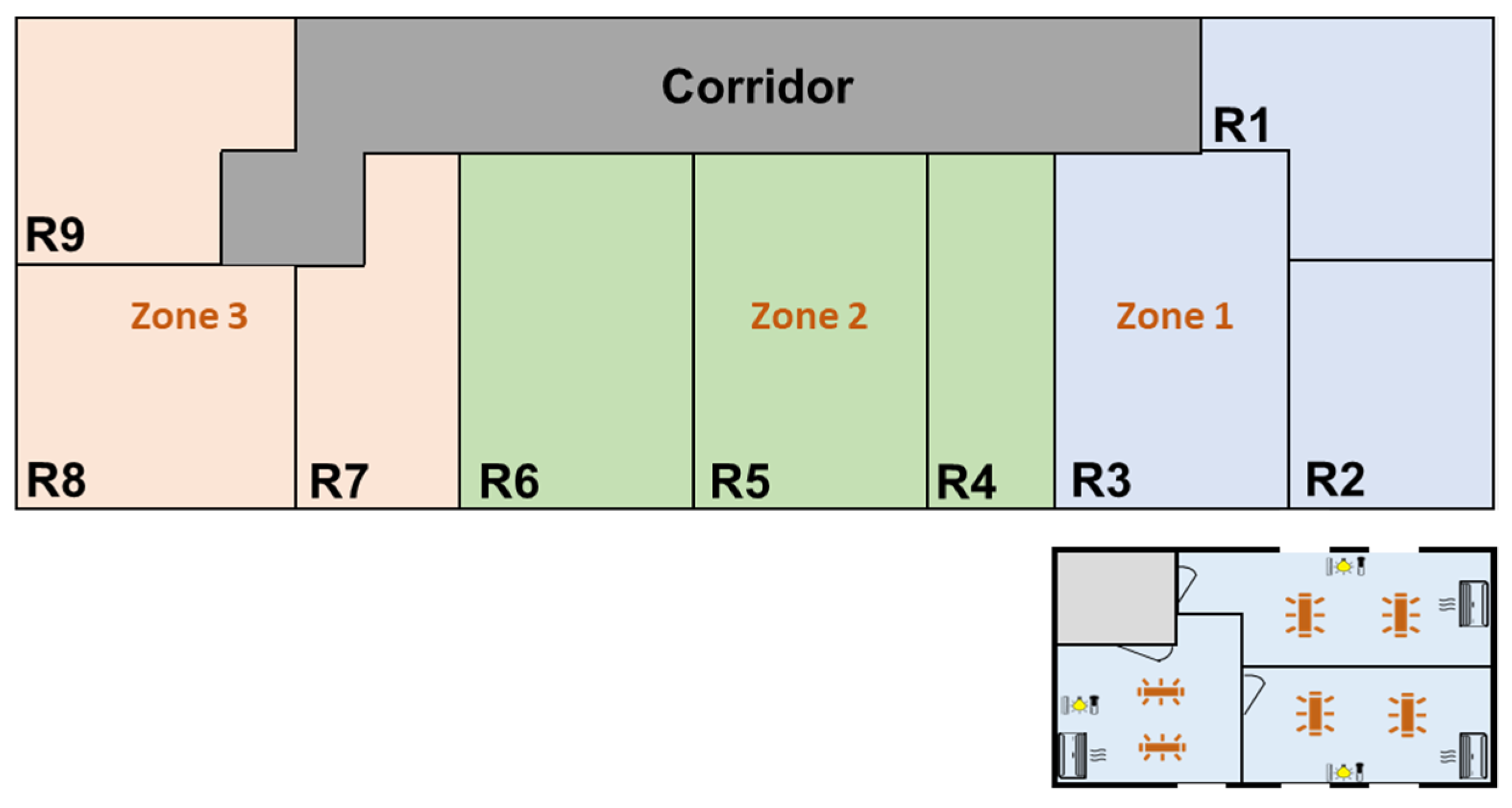
This section presents the case study, including scenarios and the respective results. The building’s historical data have been used as input data, so that the building has been divided into three zones [1]. In Figure 2, the topology of the building can be seen, with the respective three zones and the nine rooms (R1 to R9). In the bottom-right of Figure 2 is shown the detail of Zone 1. The zones of the building have been defined according to the sub-metering installed in the building. It matches the electrical switchboard coverage zones. In this way, the sensors data and consumption data are aggregated according to these zones. For this case study, the historical data of Zone 1 are selected. The selected historical data span the period from 22 May 2017 to 17 November 2019 with 5 min time intervals. It should be noted that the building is equipped with energy meters to record the consumption data and PV generation data as well. Additionally, there are different building sensors such as seven light power indicators, four movement sensors, three door status indicators, one air quality sensor, one temperature sensor, one humidity sensor, and one CO2 sensor.
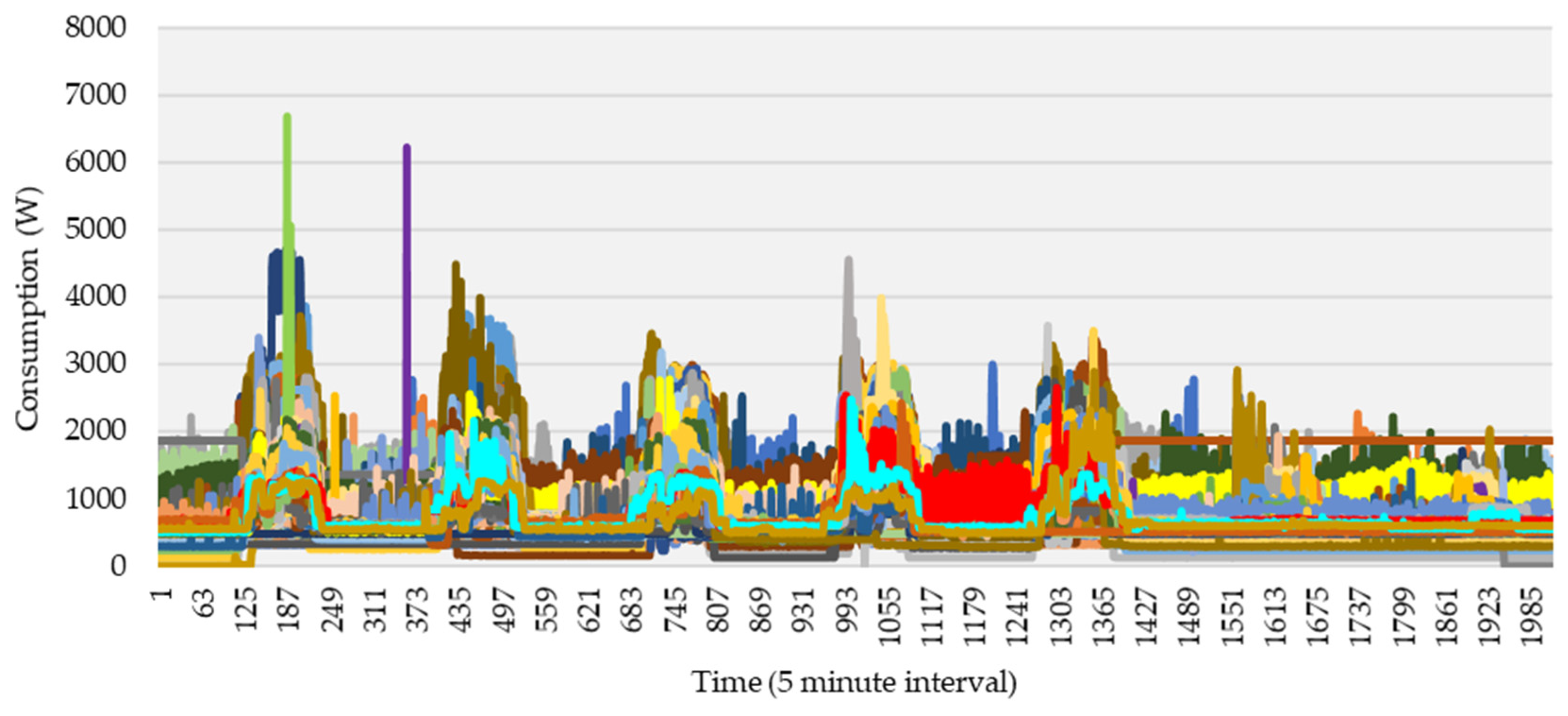
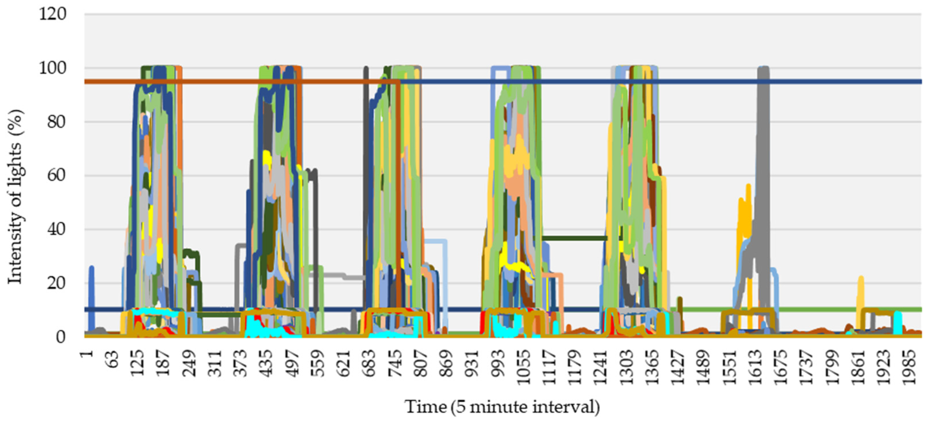
The input data are a matrix structure composed of twelve columns evidencing attributes associated to specific five-minute periods. A total of 262,060 rows evidencing the total number of observations from 22 May 2017 to 17 November 2019 were separated by five-minute intervals. The historic dataset represented by 22 May 2017 to 8 November 2019 contains 260,054 rows while the target week represented by 11 to 17 November contains 2006 rows. The initial ten columns identify consumption values, while the remaining two identify additional values obtained from enhanced sensors data, more specifically CO2 and light intensity. The ten-input consumption featuring five-minute field values that precede the output counterpart corresponds to a period of fifty minutes. The CO2 and light intensity resemble a single value placed in the five minutes preceding the output consumption. This dataset has been categorized based on the weeks, so focused time period includes 130 weeks. Figure 3, Figure 4 and Figure 5 show the building’s present input data in 130 weeks, related to the power consumption, CO2 concentration, and intensity of lights, respectively. It means that each line represents the consumption data of one specific week in 2016 periods (5 min time interval).
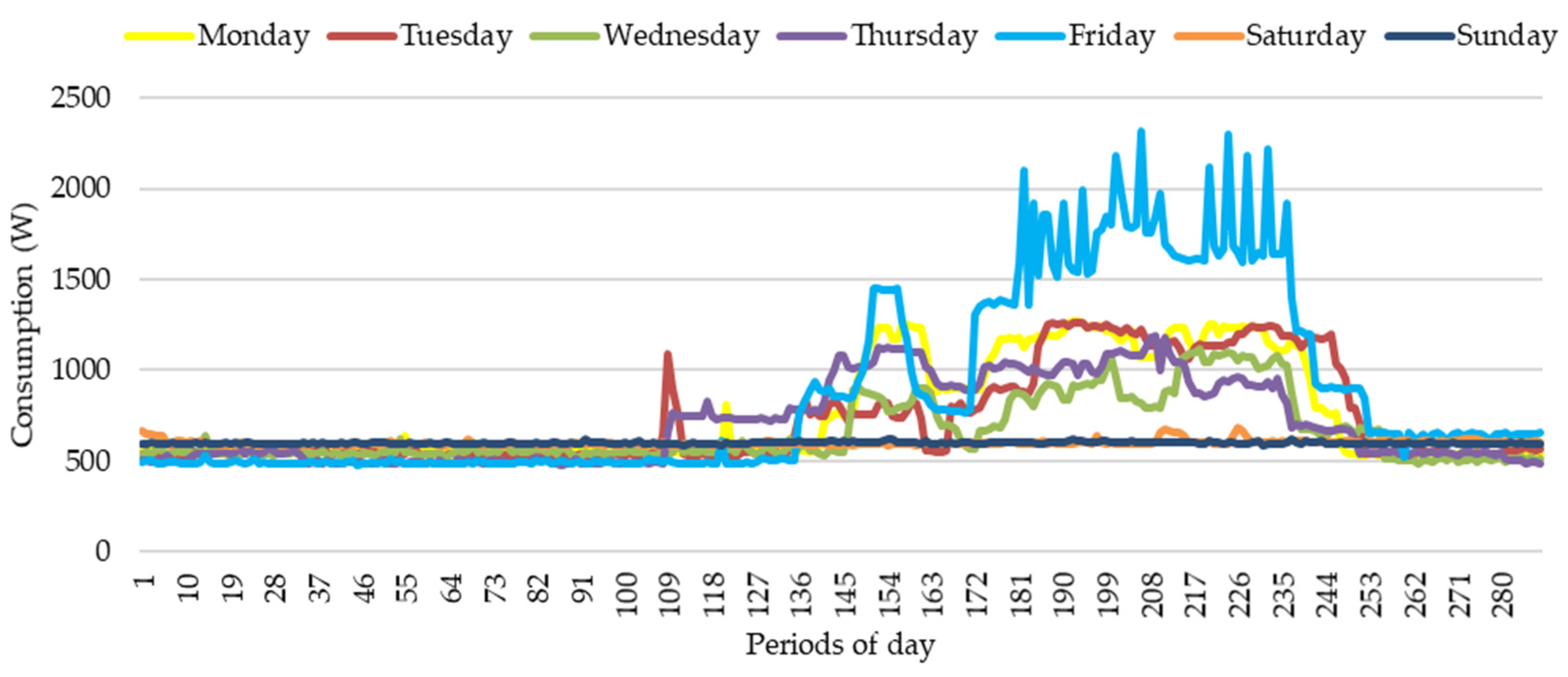
Several other environment data and parameters, such as the weather data, can impact the forecasting model’s accuracy; the authors have discussed this in [1]. It has been concluded that, for the office building under study, as the researchers have a very specific routine, weather data do not contribute to improving the accuracy of the forecasting. This case study’s main purpose is to forecast the consumption of 7 days based on the proposed training dataset. Additionally, 60 scenarios have been tested on different parameters such as number of entries, learning rate, number of neurons, clipping ratio, epochs, early stopping, and validation split on the forecasting results. Figure 6 shows the real consumption of 7 days of the test dataset. It should be noted that each day includes 288 periods (5 min interval), and each color represents one day.
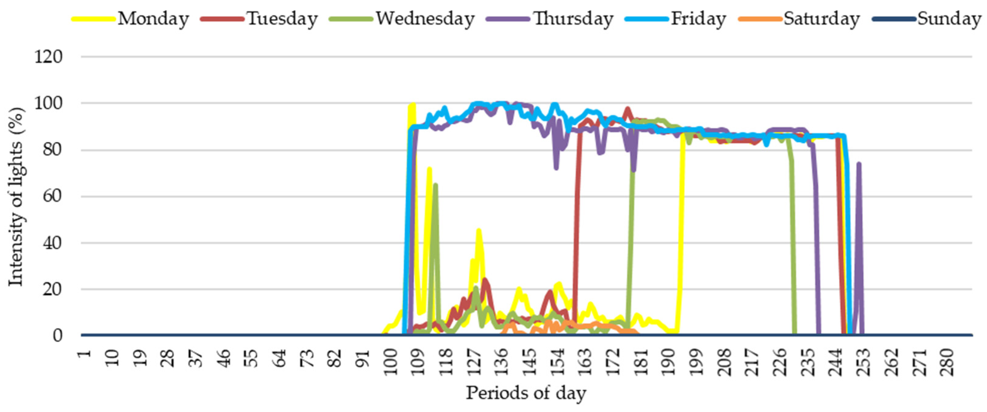
The CO2 concentration and intensity of lights have been presented in Figure 7 and Figure 8, respectively, to propose the real data in the last week.
Table 1 introduces the characteristics of 60 scenarios with different parameters. Additionally, the calculated error of each forecasting can be seen on the right side of the table based on the ANN and KNN approaches. As shown in Table 1, the rank of calculated errors has been presented by dark color to bright color so that dark green cells show the lower error and white cells present the higher errors. To present the details of these error calculations, three scenarios (A, B, and C) have been selected to be illustrated by figures. The characteristics of these three cases can be seen in Table 1. The characteristics of scenarios A and C are equal. However, the applied techniques for the forecast are different.
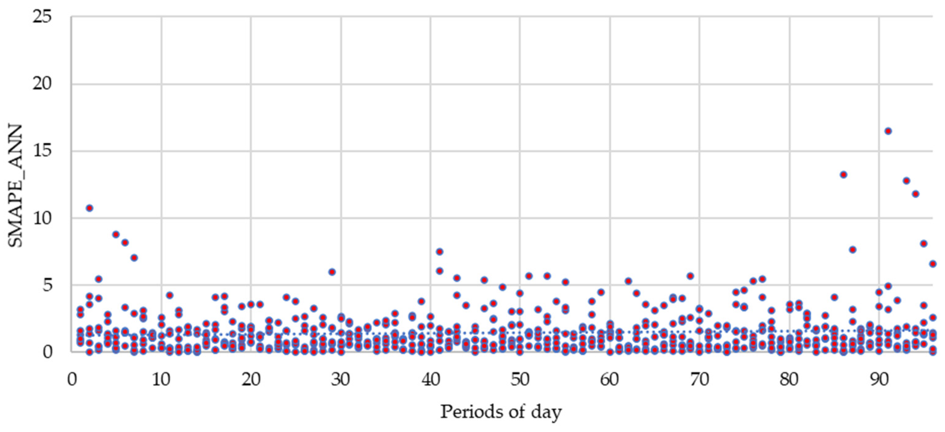
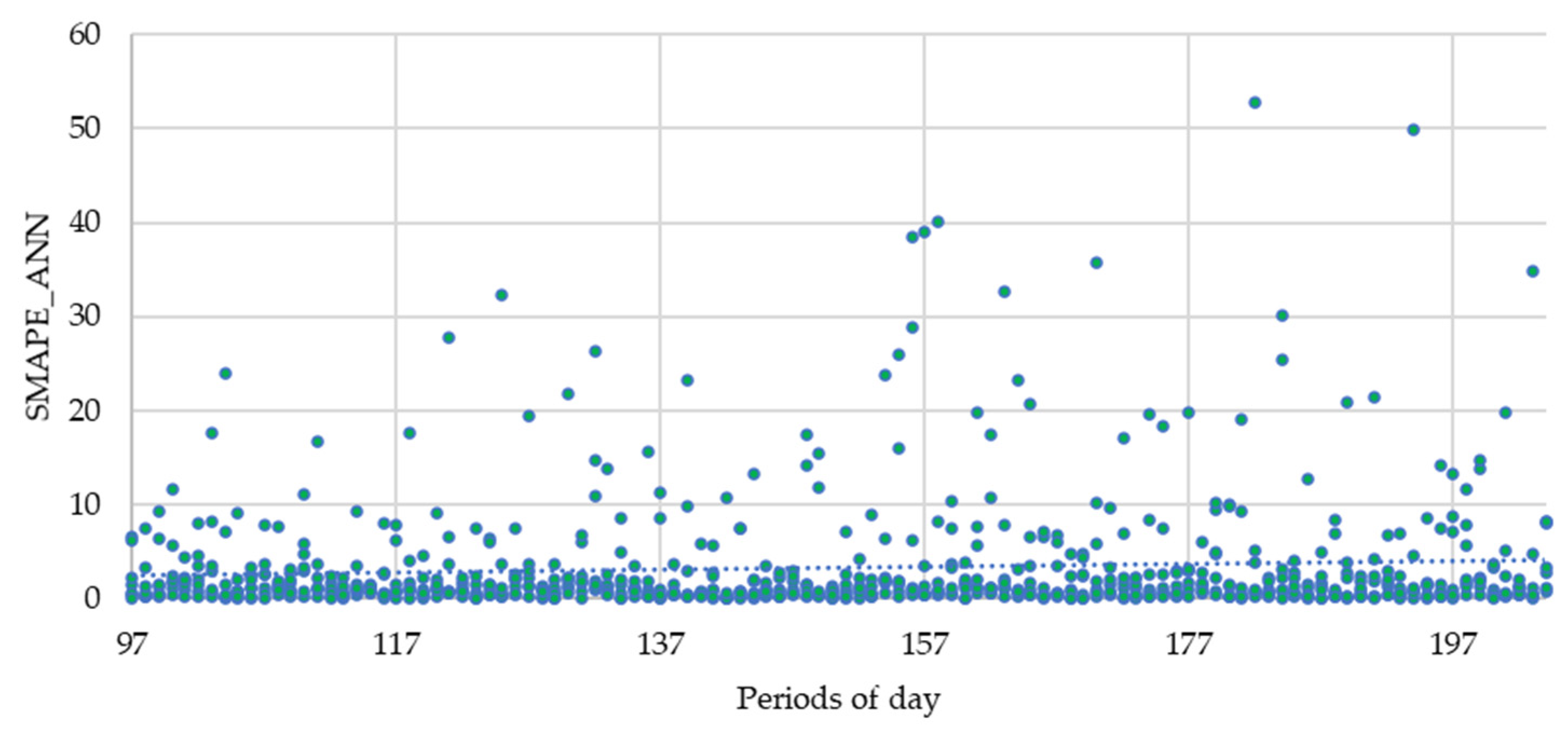
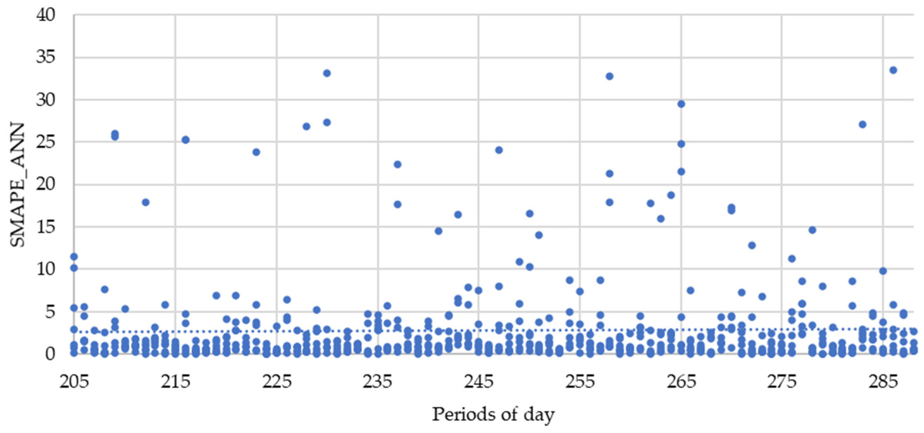
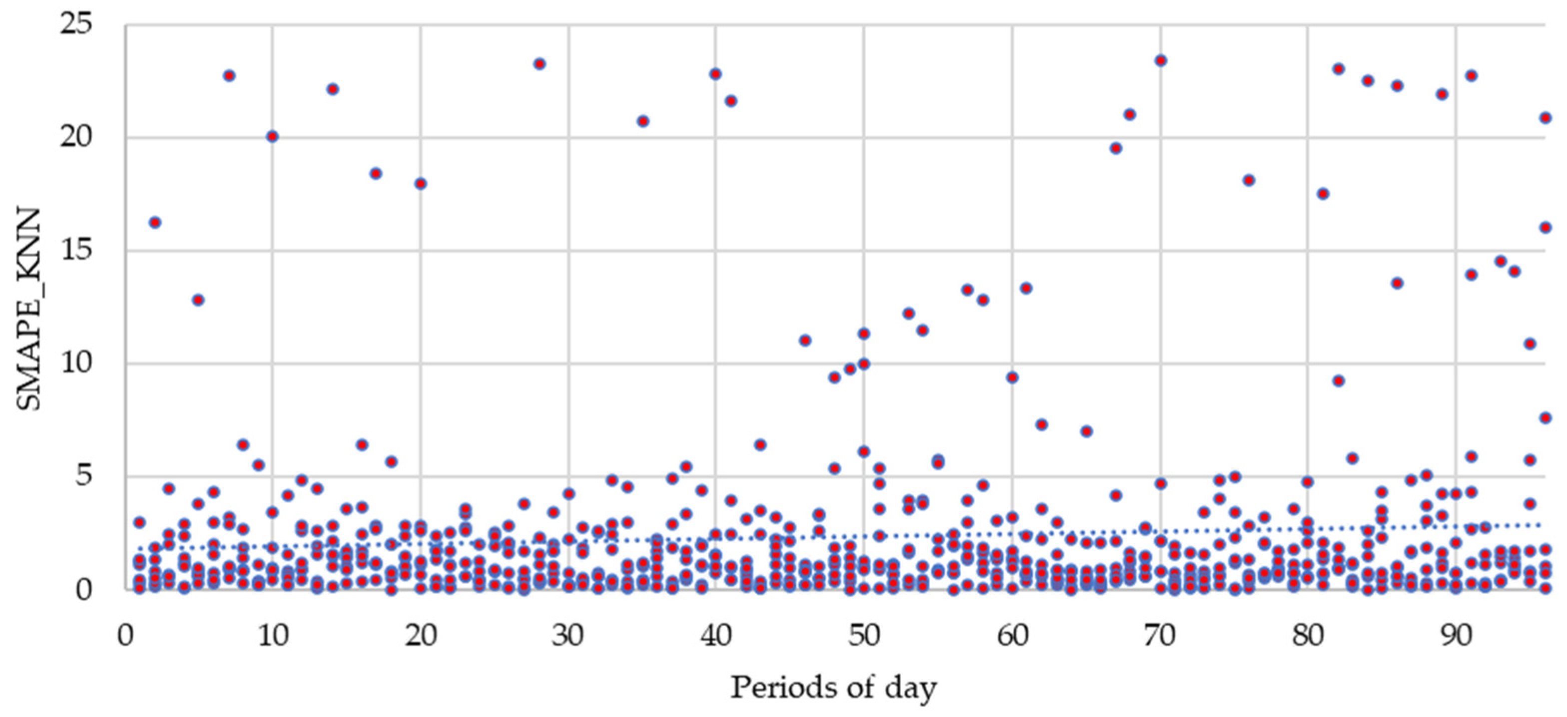
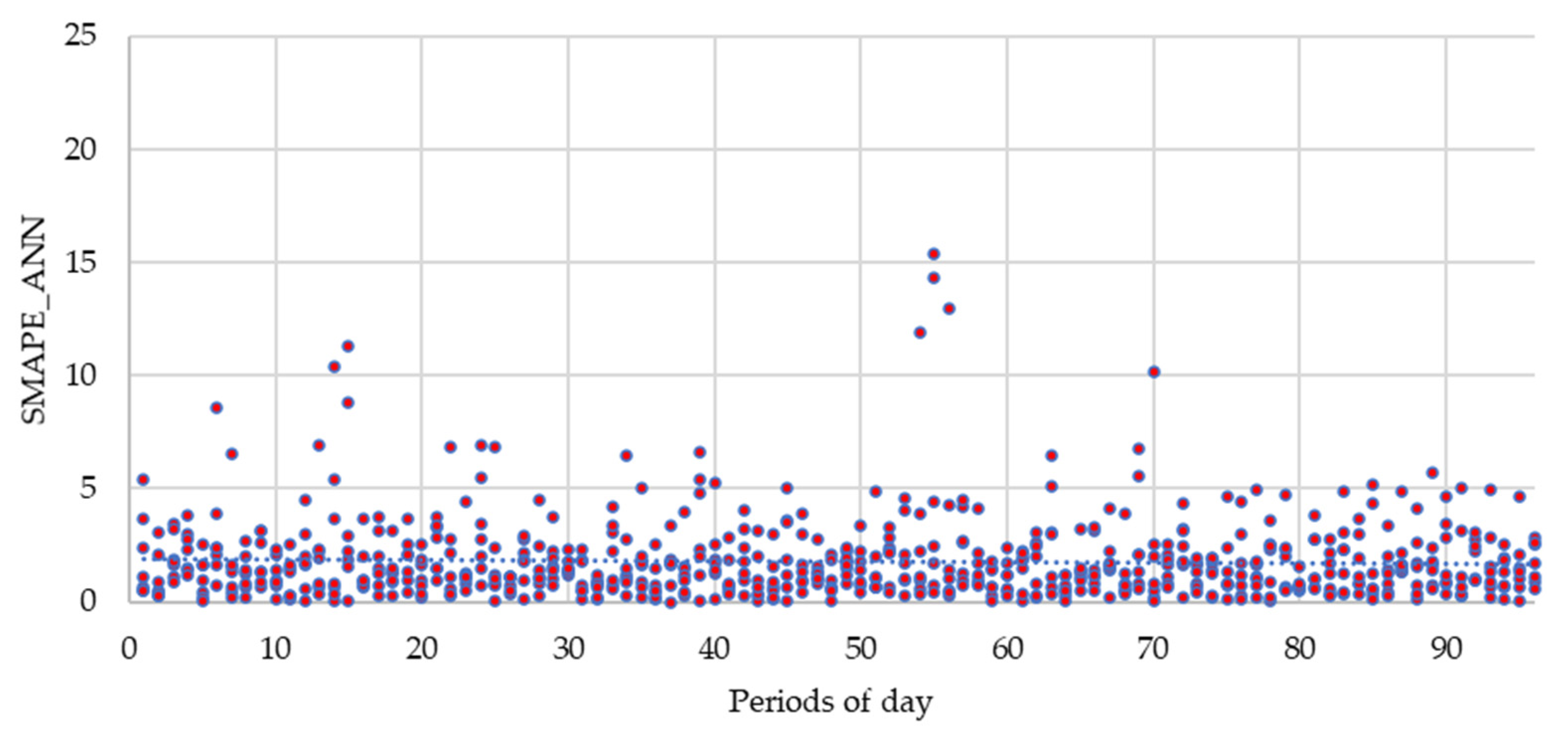
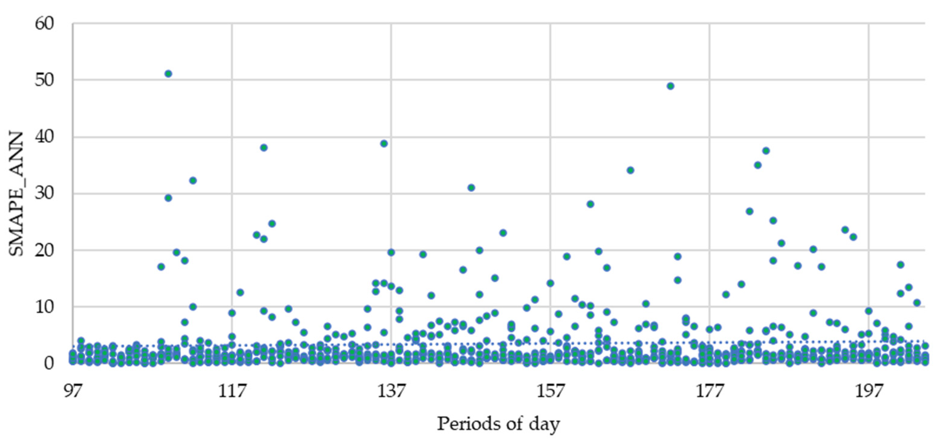
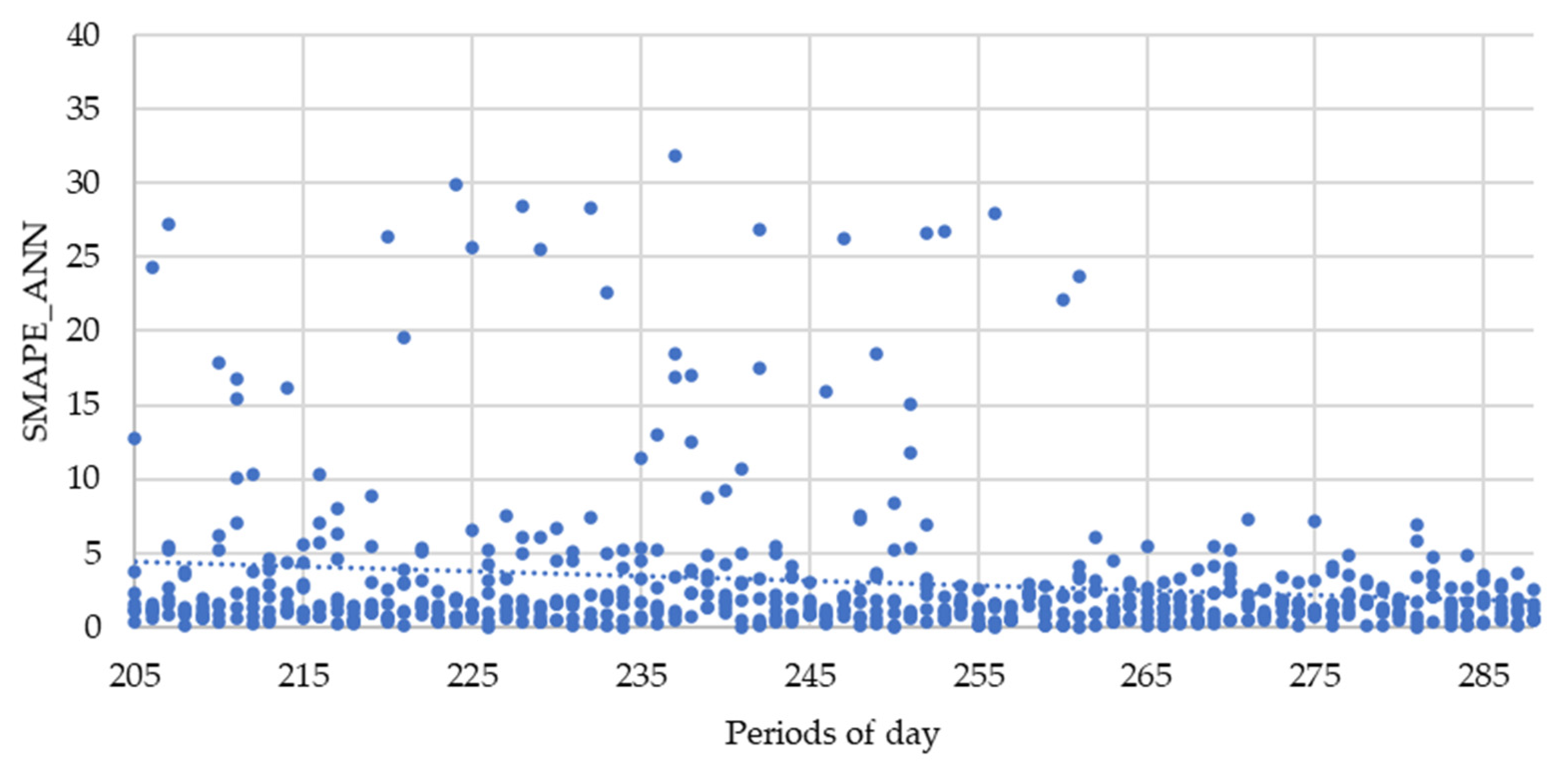
Each scenario focuses on seven days, shown by three figures based on the focused time. Figure 9 indicates 96 periods related to the 00:00 to 08:00 (5 min time interval), Figure 10 focuses on 108 periods from 08:00 to 17:00 (5 min time interval), and Figure 11 is related to the 84 periods from 17:00 to 24:00 (5 min time interval). The three referenced figures are related to scenario A. In Appendix A, the figures are presented related to scenario B (Figure A1, Figure A2 and Figure A3) and the figures related to scenario C (Figure A4, Figure A5 and Figure A6). The values selected for each parameter have been defined by the authors based on the experiments made on the ranges of each parameter that affect the results of forecasting. Additionally, the authors wanted to determine the influence of using the day-of-the-week information as input data to decide if it contributes or not to improving the accuracy.
Figure 9 presents the calculated SMAPE of scenario A in the first part of the day: 96 periods of 5 min are presented, related to the period between 00:00 and 08:00.
Each period of 5 min includes seven points in the graph, corresponding to the consumption for seven days of the week. Figure 10 presents the calculated SMAPE of scenario A in the second part of the day (from 08:00 to 17:00). Figure 11 presents the calculated SMAPE of scenario A in the third part of the day.
The discussion of the results obtained will be presented in Section 4, focusing on the results already presented and Appendix A.
Regarding the error analysis in each day, Table 2 presents the SMAPE errors for each method. The data used in Table 2 relate to ten entries: learning rate (0.005), number of neurons in intermediate layers (64), clipping ratio (5.0), number of epochs (500), early stopping (20), validation split (0.2). The day of the week is not considered.
It can be seen that for every single day, ANN is always providing a more accurate forecast. However, as can be seen in the period-by-period analysis, KNN can have better accuracy in specific periods of the day or week.

4. Discussion

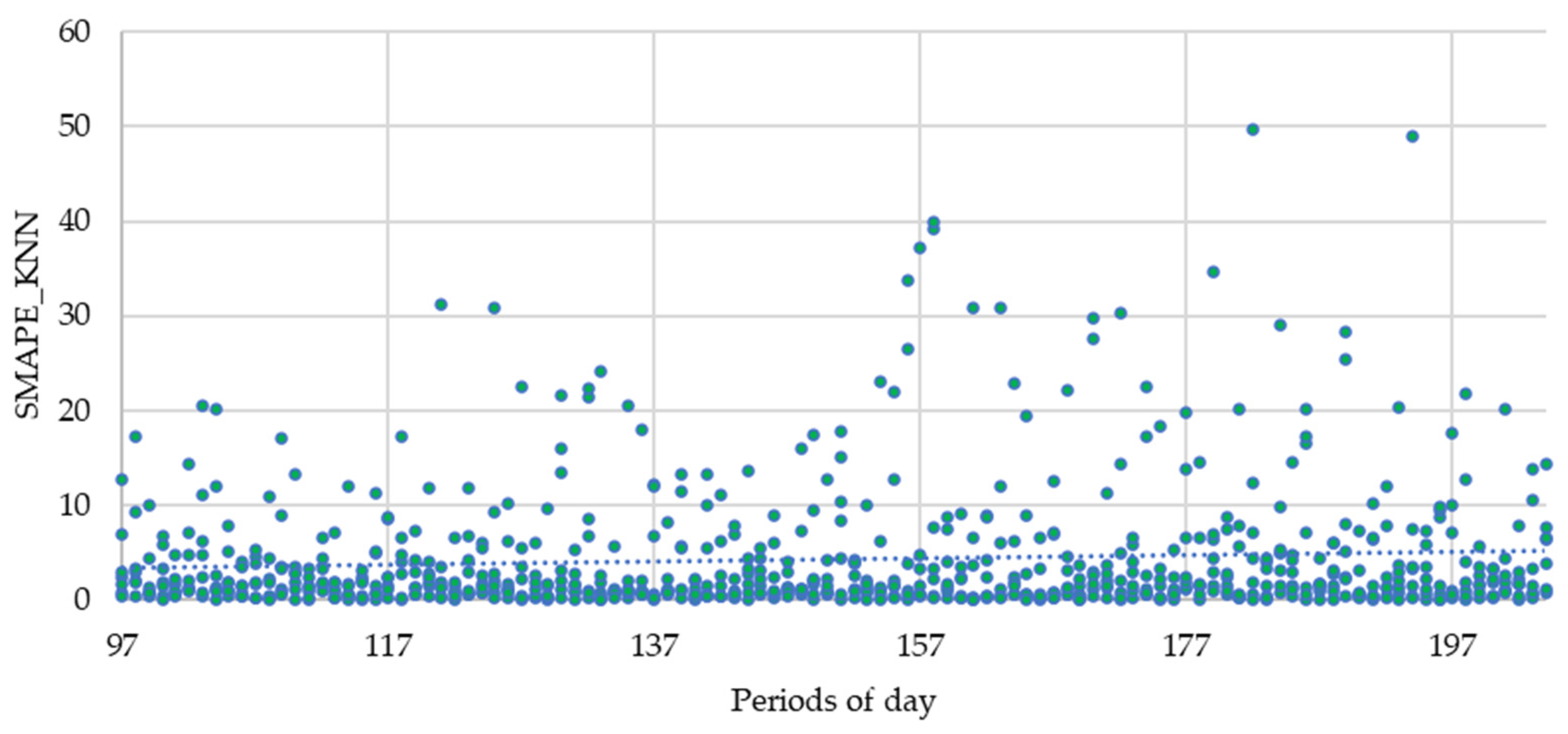
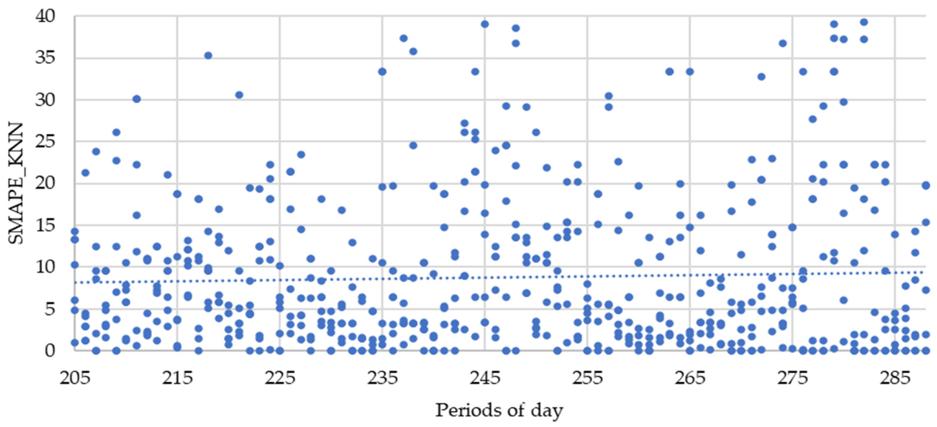
Looking at Figure 9, Figure 10 and Figure 11 and Figure A1, Figure A2, Figure A3, Figure A4, Figure A5 and Figure A6 it is possible to see that the same method with the same parameters is not more accurate for all the periods. Focusing on the first period of the day, from 00:00 to 08:00, it can be seen that scenario C is the one with the highest dispersion of SMAPE for each period. Looking at Table 1, scenario C is the one with higher SMAPE between the three scenarios. However, for the period between 08:00 and 17:00, scenario C’s results are not the worst ones, mainly compared with scenario A (Figure 9 and Figure A2). Finally, regarding the third part of the day, from 17:00 to 24:00, scenario C is the worst one. Scenario B has a regular behavior along this period. However, scenario A is the best one at the end of this period (in the last third of this period). Comparing ANN and KNN, it can be seen that it is impossible to decide on the best one as scenario C is very accurate in a specific period of the day.
It has been found that, generally, the number of entries should be 10, as increasing the number of entries does not provide better results. Regarding the learning rate, it has been found that lower learning rates were more accurate in the results. The same comment applies to the number of neurons. Regarding the clipping ratio and the epochs, the early stopping, the validation split, and the days of the week, it is not possible to make a selection, as both values provide good results in different scenarios.
These results and discussion lead us to conclude that the definition of the ANN and KNN features must be done contextually, as different contexts bring different consumption patterns, and therefore, deserve different configurations in algorithms.

5. Conclusions

This paper has presented a forecasting service used in an office building aiming to support decisions regarding energy management towards efficiency. Two algorithms for forecasting have been used, namely artificial neural network and K-nearest neighbor, testing different algorithms and data features. It has been found that, for different periods of the day, which means different contexts regarding consumption patterns, different algorithm parameters can have higher accuracy levels. This means that it is not possible to say that a single algorithm is more accurate for the office building under study. In other words, one should select KNN for some periods of the day and ANN for other periods of the day, as discussed in Section 4.

Author Contributions

Conceptualization, P.F., and Z.V.; methodology, P.F., Z.V.; software, D.R., M.K.; validation, D.R., P.F., Z.V.; formal analysis, D.R.; investigation, D.R., M.K., P.F., Z.V.; resources, P.F., Z.V.; data curation, D.R., M.K., P.F., Z.V.; writing—original draft preparation, D.R., M.K., P.F., Z.V.; writing—review and editing, D.R., M.K., P.F., Z.V.; visualization, D.R., M.K., P.F.; supervision, P.F., Z.V.; project administration, P.F., Z.V.; funding acquisition, P.F., Z.V. All authors have read and agreed to the published version of the manuscript.

Funding

This work has received funding from FEDER Funds through COMPETE program and from National Funds through (FCT) under the projects UIDB/00760/2020, MAS-Society (PTDC/EEI-EEE/28954/2017) and CEECIND/02887/2017.

Data Availability Statement

The data used in this study are available in [1].

Conflicts of Interest

The authors declare no conflict of interest.

Appendix A

This appendix presents six figures that are added to the results.
Figure A1. Forecast errors based on ANN approach in scenario B from 00:00 to 08:00.
Forecasting 03 00015 g0a1
Figure A2. Forecast errors based on ANN approach in scenario B from 08:00 to 17:00.
Forecasting 03 00015 g0a2
Figure A3. Forecast errors based on ANN approach in scenario B from 17:00 to 24:00.
Forecasting 03 00015 g0a3
Figure A4. Forecast errors based on the KNN approach in scenario C from 00:00 to 08:00.
Forecasting 03 00015 g0a4
Figure A5. Forecast errors based on the KNN approach in scenario C from 08:00 to 17:00.
Forecasting 03 00015 g0a5
Figure A6. Forecast errors based on the KNN approach in scenario C from 17:00 to 24:00.
Forecasting 03 00015 g0a6

References

  1. Ramos, D.; Teixeira, B.; Faria, P.; Gomes, L.; Abrishambaf, O.; Vale, Z. Use of Sensors and Analyzers Data for Load Forecasting: A Two Stage Approach. Sensors 2020, 20, 3524. [Google Scholar] [CrossRef]
  2. Bless, K.; Furong, L. Allocation of Emission Allowances to Effectively Reduce Emissions in Electricity Generation. In Proceedings of the 2009 IEEE Power & Energy Society General Meeting, Calgary, AB, Canada, 26–30 July 2008; pp. 1–8. [Google Scholar] [CrossRef]
  3. Rudnick, H. Environmental impact of power sector deregulation in Chile. In Proceedings of the 2002 IEEE Power Engineering Society Winter Meeting. Conference Proceedings (Cat. No.02CH37309), New York, NY, USA, 27–31 January 2002; Volume 1, p. 392. [Google Scholar] [CrossRef]
  4. Faria, P.; Vale, Z. A Demand Response Approach to Scheduling Constrained Load Shifting. Energies 2019, 12, 1752. [Google Scholar] [CrossRef] [Green Version]
  5. Pop, C.; Cioara, T.; Antal, M.; Anghel, I.; Salomie, I.; Bertoncini, M. Blockchain Based Decentralized Management of Demand Response Programs in Smart Energy Grids. Sensors 2018, 18, 162. [Google Scholar] [CrossRef] [PubMed] [Green Version]
  6. Faria, P.; Vale, Z. Demand response in electrical energy supply: An optimal real time pricing approach. Energy 2011, 36, 5374–5384. [Google Scholar] [CrossRef] [Green Version]
  7. Cao, Y.; Du, J.; Soleymanzadeh, E. Model predictive control of commercial buildings in demand response programs in the presence of thermal storage. J. Clean. Prod. 2019, 218, 315–327. [Google Scholar] [CrossRef]
  8. Law, Y.; Alpcan, T.; Lee, V.; Lo, A. Demand Response Architectures and Load Management Algorithms for Energy-Efficient Power Grids: A Survey. In Proceedings of the 2012 7th International Conference on Knowledge, Information and Creativity Support Systems, KICSS 2012, Melbourne, Australia, 8–10 November 2012; pp. 134–141. [Google Scholar] [CrossRef]
  9. Abrishambaf, O.; Faria, P.; Vale, Z. Application of an optimization-based curtailment service provider in real-time simulation. Energy Inform. 2018, 1, 1–17. [Google Scholar] [CrossRef] [Green Version]
  10. Marzband, M.; Ghazimirsaeid, S.S.; Uppal, H.; Fernando, T. A real-time evaluation of energy management systems for smart hybrid home Microgrids. Electr. Power Syst. Res. 2017, 143, 624–633. [Google Scholar] [CrossRef]
  11. Allen, J.; Snitkin, E.; Nathan, P.; Hauser, A. Forest and Trees: Exploring Bacterial Virulence with Genome-wide Association Studies and Machine Learning. Trends Microbiol. 2021. [Google Scholar] [CrossRef] [PubMed]
  12. Kilincer, I.; Ertam, F.; Sengur, A. Machine Learning Methods for Cyber Security Intrusion Detection: Datasets and Comparative Study. Comput. Netw. 2021, 188, 107840. [Google Scholar] [CrossRef]
  13. Trivedi, S. A study on credit scoring modeling with different feature selection and machine learning approaches. Technol. Soc. 2020, 63, 101413. [Google Scholar] [CrossRef]
  14. Merghadi, A.; Yunus, A.; Dou, J.; Whiteley, J.; ThaiPham, B.; Bui, D.; Avtar, R.; Abderrahmane, B. Machine learning methods for landslide susceptibility studies: A comparative overview of algorithm performance. Earth Sci. Rev. 2020, 207, 103225. [Google Scholar] [CrossRef]
  15. Jozi, A.; Ramos, D.; Gomes, L.; Faria, P.; Pinto, T.; Vale, Z. Demonstration of an Energy Consumption Forecasting System for Energy Management in Buildings. In Progress in Artificial Intelligence, EPIA 2019, Lecture Notes in Computer Science; Springer: Cham, Switzerland, 2019; p. 11804. [Google Scholar]
  16. Chen, G.H.; Shah, D. Explaining the success of nearest neighbor methods in prediction. Found. Trends Mach. Learn. 2018, 10, 337–588. [Google Scholar] [CrossRef]
  17. Matsumoto, T.; Kitamura, S.; Ueki, Y.; Matsui, T. Short-term load forecasting by artificial neural networks using individual and collective data of preceding years. In Proceedings of the Second International Forum on Applications of Neural Networks to Power Systems, Yokohama, Japan, 19–22 April 1993; pp. 245–250. [Google Scholar] [CrossRef]
  18. Barrash, S.; Shen, Y.; Giannakis, G.B. Scalable and Adaptive KNN for Regression Over Graphs. In Proceedings of the 2019 IEEE 8th International Workshop on Computational Advances in Multi-Sensor Adaptive Processing (CAMSAP), Le Gosier, Guadeloupe, 15–18 December 2019; pp. 241–245. [Google Scholar]
  19. Liu, S.; Zhou, F. On stock prediction based on KNN-ANN algorithm. In Proceedings of the 2010 IEEE Fifth International Conference on Bio-Inspired Computing: Theories and Applications (BIC-TA), Changsha, China, 23–26 September 2010; pp. 310–312. [Google Scholar]
  20. Xie, J.; Liu, B.; Lyu, X.; Hong, T.; Basterfield, D. Combining load forecasts from independent experts. In Proceedings of the 2015 North American Power Symposium (NAPS), Charlotte, NC, USA, 4–6 October 2015; pp. 1–5. [Google Scholar]
  21. Imdad, U.; Ahmad, W.; Asif, M.; Ishtiaq, A. Classification of students results using KNN and ANN. In Proceedings of the 2017 13th International Conference on Emerging Technologies (ICET), Islamabad, Pakistan, 27–28 December 2017; pp. 1–6. [Google Scholar]
  22. González-Vidal, A.; Jiménez, F.; Gómez-Skarmeta, A.F. A methodology for energy multivariate time series forecasting in smart buildings based on feature selection. Energy Build 2019, 196, 71–82. [Google Scholar] [CrossRef]
  23. Ahmad, T.; Zhang, H.; Yan, B. A review on renewable energy and electricity requirement forecasting models for smart grid and buildings. Sustain. Cities Soc. 2020, 55, 102052. [Google Scholar] [CrossRef]
  24. Ahmad, T.; Huanxin, C.; Zhang, D.; Zhang, H. Smart energy forecasting strategy with four machine learning models for climate-sensitive and non-climate sensitive conditions. Energy 2020, 198, 117283. [Google Scholar] [CrossRef]
  25. Bourdeau, M.; Zhai, X. qiang, Nefzaoui, E.; Guo, X.; Chatellier, P. Modeling and forecasting building energy consumption: A review of data-driven techniques. Sustain. Cities Soc. 2019, 48, 101533. [Google Scholar] [CrossRef]
  26. Yaïci, W.; Krishnamurthy, K.; Entchev, E.; Longo, M. Internet of Things for Power and Energy Systems Applications in Buildings: An Overview. In Proceedings of the 2020 IEEE International Conference on Environment and Electrical Engineering and 2020 IEEE Industrial and Commercial Power Systems Europe (EEEIC/I&CPS Europe), Madrid, Spain, 9–12 June 2020; pp. 1–6. [Google Scholar] [CrossRef]
  27. Marinakis, V.; Doukas, H. An Advanced IoT-based System for Intelligent Energy Management in Buildings. Sensors 2018, 18, 610. [Google Scholar] [CrossRef] [PubMed] [Green Version]
  28. Jayasuriya, D.; Rankin, M.; Jones, T.; Hoog, J.; Thomas, D.; Mareels, I. Modeling and validation of an unbalanced LV network using Smart Meter and SCADA inputs. In Proceedings of the IEEE 2013 Tencon—Spring, Sydney, NSW, Australia, 17–19 April 2013; pp. 386–390. [Google Scholar] [CrossRef]
  29. Gomes, L.; Sousa, F.; Vale, Z. An Intelligent Smart Plug with Shared Knowledge Capabilities. Sensors 2018, 18, 3961. [Google Scholar] [CrossRef] [PubMed] [Green Version]
  30. Shah, I.; Iftikhar, H.; Ali, S. Modeling and Forecasting Medium-Term Electricity Consumption Using Component Estimation Technique. Forecasting 2020, 2, 163–179. [Google Scholar] [CrossRef]
  31. Nespoli, A.; Ogliari, E.; Pretto, S.; Gavazzeni, M.; Vigani, S.; Paccanelli, F. Electrical Load Forecast by Means of LSTM: The Impact of Data Quality. Forecasting 2021, 3, 91–101. [Google Scholar] [CrossRef]
  32. Keras. Available online: https://www.tensorflow.org/guide/keras (accessed on 4 May 2020).
  33. K-Neighbors. Available online: https://scikit-learn.org/stable/modules/generated/sklearn.neighbors.KNeighborsRegressor.html (accessed on 4 May 2020).
  34. Leva, S. Editorial for Special Issue: “Feature Papers of Forecasting”. Forecasting 2021, 3, 135–137. [Google Scholar] [CrossRef]
  35. Faria, P.; Vale, Z.; Baptista, J. Constrained consumption shifting management in the distributed energy resources scheduling considering demand response. Energy Convers. Manag. 2015, 93, 309–320. [Google Scholar] [CrossRef] [Green Version]
  36. Vale, Z.; Morais, H.; Faria, P.; Ramos, C. Distribution system operation supported by contextual energy resource management based on intelligent SCADA. Renew. Energy 2013, 52, 143–153. [Google Scholar] [CrossRef] [Green Version]
  37. Armstrong, J.S. Long-Range Forecasting from Crystal Ball to Computer; Wiley: Hoboken, NJ, USA, 1985. [Google Scholar]
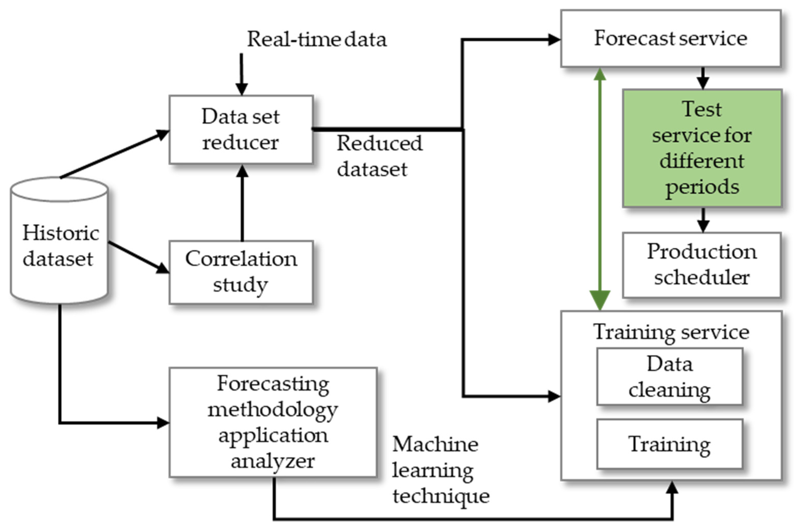
Figure 1. Proposed methodology diagram.
Forecasting 03 00015 g001
Figure 2. Building zones.
Forecasting 03 00015 g002
Figure 3. Power consumption of building from 22 May 2017 to 17 November 2019 is categorized based on the weeks.
Forecasting 03 00015 g003
Figure 4. CO2 concentration data from 22 May 2017 to 17 November 2019 are categorized based on the weeks.
Forecasting 03 00015 g004
Figure 5. Light intensity data from 22 May 2017 to 17 November 2019 are categorized based on the weeks.
Forecasting 03 00015 g005
Figure 6. Actual power consumption of 7 days of the week with 5-minute time intervals.
Forecasting 03 00015 g006
Figure 7. CO2 concentration data of 7 days of the week with 5 min time intervals.
Forecasting 03 00015 g007
Figure 8. Light intensity data of 7 days of the week with 5 min time intervals.
Forecasting 03 00015 g008
Figure 9. Forecast errors based on ANN approach in scenario A from 00:00 to 08:00.
Forecasting 03 00015 g009
Figure 10. Forecast errors based on ANN approach in scenario A from 08:00 to 17:00.
Forecasting 03 00015 g010
Figure 11. Forecast errors based on ANN approach in scenario A from 17:00 to 24:00.
Forecasting 03 00015 g011
Table 1. Error calculation based on artificial neural network (ANN) and K-nearest neighbour (KNN) approaches for 60 different scenarios.
Learn. Rate# NeuronsClipping RatioEpochsEarly StoppingValidation SplitDays of the WeekSMAPE_ANN
(Entries)
SMAPE_KNN
(Entries)
10501001050100
0.001325500200.22.77 *2.754.143.60 ***5.277.57
0.001325500200.2x3.372.735.833.615.277.57
0.001326200100.32.755.753.293.605.277.57
0.001326200100.3x2.53 **3.635.243.615.277.57
0.0011285500200.23.633.525.973.605.277.57
0.0011285500200.2x2.562.723.723.615.277.57
0.0011286200100.34.173.073.983.605.277.57
0.0011286200100.3x3.383.103.443.615.277.57
0.005325500200.26.263.975.413.605.277.57
0.005325500200.2x2.788.645.293.615.277.57
0.005326200100.35.316.427.763.605.277.57
0.005326200100.3x3.662.746.943.615.277.57
0.0051285500200.24.314.663.993.605.277.57
0.0051285500200.2x4.044.216.743.615.277.57
0.0051286200100.34.264.248.113.605.277.57
0.0051286200100.3x6.365.067.913.615.277.57
0.005645500200.25.104.525.643.605.277.57
0.005645500200.2X3.033.445.943.615.277.57
0.005646200100.35.407.006.483.605.277.57
0.005646200100.3x3.494.7911.383.615.277.57
* Scenario A; ** Scenario B; *** Scenario C.
Table 2. SMAPE of ANN and KNN methods for each day.
Method Full PeriodMondayTuesdayWednesdayThursdayFridaySaturdaySunday
ANN2.692.613.043.452.625.161.130.81
KNN3.953.414.944.675.526.851.380.94
Publisher’s Note: MDPI stays neutral with regard to jurisdictional claims in published maps and institutional affiliations.