A Model Predictive Control for the Dynamical Forecast of Operating Reserves in Frequency Regulation Services

Abstract

The intermittent and uncontrollable power output from the ever-increasing renewable energy sources, require large amounts of operating reserves to retain the system frequency within its nominal range. Based on day-ahead load forecasts, many research works have proposed conventional and stochastic approaches to define their optimum margins for reliability enhancement at reasonable production cost. In this work, we aim at delivering real-time load forecasting to lower the operating-reserve requirements based on intra-hour weather update predictors. Based on critical predictors and their historical data, we train an artificial model that is able to forecast the load ahead with great accuracy. This is a feed-forward neural network with two hidden layers, which performs real-time forecasts with the aid of a predictive model control developed to update the recommendations intra-hourly and, assessing their impact and its significance on the output target, it corrects the imposed deviations. Performing daily simulations for an annual time-horizon, we observe that significant improvements exist in terms of decreased operating reserve requirements to regulate the violated frequency. In fact, these improvements can exceed 80% during specific months of winter when compared with robust formulations in isolated power systems.

1. Introduction

The power generation sector has seen rapid growth, mainly due to the increasing industrialization, domestic appliances and transportation demand [1]. The global challenge for modern power systems is to satisfy the growing electricity demand, whilst supplying uninterruptible and high-quality services. For several years now, this requirement has been fulfilled mostly by using fossil fuels because of their concentrated energy, which makes their output dispatchable and easy to adjust according to the load needs [2]. Based on well known load curves, the system operators could appropriately plan-ahead adequate operating reserves to allow for deviation corrections between the expected and actual load demand. However, the continuous burning of fossil-fuels poses a serious threat to the global environment and consequent climate change, calling for emission-free and renewable energy sources in the forthcoming years.

On the other hand, the introduction of renewable power generation produces a number of critical changes on the unit commitment and economic dispatch problem formulation. The intermittent and volatile behavior of renewable resources impose further variations on net demand and thus, the clarity of the operating reserves must be carefully scheduled. In addition, their uncontrollable and unpredictable power output increases the reserve requirements and probable deficits are reflected as frequency deviations between the nominal values. Consequently, the simultaneous increase in electricity demand and reduction in contributions of conventional sources create a lot of power integration and fluctuation issues, which undoubtedly disturb the overall system security, stability and reliability. Since the renewable energy sources do not contribute in flexibility, at a relatively low penetration level, they are commonly treated as negative loads providing comparable fluctuations with the existing net load fluctuations. As their penetration level grows, the conventional generating units occur inadequate for load following [3]. Over the last decade, researchers have extensively applied conventional and stochastic optimization techniques to define the optimal operating reserve margins and enhance the overall system reliability at reasonable costs. Based on predefined load curves, the various approaches broadly used can be divided into robust, deterministic and stochastic. The deterministic formulations recommend constant shares to represent the forecast errors in load demand. Without investigating the comparative performance of different risk considerations, the deterministic approaches rely solely on a set of uncertain parameters, offering poor reliability/cost trade-offs. To strengthen the robustness, a conservative formulation may propose a 5% upward and downward deviation space, while more robust approaches involve up to 10% margins for islanded systems [4]. More recently, a variety of solutions have relied on stochastic mechanisms, distinguishing the formulations into random scenario reduction, distributionally robust and uncertainty-set classifications [5,6]. Aiming at the minimization of the expected cost over a probability distribution that is represented by scenarios, these frameworks are versatile [7,8]. However, they require significant computational efforts and it is difficult to retrieve temporal and spatial correlations within scenario-trees [9].

The vast majority of the literature in relating fields concentrates on household or small area level load forecasting (i.e., distribution transformer) due to the significantly limited availability of regular patterns. In their effort to address the imposed uncertainty, the existing methods can be divided into three main categories. The methods of the first category make use of clustering or classification techniques to correlate similar customers, day types or weather conditions, targeting on the reduction of uncertainty variance [10]. A second category focuses on the elimination of the imposed uncertainties at the meter-level by utilizing aggregated smart-meter data [11], whereas the rest of the methods fall in the last category and refer to uncertainty separation within the regular patterns, relying on spectral analysis such as Fourier transformation, wavelet and empirical mode decomposition [12]. Beyond the aggregated level, load forecasting methods are based on sophisticated mechanisms and machine learning techniques. A tutorial review of probabilistic electric load forecasting is provided in [13]. The authors in [14] presented a comparison between hybrid and artificial intelligence models including support vector machines, expert systems, fuzzy logic, regression trees and artificial neural networks, while the notable time series models of long short-term memory (LSTM) systems, recurrent (RNN) and convolutional (CNN) neural networks combined with different regression techniques are discussed in [15]. Although highly flexible and effective, RNN-based approaches outperform traditional forecasting models in terms of root mean square error (RMSE) and mean absolute percentage error (MAPE) [16,17].

The existing methods aim at day-ahead forecasts or make use of RNN systems to only minimize the forecast error against the actual load. To the best of our knowledge, there has not yet been a comprehensive solution that targets real-time forecasts to improve the performance using updated input values. Most approaches utilize temperature as the only weather-dependent variable and no research work is targeted on the real-time estimation of reserve margins. In this work, we propose a radically different framework to determine the operating reserves based on a real-time load forecast. Identifying their vital role in day-ahead power optimization tasks, we aim at the dynamical update of the predefined daily demand based on a model predictive control. Specifically, we make use of independent input predictors to achieve the dependent target, namely the daily load. Based on annual data with respect to some selected predictors, we train a neural network via non-linear regression. During the particular day, the updated values of the predictors are assigned to the model, which assesses their impact and its significance on the output target and re-use them to estimate the new demand ahead. Together with the power balance, they constitute a system-wide constraint that affects the overall system security and total achieved production cost. The obtained results show that significant improvements exist in terms of decreased operating reserve requirements. Considering the performance of the trained neural network, the determined operating reserves account for the mean squared error (MSE) and the actual deviation of the selected predictors. Based on real-time updates, the load forecasting can achieve lower costs, while the system security is preserved.

The rest of the paper is organized as follows. The following section includes the problem formulation and the importance of accurate reserve definition. Section 3 deals with the methodology followed to develop the proposed, real-time load forecast model. All precise descriptions in relation with the different models used are included. In addition, the considered test system is presented along with the main parameters used for predictions. In Section 4, the realizations of our solution are presented and their findings are discussed in detail, while the obtained improvements are listed by their relevance. Finally, the conclusions are drawn in Section 5.

2. Problem Formulation

In order to achieve a comprehensive view regarding the impact of operating reserves on total generation cost, we first define the generic objective function of unit commitment task with the aid of Equation (1).

$$f=min\sum _{t=1}^T\sum _{i=1}^N\left[F\left(P_i^t\right)+\left(1-U_i^{t-1}\right){SU}_i\right]U_i^t$$

(1)

Denoting the total time intervals with T and the total number of available generating units with N, the power contribution of a generator i during the time slot t is expressed via $P_i^t$·$U_i^t$ defines whether a generator is “on” or “off” during that interval, whereas the cost to start-up is represented by $S{U}_i$. The power balance constraint is provided in Equation (2). In general, the summed power of the committed units must satisfy the load demand $P_d$ [18]. Each deviation from the absolute power balance (zero equivalent) violates the nominal frequency (50 or 60 Hz) of the system according to Newton’s Second Law of Equation (3).

$$\sum _{i=1}^N{U_i^t·P}_i^t=P_d^t$$

(2)

$$T_m-T_e=J\frac{d\omega }{dt}$$

(3)

In case of an imbalance between the mechanical torque $T_m$ and electrical torque $T_e$, the rotating mass will experience an angular acceleration or deceleration $d\omega /dt$, which is reflected as a change in frequency. It is noted that the frequency change is smaller for a system with high inertia (J) compared to a system with low inertia [19]. To guarantee the system stability, different reserve types are needed according to their time of response. For clarification purposes, we express the equation of motion (4) in power terms so that $P=T·\omega$ is preserved.

$$P_m-P_e=M\frac{d\omega }{dt}$$

(4)

where $M=J·\omega$ is the angular momentum of the rotating system. Turning to the specification of the minimum technical and operational characteristics that each user connected to the Transmission System must comply, the frequency range during normal conditions is stated between 49.8 and 50.2 Hz and it can be extended to 47–52 Hz during disturbances. A disturbance event is defined as an incident that causes deviations equal or greater than 0.5 Hz from the nominal $f_o$. The operating reserves are separated into spinning and non-spinning. Spinning reserves are the first acting and derived from the synchronized units to the system [20]. They include the restraint and recovery reserves, which are available within 3 and 20 s and operable for 20 s and 20 min, respectively. Following are the supplemental and replacement reserves which need to be available for 6 h. A last category involves the contingency reserves that are operable within 6–24 h. These categories fall in the non-spinning reserve classification. Day-ahead schedules must satisfy a further system-wide, coupling constraint, namely the spinning reserve margins $S{R}^t$. The formulation of such inequality constraints (both upward $S{R}_{u}p$ and downward $S{R}_{down}$) is expressed via the following respective equations:

$$\sum _{i=1}^N{U_i^t·P}_{i,max}^t\ge P_d^t+{SR}_{up}^t$$

(5)

$$\sum _{i=1}^N{U_i^t·P}_{i,min}^t\le P_d^t-{SR}_{down}^t$$

(6)

where $P_{i,min}$ and $P_{i,max}$ denote the minimum and maximum capacity limits of each generator i. Assuming a robust formulation with SR margins in the order of 10% of the instant load, it is worth noting that this expensive requirement forces more generators to start-up, leading to sub-optimal unit commitment schedules and uneconomic power dispatch.

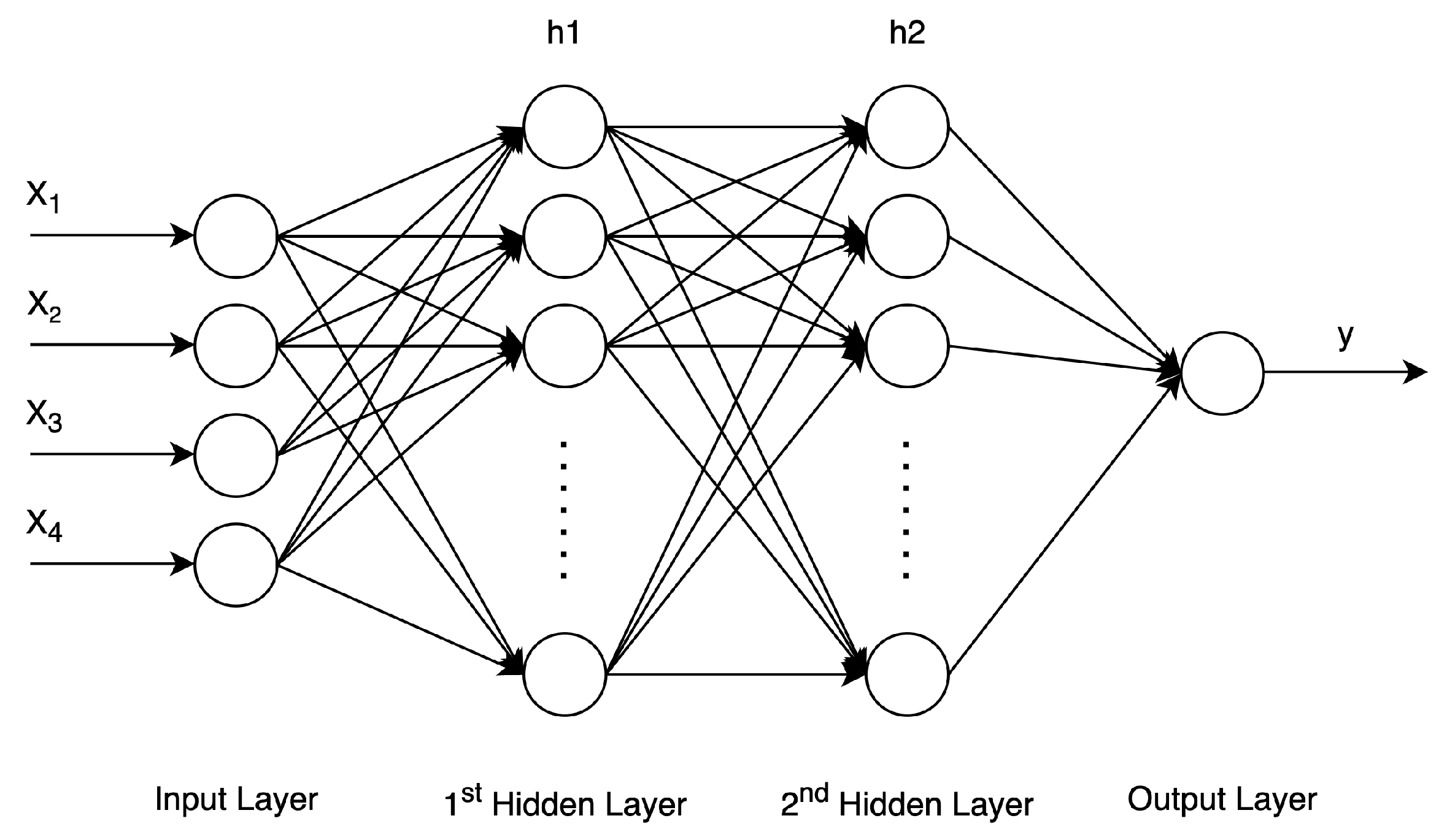
To lower the expensive spinning-reserve requirements, we propose the intra-daily forecast of load demand. In contrast to day-ahead estimations, which may deviate from real-time values, intra-daily forecast with 15 min updates of selected predictors may improve the accuracy and consequent required reserves. Electricity load follows daily patterns, which are repeated according to the human activity and weather conditions. In this regard, we exploit an accurate hours-ahead system for load forecast using neural networks. Our purpose is to enhance the system security and reliability, whilst minimizing the SR requirements by making use of a model predictive control, which performs updates every 15 min to supply the neural networkIn more detail, a number of predictors x are imported in the feed-forward network along with the target y to form our data set $x_i,y_i|i=1,\dots ,n$. The model is trained using the largest share of the historical data for training, while the rest is equally distributed for validation and testing. The developed model exploits a two-hidden-layer neural network employed as follows:

$$h_1=\sigma (\sum _{k=1}^K{w}_k{x}_k+{\beta }_1)$$

(7)

$$h_2=\sigma (\sum _{l=1}^L{w}_l{h}_{1_l}+{\beta }_2)$$

(8)

$$y=\sum _{m=1}^M{w}_m{h}_{2_m}+{\beta }_y$$

(9)

where $\sigma (·)$ is the sigmoid activation function and h the output of the hidden layers. K, L, M are the number of predictors, neurons at the first and second hidden layer, respectively [21]. Figure 1 depicts a graphical representation of the proposed network.

During the realization of power dispatch, the selected predictors $\dot{x}(t)$ re-enter the forecast model at t and the remaining $T-t$ sequence is updated based on the model predictive control explained as follows:

$$I=\sum _{j=t}^T{w}_{x_P}{[r_p(j)-x_p(j)]}^2+\sum _{j=t}^T{w}_y{[\Delta y(j)]}^2$$

(10)

The predicted parameters $r_j$ constitute the reference of the model and each deviation from the actual values is recursively corrected to minimize I·$\Delta y$ indicates the impact of the actual deviation on the new, forecasted values when $x_j$ are reused for load forecast. The significance of $\Delta y$ is regulated by penalizing with $w_y$, while $w_x$ reflects the importance of each selected predictor p. Finally, the equality constraint of $\Sigma w=1$ must be preserved [22,23].

3. Test System and Methodology

The considered system concerns the isolated power community of the island of Cyprus. This is a representative, small-to-medium scale network consisting of 20 generators to supply a 1100 MW peak demand (usually occurred in July) with an annual load factor of 56% [24]. Due to its isolation, small area and remoteness, electricity supply for more than 875 thousand people inhabited in the island, mainly relies on imported fossil fuels, the price of which is 3–4 times higher than that in the mainland [4]. As a result, the extremely high SR requirements of up to 10% of the hourly load pose a critical increase on total production cost. To decide which predictors to include in our forecaster, we first tried to extract a physical relationship between them and our target, namely the load demand. Based on actual data obtained from the Cyprus Energy Regulatory Authority (CERA), we demonstrate the hourly load for a representative week for each season in Figure 2.

Apart from the seasonality and human activity, similar patterns have been observed within the same periods of different years. This way, we choose to express the seasonality by the hour and date, whereas the human activity is represented through the day-type. The repetition of this activity is shown with the aid of three further predictors, such as the daily load of the previous day, week and year. These six predictors form our constant parameters. 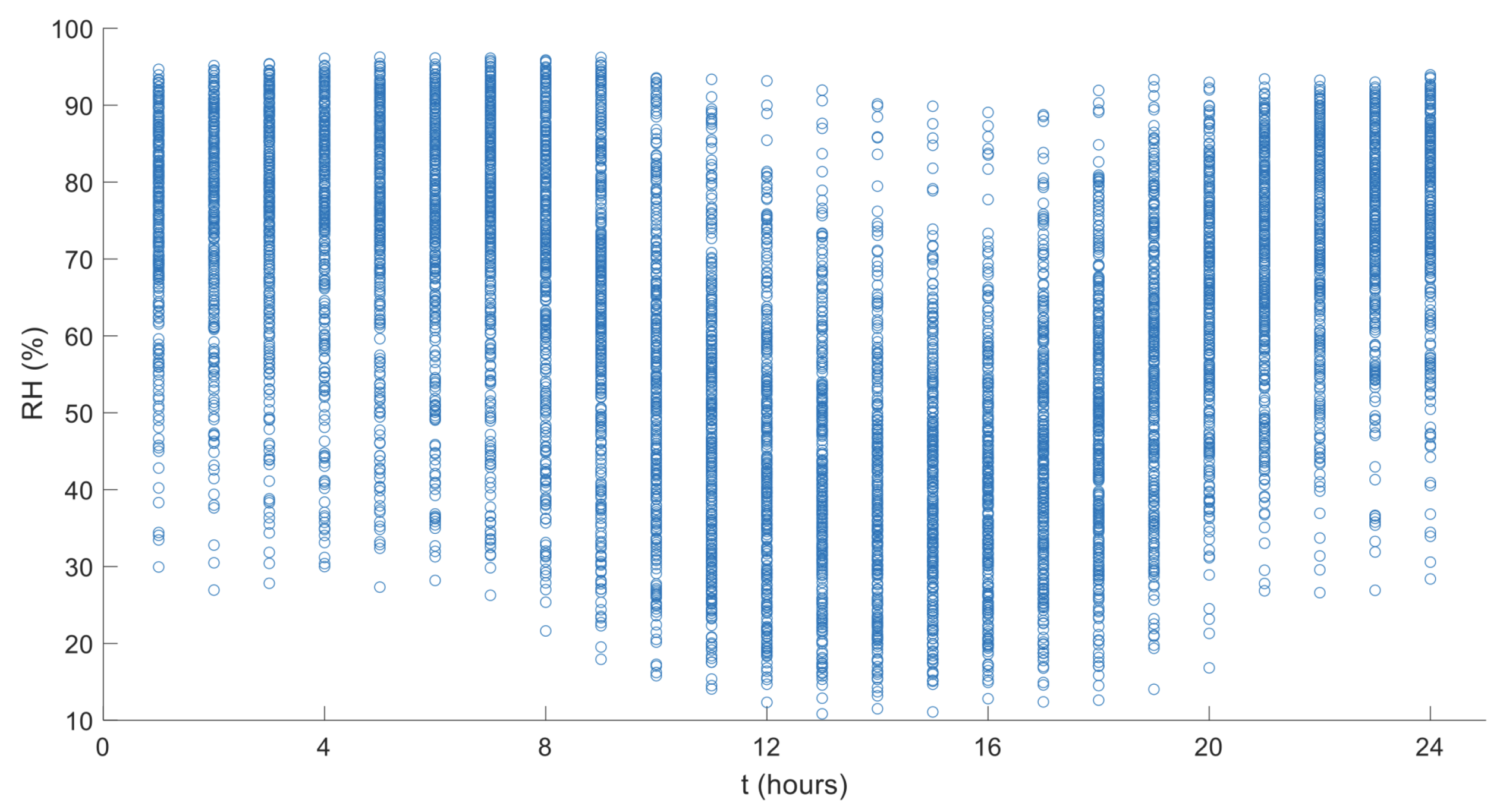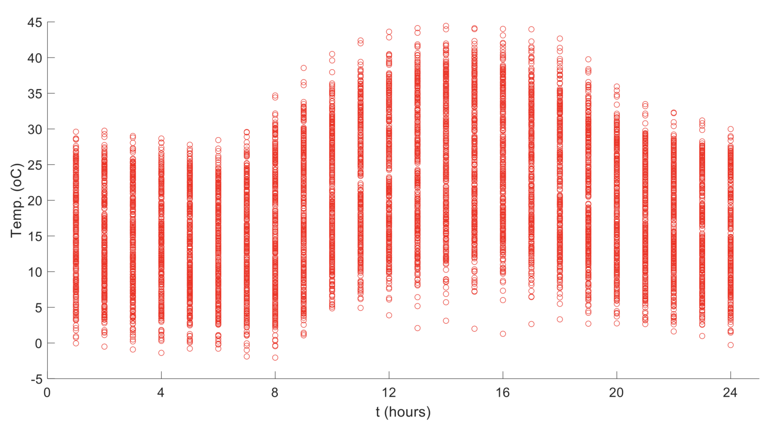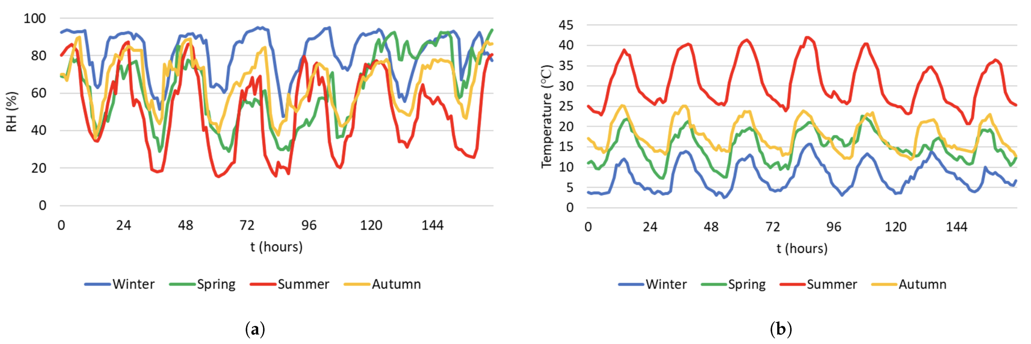In Figure 3, Figure 4 and Figure 5, we provide the fluctuation of temperature and relative humidity which are our further two, variable predictors. Figure 3 and Figure 4 show an hourly histogram relating to the year 2019, while their seasonal values are offered in Figure 5. As can be seen, they both present non-linear relations with time and in order to make easy and accurate predictions, a better resolution is needed. This can be achieved by performing week-to-week comparisons of their hourly variation during different seasons.

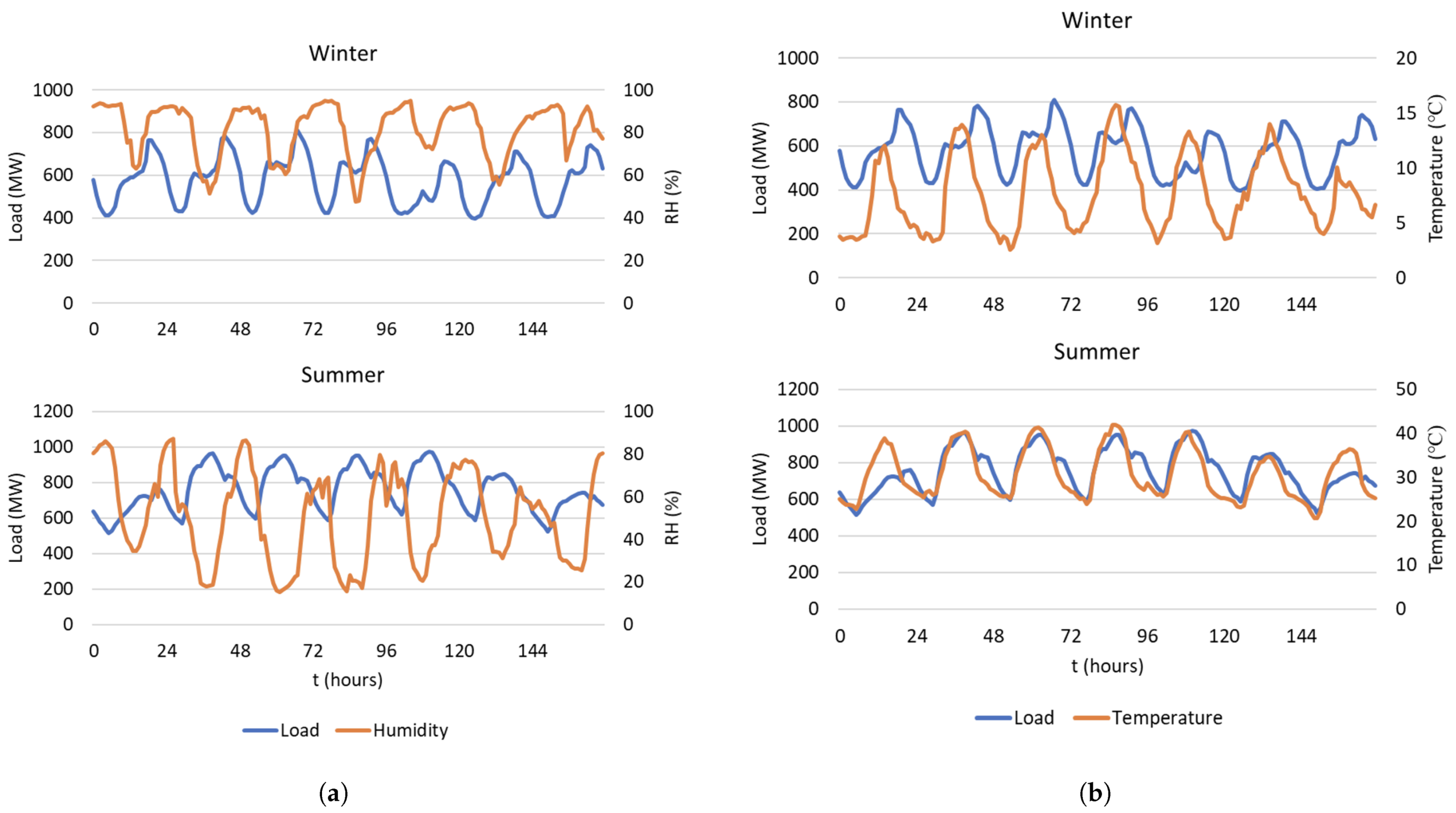
Undoubtedly, ambient temperature affects the human comfort and their overall activity. However, relative humidity is the parameter that ultimately determines the rate with which heat is drawn away from the body and thus how does the absolute temperature “feels like” by humans [25,26]. Figure 6 offers the most important values of temperature and relative humidity for the most energy-intensive weeks in 2019’s winter and summer.

The relative humidity possesses higher values, which tend to decrease during the daylight. On the other hand, the temperature shows an adverse trend, which during the summer shows a linear relationship with load but during winter, it is inversely proportional to the load demand. Therefore, it is obvious that both variables project a fluctuation to load forecast and consequently, they must be updated during the realization of power dispatch. Utilizing actual data from 2010–2019, we train a neural network based on non-linear regression between the following predictors: (1) day (or date), (2) hour, (3) day-type (weekday = 0, weekend = 1, holiday = 2), (4) previous day load, (5) previous week 24h-load, (6) previous year 24h-load, (7) relative humidity and (8) temperature, and the target of actual load demand. The respective settings of our network include 20 neurons per hidden layer. The forecasting model exploits 70% of the historical data for training, 15% for validation and 15% for testing.

Regarding the model used for predictive control, the selected predictors refer to the updated temperature and relative humidity forecasts for the intra-hour periods of 15-minutes, equally weighted by 25%. The remaining 50% is given to the change in the manipulated, depended variable $\Delta y$. In contrast to traditional models that regulate their inputs to approximate the referenced values and minimize their impact, in our realization, we set the updated values as the predicted (reference) and we regulate the controlled temperature and humidity to estimate their impact through the forecaster. Then, the model is updated with the new values and dynamically accepts the updates to perform the next cycle until the end of the assessed day. We illustrate our proposed configuration in Figure 7.

4. Results and Discussion

Aiming at the minimization of expensive SR margins for frequency regulation, we apply our proposed solution introducing the actual data obtained from CERA. We make use of a feed-forward neural network with two hidden layers of 20 neurons and a Levenberg–Marquardt algorithm for the curve fitting. This algorithm relies on the minimization of the squared sum of some imposed parameters $\beta$ [27]. For a given set of n empirical pairs $(x_i,y_i)$, this problem can be formulated as follows:

$$\widehat{\beta }=\underset{\beta }{\mathrm{argmin}}\sum _{i=1}^n{[y_i-f(x_i,\beta )]}^2$$

(11)

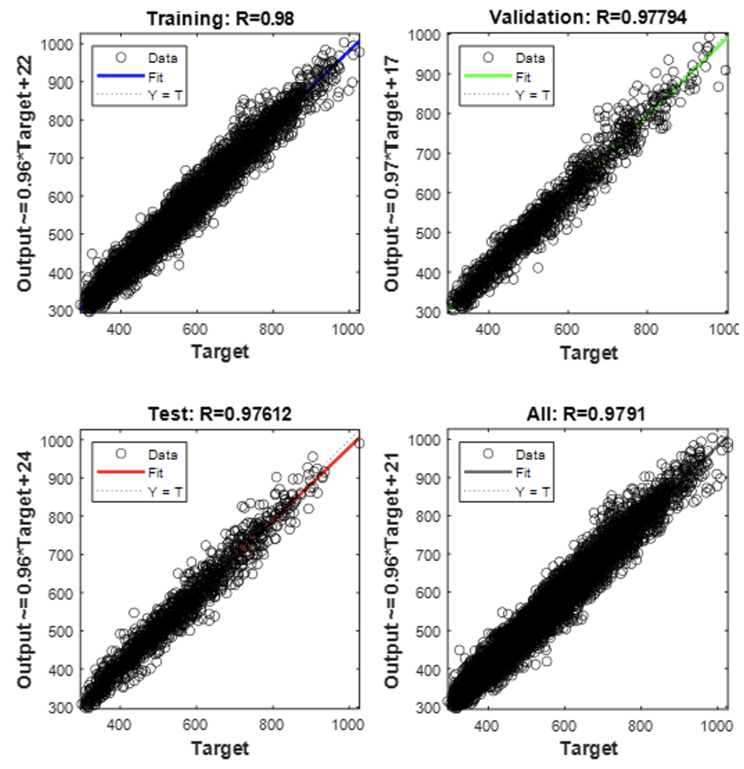
After the introduction of the predictor matrix x (of $nxp$ dimensions) and the dependent target y into the model, the achieved performance of the forecaster is calculated in terms of MSE and presented in Figure 8.

$$MSE=\frac{1}{T}\sum _{t=1}^T{(y_t-{\widehat{y}}_t)}^2$$

(12)

As can be observed, the forecasting model shows high performance with R-values above 97.5% in each case and estimated MSE in the order of 2.388%. The regression plots displayed, show that the network outputs with respect to targets for training, validation, and test sets, fall along the 45-degree line, where the network outputs are equal to the targets. This verifies our views on the existence of lower SR requirements. For further verification of the network performance, we illustrate the error histogram in Figure 9.

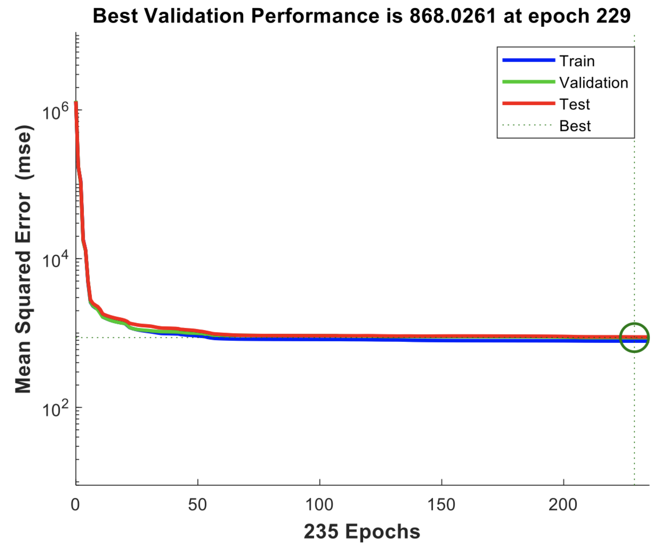
The outliers’ indication shows that most errors fall between −75 and +75. The respective training, validation and test error appear in Figure 10. Since the test set error presents similar characteristics with the validation set error, as well as the final mean squared error being small, the obtained result is quite reasonable.

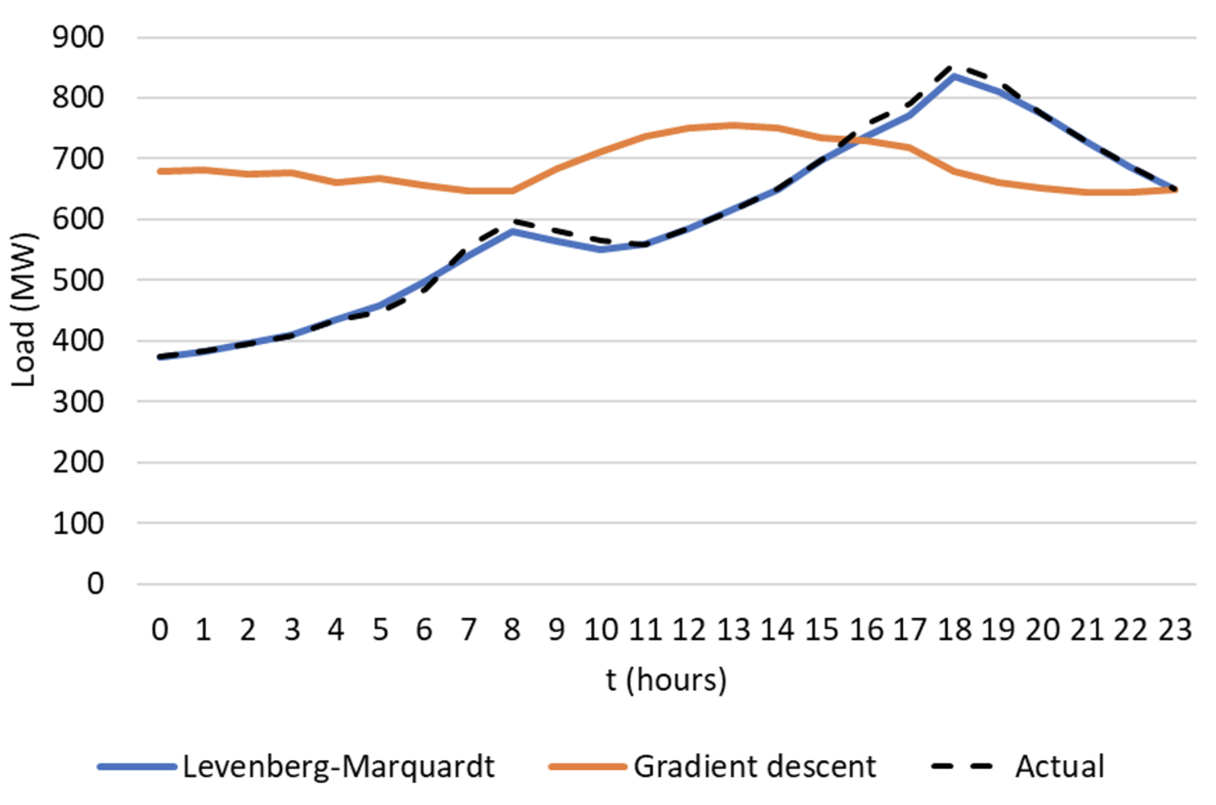
To gain a broader overview of the efficacy of our approach, we compare our proposed solution with a benchmark optimizer, namely Gradient Descent. Based on Equations (13) and (14), the achieved RMSE and MAPE are 10.6227 and 0.0105, respectively, when Levenberg–Marquardt is used, against Gradient Descent, which accounts for 168.4502 RMSE and 0.2875 MAPE. Figure 11 demonstrates the load forecast recommendation for the considered optimizers. Selecting Levenberg–Marquardt as the optimizer for curve fitting, we illustrate the performance of the proposed neural network over the alternative regression trees in Figure 12. Although the proposed solution almost perfectly fits the actual load demand, the alternative regression tree-based approach deviates considerably, providing the respective 68.8261 and 0.0907 RMSE and MAPE.

$$\mathrm{RMSE}=\sqrt{\frac{1}{T}\sum _{t=1}^T{(y_t-{\widehat{y}}_t)}^2}$$

(13)

$$\mathrm{MAPE}=\frac{1}{T}\sum _{t=1}^T\mid \frac{y_t-{\widehat{y}}_t}{y_t}\mid$$

(14)

Applying daily simulations for the entire year of 2020, we estimate the deviation errors between the day-ahead, forecasted load and actual, real-time values during the assessed dates. The input of the model predictive control is updated using intra-hour (15-minutes sampling rates) data regarding the forecasted ambient temperature and relative humidity. The worst deviations are found to be during summer and their actual representation is shown in Figure 13. It is noted that there imposed 24 updates which represent the most prevalent of the 4 intra-hour ones. We depict the most relevant deviations which accounts for over 2% error.

These deviations have a daily impact on the forecasted load, which is reflected as frequency violations. To correct the deviations, more generators are required to serve the varying demand or spinning reserves are called upon. Any generation deficits may lead into load interruptions, while excess generation can cause active power curtailment. In any case, the unexpected deviations increase the total production cost and force the system operators to plan-ahead bulk operating reserves to appropriately regulate the system frequency. In our paradigm, the SR minimization relies on the high-performance neural network and the real-time corrections based on the updated forecasts of temperature and humidity. In contrast to traditional alternatives, which associate the SR requirements solely with the forecaster performance, performing real-time, intra-hour load forecast, these requirements are reasonably mitigated.

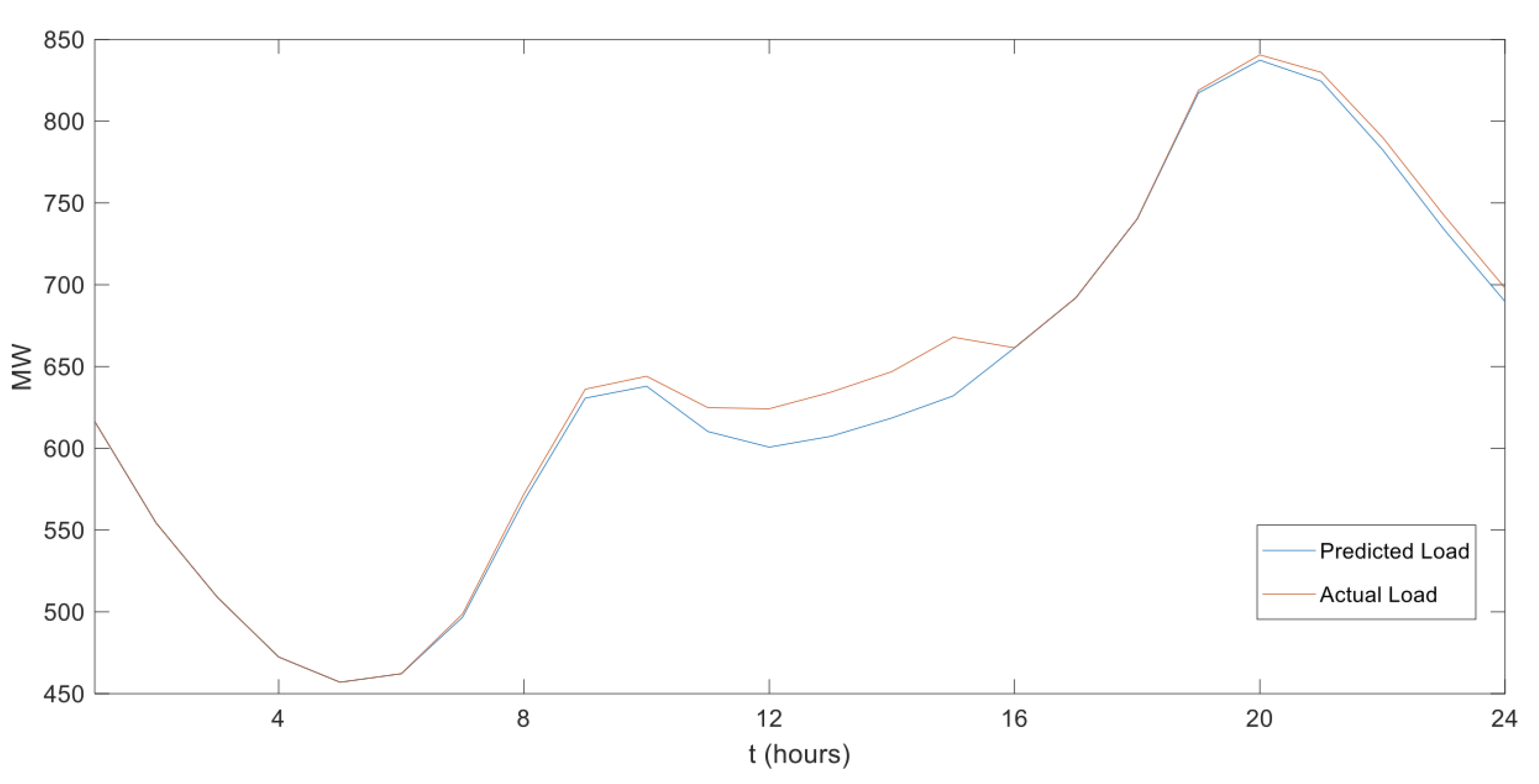
We provide the realization of our proposed solution to an energy-intensive winter day in Figure 14. In this case, one can observe how the negative temperature deviations between 10:00 and 16:00 affect the hourly-load forecast. Considering that $E=P·t$, this deviation corresponds to a daily power of 146.867 MWh or 35.864 MW instant power equivalent in the worst case. To recover this imbalance, a spinning reserve of up to 4.67% would be adequate if planned ahead.

Finally, we depict similar configurations for the more mitigated load curves in spring and autumn, together with the most energy-intensive day in summer, in Figure 15. For completeness sake, we list the comparative results with respect to the achieved SR capacity per month in

Table 1. Spinning reserve comparisons pertaining our proposed solution and robust alternatives.

Month	Load Demand (GWh)	Robust Formulation (GWh)	Real-Time Solution (GWh)
January	448.06	22.4	2.98
February	404.7	20.24	2.69
March	278.99	13.95	8.5
April	288.29	14.42	8.79
May	285.97	14.3	8.58
June	498.21	24.91	13.86
July	514.82	25.74	14.32
August	502.37	25.12	14.21
September	304.39	15.22	15.1
October	314.54	15.73	15.61
November	312.0	15.6	15.48
December	444.02	22.2	2.76

, considering the real-time weather impact and overall performance of our load forecasting model.

5. Conclusions

The continuous increase in the renewable energy contribution deteriorates the flexibility and stability of modern power systems calling for bulk spinning reserve margins. In this work, we proposed a dynamical forecaster to ameliorate the expensive requirements of spinning reserves based on real-time updates. Utilizing neural networks, we trained artificial models to forecast the load ahead with great accuracy, based on critical predictors and without using any model development structure to individuate and select the appropriate input parameters. Instead, we exploited eight predictors and distinguished them into constant and variable inputs by making use of a model predictive control. Apart from the most actively used data for historical load, seasonality and human activity, we also considered relative humidity as one of our main variable inputs. We performed real-time applications with the aid of a model predictive control, developed to update the recommendations intra-hourly and further correct the imposed deviations. Exploiting actual data regarding an isolated power system, the experimental results show that improvements exist in terms of decreased spinning reserve requirements to regulate the violated frequency. These findings strongly collaborate our claims and strengthen the arsenal of independent system operators with an effective tool for real-time load forecasting and total generation cost minimization.

As for future directions of research, we highlight the consolidation of more predictors correlated with renewable generation such as wind and solar. This way, a global forecaster could recommend the residual load target by making use of multi-input/multi-output neural networks. In addition, the fuel-dependent electricity prize may also take place as a real-time update, affecting both the human activity and hourly load demand.