1. Introduction
The growth of Renewable Energy Sources (RES) is expected to increase in the following years; among all the sources, the expansion is going to be led by solar photovoltaic (PV) at both the distributed and centralized levels [
1]. The penetration of non-programmable RES is posing great technical challenges to grid operators in terms of reliability and stability of the overall system [
2]. PV resource, in fact, is strongly dependent on meteorological conditions such as stochastic movements of clouds, fog, and other meteorological parameters that hinder solar radiation [
3,
4].
On a national level, a portfolio of different power plants with varying degrees of responsiveness is required to meet the continuously changing demands. However, while the aggregate load fluctuations vary within few percentage around the expected values, the power generation from plants exploiting RES presents larger and generally faster variations. For this reason, the shortness they can cause is usually faced with some “hot standby” spare capacity, which affects the overall efficiency of the system [
5]. For what concerns microgrids, the RES fluctuation is usually compensated by energy storage and backup technologies, which should be properly sized and coordinated, generally to increase efficiency, to reduce fuel consumption, or to wisely combine the two [
6,
7].
In this scenario, an accurate PV power forecast can greatly help operations; unit commitment; and, on a longer time horizon, sizing of available units, ultimately reducing investment costs [
8]. Selecting the more suitable prediction model in terms of accuracy is a big issue related to the forecasting topic. The available methodologies and their performances are highly affected by the selected time horizon and the task to be accomplished [
9,
10]. In fact, when PV modules are part of the generation units of a complex energy system, an integrated forecasting approach is useful to address several scopes. From the Energy Management System (EMS) point of view, a 24-h-ahead forecast is needed to initially perform strategic optimization of system management, with the goal of, for example, minimizing the operating cost, reducing the fuel consumption over the following 24 h, and properly managing and sizing the battery energy storage system (BESS) [
11,
12]. Approaching the operating time, additional refinements are useful to further correct the original forecast and to tune the dispatching schedule in the so-called intraday forecast [
13]. Eventually, during the operations, integration of the previous forecast for the following minutes is required for predictive power management [
14,
15].
The importance of short-term forecasting (in the range from 0 to 30 min), called
nowcasting, is growing due to regulatory issues [
16] and for optimal sizing and management of storage [
17]. In nowcasting, the main issue is related to identification of the sudden spikes and drops in PV power production. These fluctuations are mainly related to the presence of moving clouds, which hinder solar radiation. For this reason, most of the work found in the literature relies on the adoption of satellite images and whole sky images [
18,
19,
20,
21]. Other works rely on machine learning algorithms to serve the scope [
22].
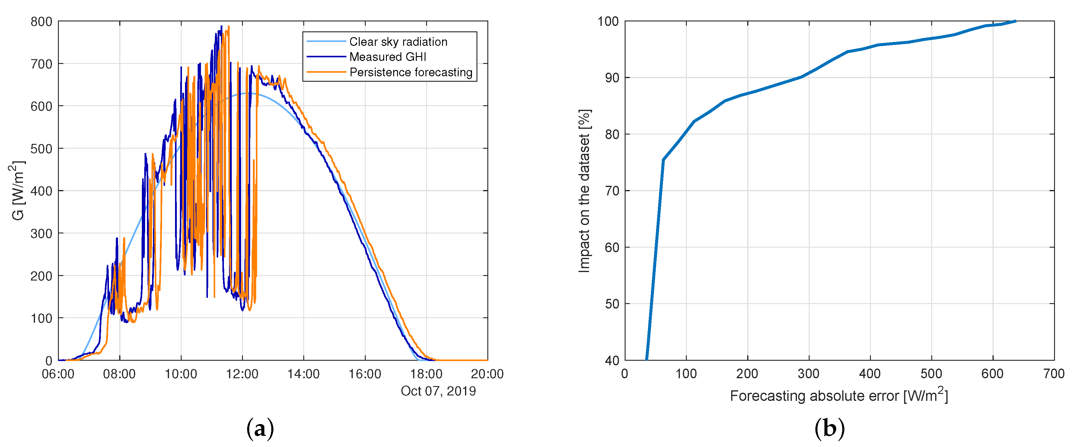
All the abovementioned approaches are usually compared with a benchmark, which is represented by the persistence. A persistence forecasting method consists of imposing the next value of the forecast parameter to be equal to the last measured one [
23]. In the very short term, this method achieves very good results, especially in stationary conditions, and presents the advantage of a negligible computational cost. Nevertheless, the validity of persistence loses effectiveness as the forecast horizon increases [
24].
The aim of this paper is to introduce, describe, and compare three different Sun identification techniques that can be applied to the nowcasting problem. This paper extends the preliminary analysis provided in [
25], providing more details on the motivations, deepening the investigation of the implemented techniques, and introducing some new numerical performance parameters that are used to test the implemented techniques against manual recognition.
The artificial neural network-based method-proposed technique is able to overcome the problem of finding the true optical distortion of the image acquisition system, often unknown in industrial applications. In fact, this method exploits the solar angle information that avoids, after the training process, complex and time-consuming image-processing operations.
This paper is structured as follows. In
Section 2, an analysis of sudden changes of the irradiance value that motivates the use of sky images for nowcasting is provided. Then, in
Section 3, the three different identification techniques are described in detail.
Section 4 shows a numerical and a qualitative comparison between the three approaches, and finally, in
Section 5 some conclusions are drawn.
3. Methods
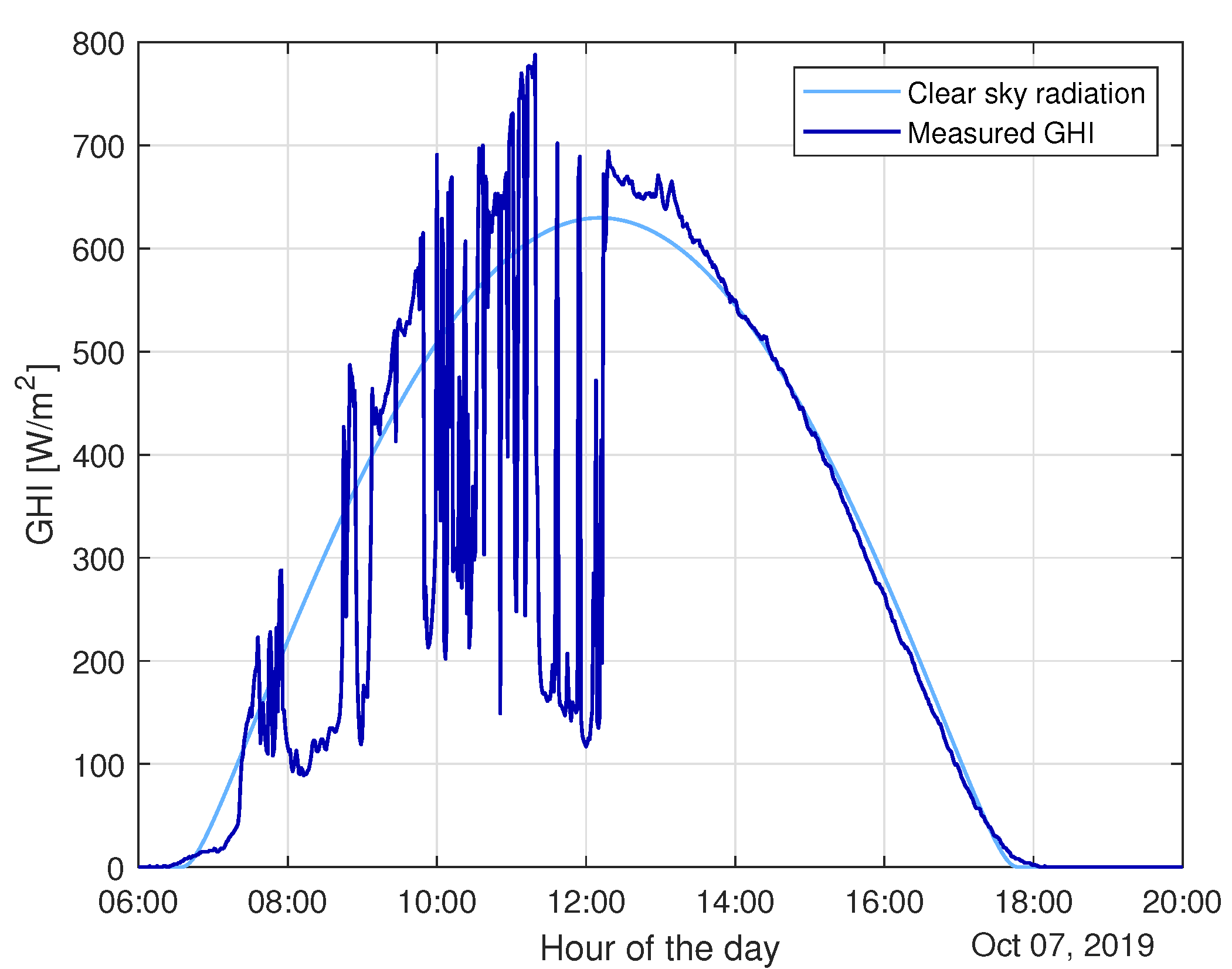
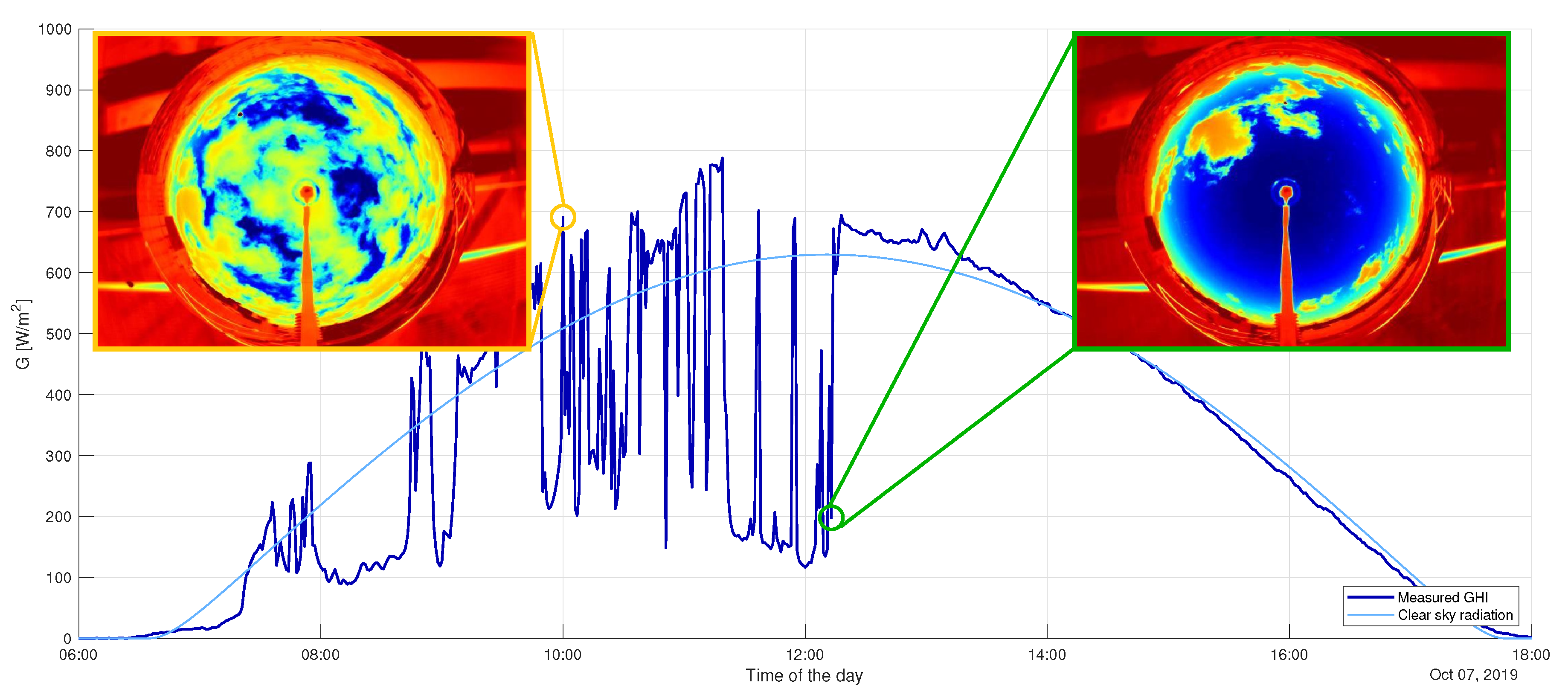
As said in the previous sections, PV nowcasting based on sky images is fundamental in spotting the solar behavior, such as spikes and drops in the measured irradiation that could hardly be identified through a purely statistic methodology.
In this paper, three different methods have been implemented, with increasing computational complexity and accuracy.
The first method exploiting information regarding the theoretical solar position provides the projection of the Sun on the image through a mathematical representation.
The second implemented method identifies the solar position by means of image processing. The overall accuracy of the method is higher than the previous one, though requiring more computational effort. The main drawback of this approach is the impossibility to identify the Sun when it is covered by clouds. Finally, the third method is based on Artificial Neural Networks (ANNs) that are able to infer the correlation between the theoretical solar angles and the solar position on the images; the strength of this approach is that, regardless of the weather conditions, it is able to provide the correct position of the Sun.
In the following sections, these methodologies are described in details.
3.1. Solar Angle-Based Identification
The first method relies on the solar angles that are commonly used to determine the Solar position in the sky.
The solar angles (azimuth
and elevation
) can be determined as function of the coordinates of the location and of the time of day. Their determination has been performed as presented in [
28] and implemented in [
29].
Once
and
have been computed, the approximated solar position on the image can be found applying the following trigonometrical relations:
where
L is the radius on the image and
is the two-dimensional vector for the central position on the image:
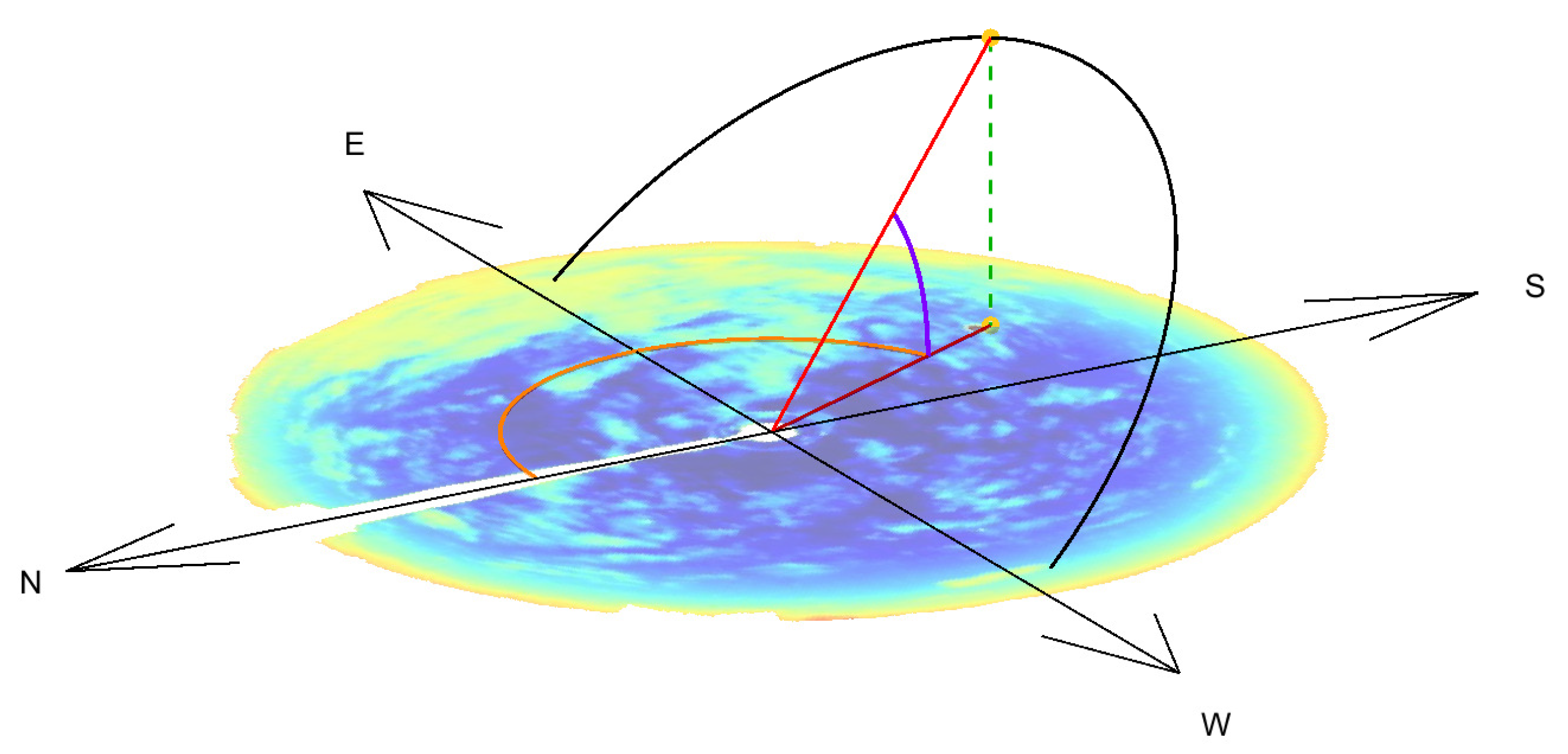
Figure 8 shows an example of the application of this technique. The black line represents the theoretical Sun trajectory in the sky, the upper yellow dot is the real position of the Sun, and the lower dot is its projection on the image; the central position is the point where the two red cross. The solar angles can be identified as follows: the orange arc represents the azimuth
(0° north, increasing towards east), and the purple one is the elevation
(0° representing the horizon, positive upwards).
This technique allows one to find the approximate solar position with simple trigonometric operations. Moreover, once the central position of the images is given, no further information regarding the images are needed. On the other hand, due to the optics and mirror surface distortion, unknown in the current work as well as in many industrial situations, it can only provide a rough estimation of the actual solar position.
The main advantage of this technique is hence the ease of determination of the solar position since it can be done without complex analyses or a historical dataset.
3.2. Image Processing-Based Identification
The second methodology is based on image processing algorithms, and it is capable of identifying the Sun by means of its shape and color.
The first step to be applied on the available images consists of a color threshold filtering, where the thresholds are imposed on all the pixels and color channels and their values are set for the specific case under study in order to identify the Sun. On the current images, in fact, the Sun appears as a dark dot.
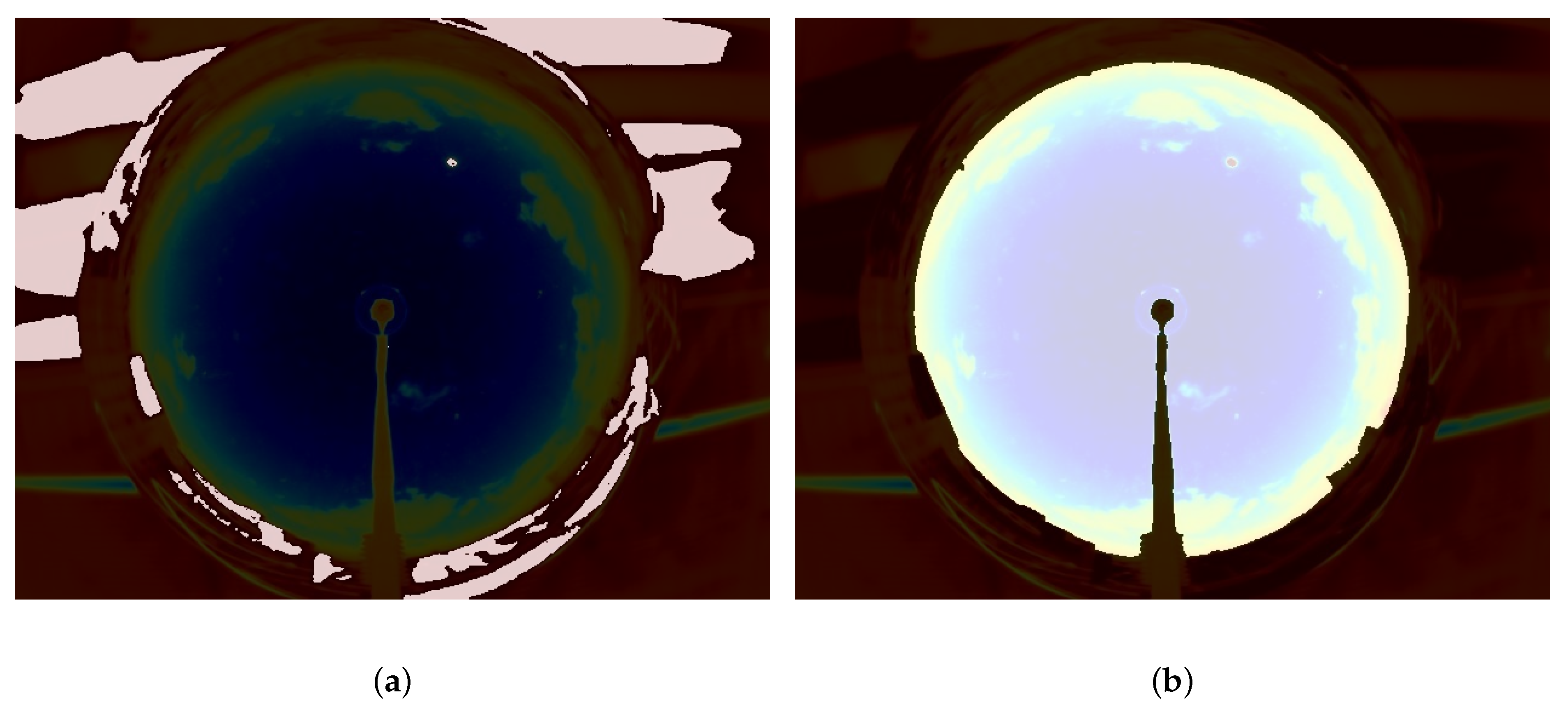
Figure 9a shows the color filtering result overlapped on a sample image: the whiter areas are the identified one as a candidate for the solar position, while the darker areas are discarded. As it is seen, there are large areas that belongs to the background and are not interesting to the scope. For this reason, thanks to the rigid geometry of the camera, it is possible to eliminate these areas applying a mask.
Figure 9b shows this mask: the central part (lighter) is the correct sky image.
Finally, the two combined filters (the first one constructed ad hoc for the frame under study,
Figure 9a, and the second one common for all images,
Figure 9b) are combined, returning some candidates eligible for the solution of the problem. Unfortunately, depending on the boundary effect due to the presence of the supporting pole for the camera and on the sky color variations, more than one identification can often be returned. To select the true identification, a position control is applied: information about the solar angles is exploited, and the search of possible locations of the Sun is reduced to an elliptical area surrounding of the position detected through the methodology explained in
Section 3.1. The choice of the elliptical shape is consequent to the fact that the error committed on radial distance from the central position
is greater than the error on the azimuth angle.
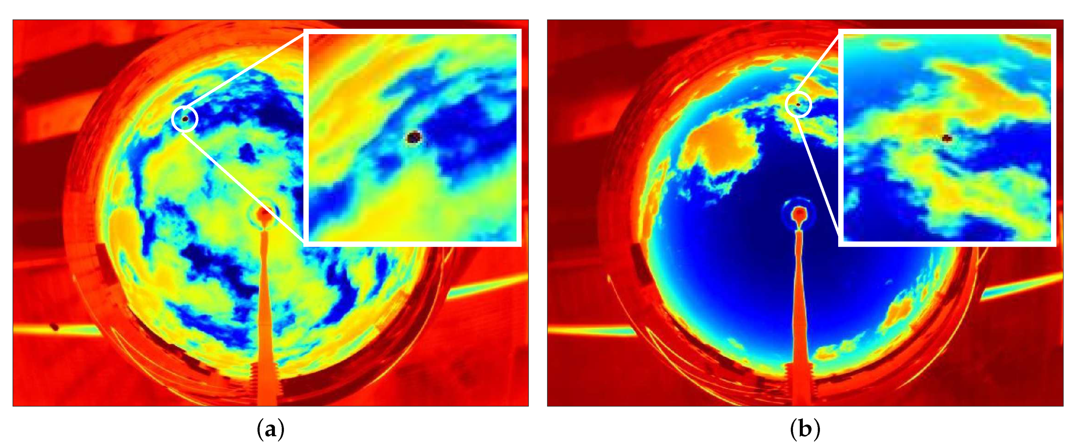
Figure 10 shows an example in which candidates were found. If the reduction of the search space were not applied, it would have not been possible to identify the correct solar position. On the other hand, the ellipse allows for proper identification of the desired solution, the only one in the elliptical shape.
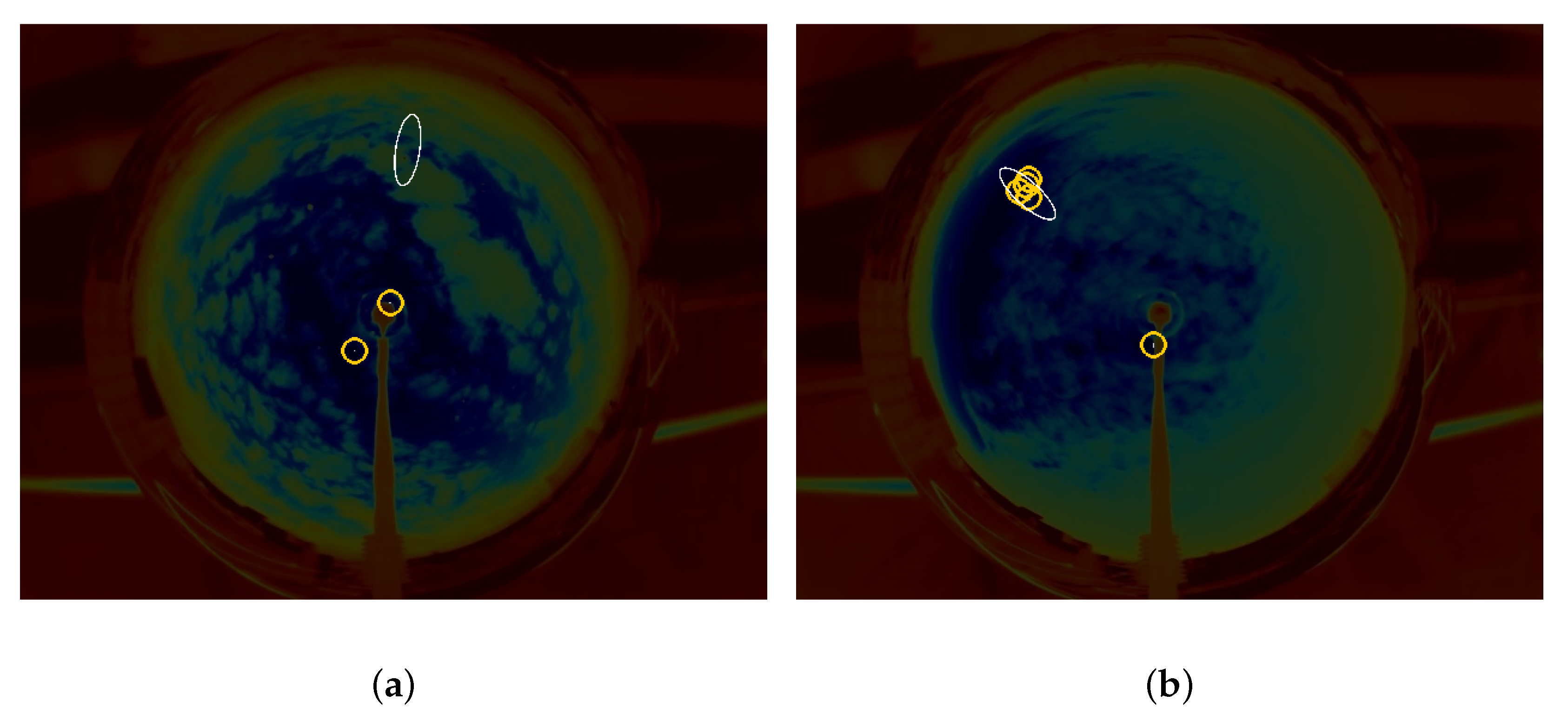
In some cases, such as the ones depicted in
Figure 11, two situations in which the algorithm returned multiple outcomes are presented. In
Figure 11a, two candidates are found, both of them false positives being outside the search space. In this case, the actual position of the Sun cannot be detected by the algorithm because it is hidden behind the clouds.
The opposite situation shown in
Figure 11b, typical of rainy days, represents multiple candidates found in the ellipse. Due to the impossibility of detecting the real position and in order to adopt a conservative approach, no Sun position is detected here.
Even if it can lead to some errors, this method is generally very accurate and the computational time required to process the images is quite limited.
The main drawback of this technique is related to the impossibility of finding the Sun when it is covered by clouds: this technique, in fact, is conservative and provides the Sun position only when the estimation satisfies the accuracy conditions modelled by the set of filters shown before. This is an important drawback because cloudy days are very important conditions that cannot be excluded from the study.
3.3. ANN-Based Identification
The third methodology aims at overcoming all drawbacks of the previously analysed techniques, i.e., the solar angle-based and the image processing-based. In particular, this methodology exploits the capability of Artificial Neural Networks (ANNs) learning from historical data without information concerning the system.
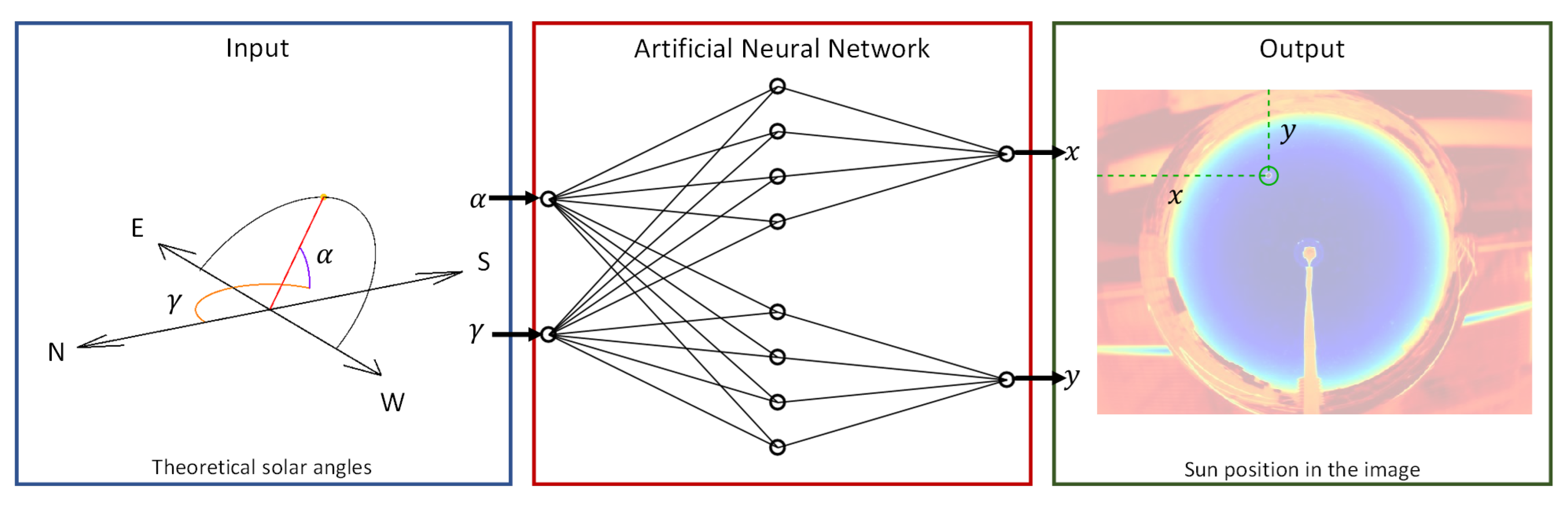
The ANN receives the solar angles () as input and returns the x- and y-coordinates of the Sun on the image as output. In this way, the neural network is able to eliminate the deformation introduced by the mirror and the optics of the camera.
Figure 12 shows the scheme of the neural network working process: the inputs of the network are solar angles (azimuth and the elevation), and the outputs are the x- and y-coordinates of the Sun on the image.
The aforementioned choice of inputs is not the only possible. Day and time could be used as well, but their adoption requires a higher number of historical data to let the network generalize the overall trend.
The implemented neural network has 10 hidden neurons for identification of both the x- and the y-coordinates. The training and test sets were obtained using an image dataset of 30 days. The outputs corresponding to the inputs are obtained through the image processing methodology explained above. Consequently, those samples where the image-processing fails at identifying the solar position were rejected and excluded from the training dataset. Finally, the overall number of available samples was equal to 9774.
The training process of the neural network was performed with 70% of the dataset, while 10% was used for validation. The remaining 20% was used for testing the system performance.
Due to the intrinsic stochasticity of the training process and in order to overcome possible local minima in the optimization process, 10 independent trials have been performed with a different subdivision of the training, validation, and test sets: the accuracy in all of them was very high, proving the robustness of the approach.
The main limitation of this methodology is related to the required training set: in fact, it is important to cover the entire range of possible solar angles because ANNs are very effective in interpolation but less accurate in extrapolation. However, the choice of the solar angles as the input reduces the number of required training days.
4. Results and Discussion
In the present section, the three above-described techniques are compared using the available dataset. In addition, a manual identification of the Sun position was conducted over the 30 available days to be used as a benchmark in the comparison.
In order to compare the performances of the solar identification techniques, three performance parameters were introduced. The first one, counting the number of revealed samples, provides an indication in terms of availability of the approach. In fact, it is desirable that the Sun position is identified in as many cases as possible. The second performance parameter, counting the wrong identifications with respect to manual analysis, provides information regarding the reliability. Two aspects were considered in this regard. Firstly, an identification is wrong if it is more than 3 pixels away from the manual one. Secondly, for the image processing-based technique, the number of false identifications is counted too (the Sun was not visible to the human eye, but it was detected by the algorithm). The choice regarding the number of pixels derives from the consideration that, through manual identification, the central position of the Sun was identified, and the solar disk can be greatly approximated by a circumference with radius equal to 3 pixels. Hence, all those outcomes inside this shape are considered correct.
Finally, the last performance parameter takes into account the time needed to identify the solar position for a whole day; for the neural network analysis, the training time (4.85 s) has not been taken into account because it is considered an initial overhead time, since it can be previously performed offline.
In
Table 1, the numerical comparison between the three techniques is given.
The number of identifications for the solar angle-based and neural-network recognitions corresponds to the total amount of samples in which the solar elevation is greater than zero. As for manual identification, this represents the number of frames in which the user was able to clearly identify the solar position. Finally, the number of samples identified by the image-processing technique is related to the presence of cloud coverage or high color distortion in early morning or late afternoon. In fact, the entire image processing procedure and the related user-defined parameter are set as a trade-off to reduce the number of false identifications while, on the other hand, not penalize the number of detected samples. It was finally decided to set them in a conservative way, with the aim of containing the false positive, with the identification being further used in the ANN training process. With respect to manual recognition, the number of detected samples is 7.46% less.
As for identification accuracy, worth highlighting is the poor performance of the solar angle-based method. This can be explained considering that the actual mirror geometry is not known. For this reason, the projection of the Sun on the images is not well-described by the polar coordinates. More effort could be put in the mathematical description that could finally lead to greater accuracy, that though could hardly reach the image processing accuracy. This methodology, in fact, allows for identification of the Sun with an accuracy of 99.07%. Despite this, the image process suffers from wrong identification, that is, the false identification in those images where the Sun is not visible. This mainly happens during rainy days, when drops of water on the reflectance surface hinder recognition. In general, these phenomena do not highly impact the overall effectiveness of the method but can generate disturbance and noise in the dataset used for the ANN learning process and must not be ignored. The ANN-based methodology is finally the method that returns the higher accuracy.
For what the required time is concerned, image processing is slightly slower than all the other automatic identifications (7.7 s with respect to the other techniques that require less than a second), but all of them are much faster than manual recognition. Worth highlighting is that solar angles and ANN -based methodologies are not dependent on the real-time acquired images but rely on theoretical information computed a priori and are ultimately dependent on the location and time.
In
Figure 13, the distance in terms of pixels from manual identification is provided for the 3 methods. As it possible to see, the solar angle methodology provides a near constant distribution in the range 0 to 9 pixels. On the other hand, both the image processing and the neural network-based techniques are able to provide good approximation of the solar position, with most of the identifications in the range 0 to 1 pixel.
In
Table 2, the information is numerically expressed in terms of mean and standard deviation (
and
, respectively) of the error committed by the three presented methodologies. Worth highlighting are the results obtained for both the image processing and neural network-based techniques. The neural network, in fact, is able to provide the same degree of approximation and accuracy through proper generalization of the solar path on the images.
To further understand the above results, some images are presented and their results are explained.
Figure 14 shows the solar paths identified by the three methods in near-clear-sky conditions: the red line is the solar angle-based identification, the orange line is the image processing-based, and the green line is the neural network-based methodology. The ANN trajectory is taken as reference thanks to the accuracy shown with respect to manual identification. As it is possible to see, the solar-angle-based technique shows the lowest performance, especially at the beginning and at the end of the day, while the two other trajectories mostly overlap.
The image processing-based method has some holes in the early afternoon due to the presence of clouds, and it is less capable of finding the Sun position at sunrise and sunset. In fact, in these conditions, the solar position can hardly be identified due to deformation of the shape and of the colors induced by the mirror.
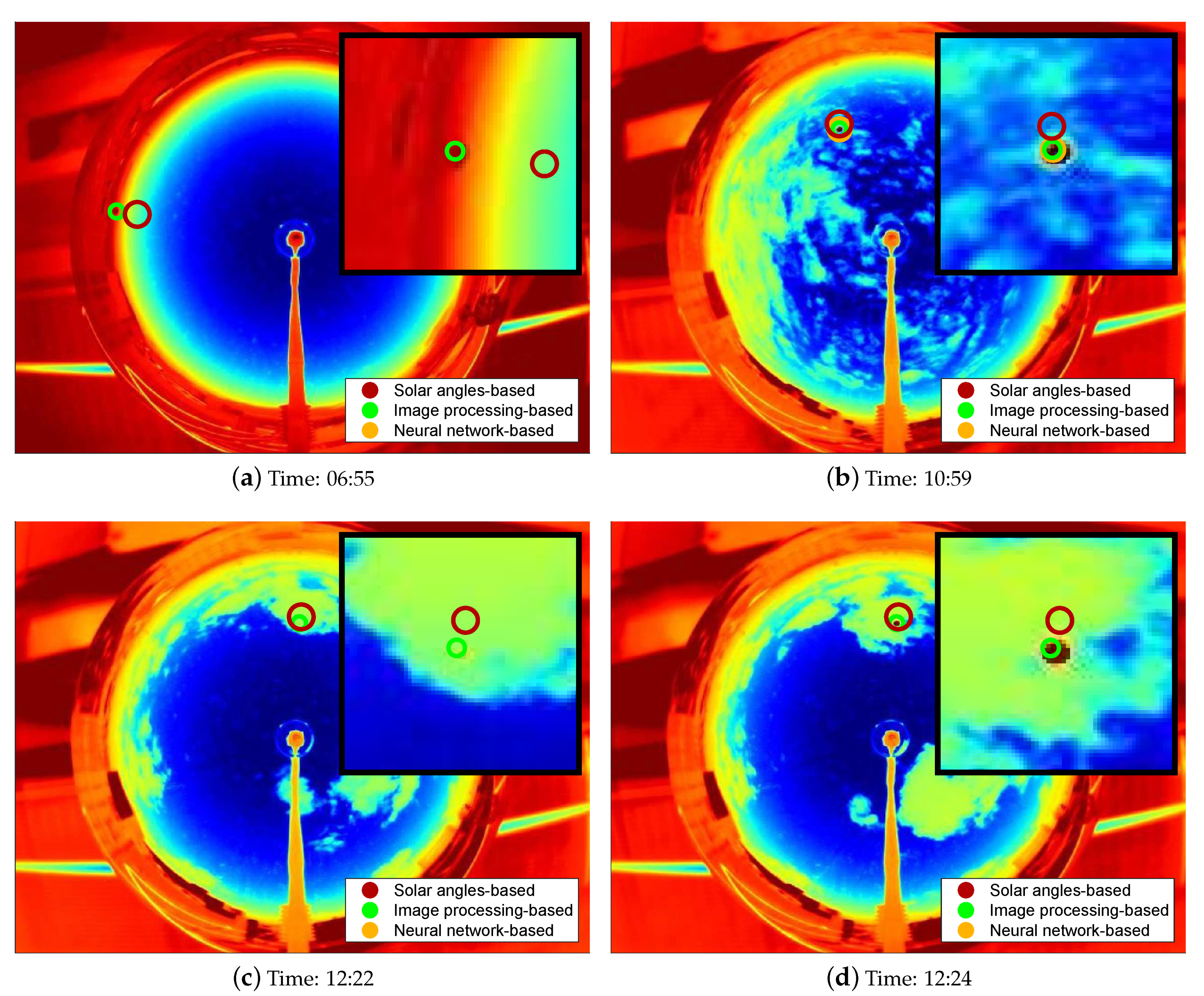
Figure 15 shows four different time instants of the same day. The time is synchronized with the Italian winter time (GMT + 1). For each image, the area around the position of the Sun has been magnified in the top right corner of each picture. In these images, the overall poor performance shown in
Table 1 of the solar angle-based method is confirmed: in fact, as it is possible to see, the red circles hardly overlap the other two in most of the images throughout the day.
Figure 15b shows that identification of the image processing-based method and of the neural network-based are almost coincident; this allows us to conclude that the learning process has been conducted properly and that the neural network learned the ability to infer the specific desired trend.
In
Figure 15a,d the solar position has been correctly identified by the neural network, while the image processing-based identification failed. In these images, in fact, the Sun is clearly evident in the zooms, but due to color distortion, image processing failed at identifying the position.
Finally,
Figure 15c shows a sample in which clouds cover the Sun. The neural network-based method can identify a candidate position analyzing the trajectories. The result is proven to be very close to the expected real Sun position.
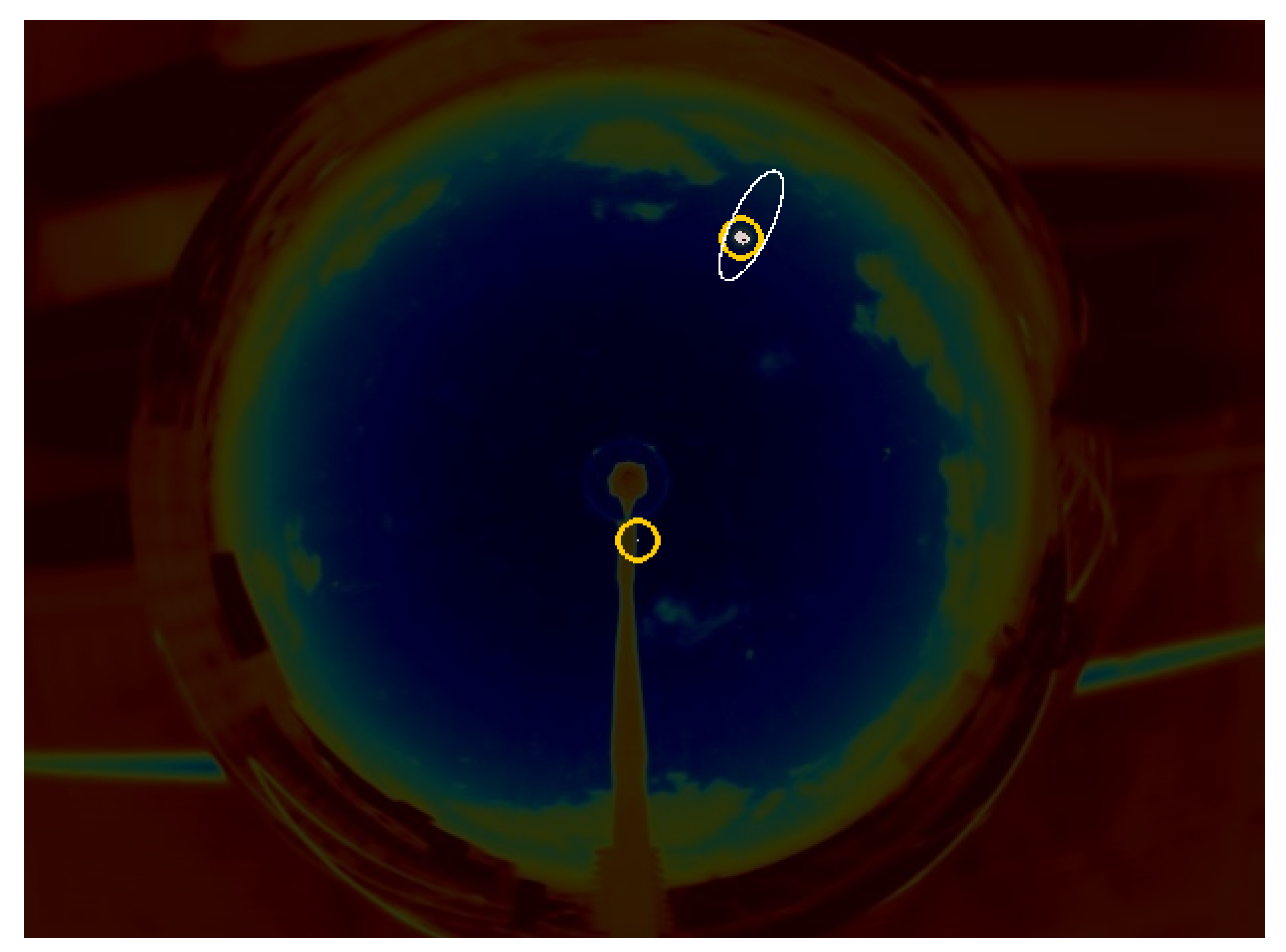
Figure 16 shows one of the rare cases in which identification by means of the image processing fails, providing an unreliable result. Analyzing the zoomed plot, it is possible to see that, while the neural network has been able to avoid this error, due to particular conditions such as the color distortion of the Sun and a spot of color saturation in the reduced elliptical shape, the image processing identified a single wrong accepted candidate. Despite those noises in the training dataset, the ANN learning process was able to mitigate their presence without compromising the overall prediction ability. This ability must be further examined by increasing the training dataset to a larger number of days.
5. Conclusions
In this paper, three different techniques aiming at identifying the solar position in whole-sky images were proposed, described, and compared. The implemented approaches were specifically set and tailored in order to serve the scope of providing a first step towards the definition of a novel methodology to perform very short-term PV power forecast, namely, nowcasting.
The first method relies on the theoretical solar position in the sky and was described in terms of the solar azimuth and elevation ( and , respectively). The projection of the theoretical position on the images was affected by approximation due to the partially unknown deformation introduced by the reflection and acquisition system. The second methodology performed identification of the Sun through an image processing algorithm exploiting the chromatic difference existing in the images among the sky, the Sun, and the surroundings. Finally, the third approach used information obtained through the first two methodologies to train an artificial neural network.
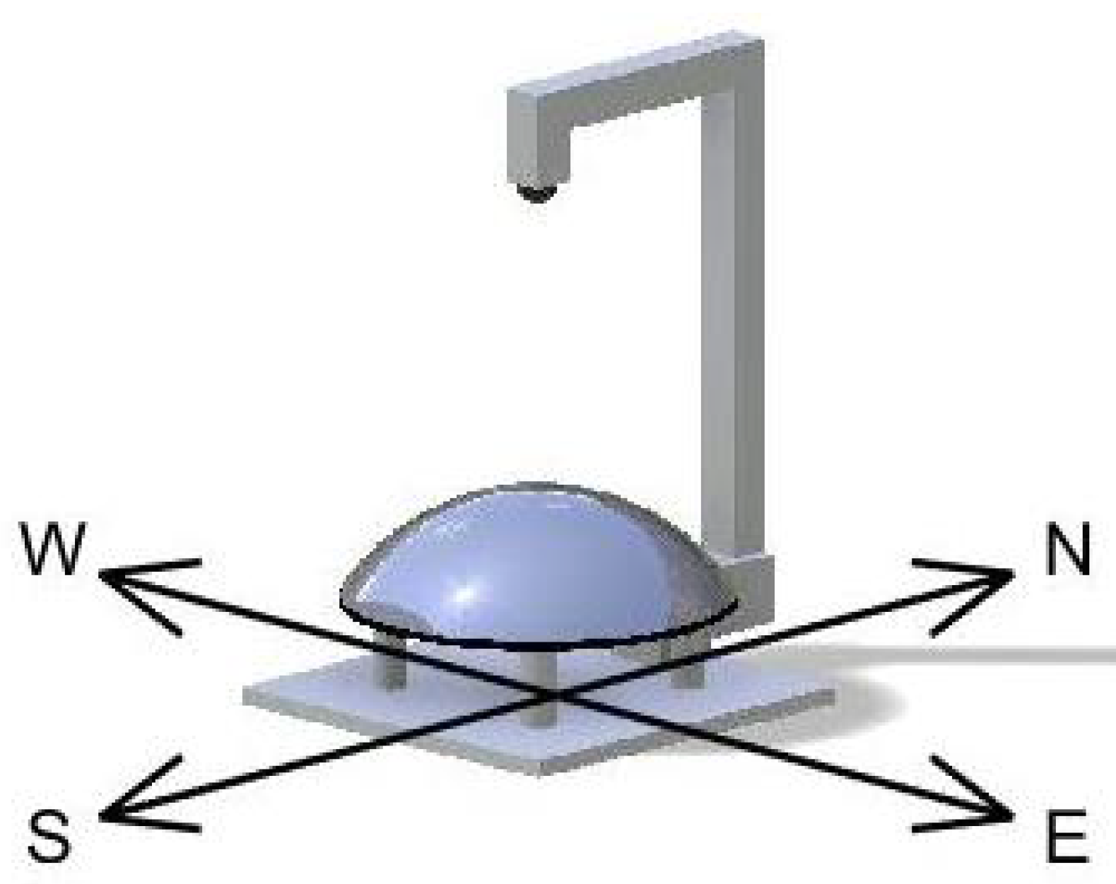
These proposed techniques were tested using real images obtained with a camera installed at SolarTechLab at Politecnico di Milano, Italy. They were compared in terms of reliability, accuracy, and computational load.
The overall best performances are obtained through the adoption of the ANN-based technique that, thanks to its generalization capability, is able to accurately infer the solar position in a wide spectrum of conditions: in fact, the error committed by this methodology is 0.01%, while the image processing-based method is above 3%.


