Photovoltaic Output Power Estimation and Baseline Prediction Approach for a Residential Distribution Network with Behind-the-Meter Systems

Abstract

Considering that most of the photovoltaic (PV) data are behind-the-meter (BTM), there is a great challenge to implement effective demand response projects and make a precise customer baseline (CBL) prediction. To solve the problem, this paper proposes a data-driven PV output power estimation approach using only net load data, temperature data, and solar irradiation data. We first obtain the relationship between delta actual load and delta temperature by calculating the delta net load from matching the net load of irradiation for an approximate day with the least squares method. Then we match and make a difference of the net load with similar electricity consumption behavior to establish the relationship between delta PV output power and delta irradiation. Finally, we get the PV output power and implement PV-load decoupling by modifying the relationship between delta PV and delta irradiation. The case studies verify the effectiveness of the approach and it provides an important reference to perform PV-load decoupling and CBL prediction in a residential distribution network with BTM PV systems.

1. Introduction

1.1. Background and Motivation

As the disadvantages of fossil fuel power generation become increasingly prominent, renewable energy generation is developing rapidly, especially photovoltaic (PV) generation [1,2,3]. The installed power capacity of renewable energy generation grew more than 200 GW, which is mostly PV generation in 2019 [4,5]. However, because of the intermittency and uncertainty of PV, the high penetration of PV could bring great challenges to the power grid, such as power distribution system planning and operation [6,7,8,9], load demand forecasting [10,11,12], hybrid energy system configuration [13,14], and PV power forecasting [15,16].

Demand response (DR) [17,18,19] is an effective method to improve the reliability and flexibility of the power distribution system [20,21,22]. In order to incent customers to participate in the DR program, the DR aggregators need to make decisions based on the customer baseline (CBL). Therefore, it is vital to predict the CBL accurately [23]. However, in a residential distribution network, the distributed PV owned by customers generally is located behind-the-meter (BTM) [24], which measures the net load and denotes actual electricity load minus PV power generation. Hence, the distributed PV generation, such as rooftop PV, makes it difficult to predict CBL with net load [25] due to the volatility of PV and load.

To solve the above issues, it is necessary to decouple the PV generation and electricity consumption load from net load data. The well-known method is to install additional meters to specifically monitor each PV for operators; however, it is infeasible as a result of high extra cost and privacy issues. Consequently, for a residential distribution network with BTM PV systems, the innovative approach to decouple PV-load and predict CBL from net load data is developed in this paper.

1.2. Literature Review

In recent years, there has been a large amount of literature on BTM PV, which involves BTM PV detection and capacity estimation [24,26], and BTM PV output power prediction [27,28], etc. In the meantime, it has been a heated research topic for PV-load decoupling and CBL forecasting. One of the common approaches is the PV physical model [29,30], established to simulate and disaggregate PV generation power; however, the detailed PV panel parameters (such as the size, material, azimuth, and tilt) and meteorological information including temperature and solar irradiation need to be known. The authors of [31] realized PV-load decoupling and PV parameters estimating through combining an iterative method with models including the PV physical model with the load estimation model. However, its performance particularly depends on the accuracy of the physical model. Fortunately, a variety of advanced measurement facilities have appeared in the power grid with the development of information technology, e.g., supervisory control and data acquisition (SCADA) and smart meters, etc. It has spawned the other approach (a data-driven approach), which has been investigated by some researchers to decouple PV output power from net load data.

The net load measured by smart meters was used to estimate the individual distributed PV’s capacity and generation power in [15] through a support vector regression model. Based on the hybrid data dimension reduction method and mapping function, the authors of [32] provided a data-driven method to predict BTM PV generation power. However, they need to meter the output power of a small amount of BTM PV output power, which is assumed to have the similar characteristics as the estimated BTM PV. In [33], the unsupervised method disaggregating PV was proposed, considering customers’ similar electricity consumption behavior with and without PV. Then, the authors in [34] further developed a disaggregation model to decouple PV-load considering a battery energy storage system (BESS). Nevertheless, the authors of [35] showed that it is different for the user with PV and without PV to consume electricity. To avoid these issues, considering both the PV output power and the harmonic current injected by the inverter of PV, the method was carried out in [36] to calculate the PV generation power. However, this method may not be appropriate when some PV installed without permission are included in the power distribution system.

In addition, the baseline (BL) prediction has been studied in some works. In [37], an improved support vector regression model with the ambient temperature of two hours before a DR event as input variables was implemented to predict the office building BL. The authors of [38] studied the CBL impacts on the profit of the company and customers through obtaining the CBL prediction of residential customers, and building the cost and profit function. To address the non-synchronous matching issues in the previous study, the authors in [39] proposed a clustering-based method to build a prediction model considered only on past DR daily load data instead of non-DR daily load data. The authors of [40] proposed a two-stage adaptive BL prediction method that combined the self-organizing map and k-means clustering methods to identify days similar to the tested day under DR events. Considering that determined BL prediction cannot reflect the users’ complex electricity consumption behavior, in [41] the authors proposed a probabilistic BL prediction model based on Gaussian process regression. In [42], customers are selected randomly to form a control group to predict the CBL.

Reviewing the above articles, most CBL predictions were for users who had not installed a distributed PV system. However, considering the impact of BTM PV, all separated PV output power information in the residential distribution network is unknown except for the net load data and meteorology data, which will greatly affect the final prediction accuracy.

To address the above issues in this paper, based on the nearest neighbor algorithm and artificial neural network method, a PV-load decoupling and CBL prediction approach is proposed for a residential power distribution system with BTM PV. The main contributions of this paper are as below:

• The net load is decoupled from PV output power and actual load precisely;
• To correct the deviation of the matched net load data, the relationship between PV output power and the solar irradiance, and the relationship between actual load and the temperature, are discovered and further formulated;
• The CBL is predicted based on the PV-load decoupling.

This paper is organized as follows. Section 2 introduces the problem formulation. The methods are provided in Section 3, including the data set division, the electricity consumption sensitivity analysis, PV output power sensitivity analysis, and baseline prediction. In Section 4, the case studies are shown. Finally, the conclusions are given in Section 5.

2. Problem Formulation

In the residential distribution network with BTM PV, both PV output power and actual load are concealed in the net load. It brings a huge challenge for operators to make some decisions including optimal power dispatching and BL prediction.

2.1. PV Output Decoupling

Same as the customer net load, the aggregated net load is composed of the aggregated actual load and aggregated PV output power. Let $D=\left\{d|1,2,\dots ,D_D\right\}$ be a set of day record and $T=\left\{t|1,2,\dots ,T_T\right\}$ be a set of timestamp, then the aggregated net load on time t day d can be formulated as follows:

$$P_{nl}(d,t)=P_{ac}(d,t)-P_{PV}(d,t),\forall d\in D,\forall t\in T$$

(1)

where $P_{nl}(d,t)$, $P_{ac}(d,t)$, and $P_{PV}(d,t)$ are the aggregated net load, aggregated actual load, and aggregated PV output power, respectively. Figure 1 gives an example for the composition of net load.

Considering that the roof solar PV systems are usually invisible for the aggregator, and in most cases, the small scale distributed PV systems (less than 10 kW) are not set up with a separated PV output power meter [24], it is a big challenge to obtain the pure PV output power without the relevant monitoring information. Therefore, the purpose of the study is to acquire the decomposed PV output power by historical load data, solar irradiation data, and temperature data.

Unlike industrial load, temperature is the main impact factor for residential load consumption behavior [43]. As for the magnitude of PV output, the solar irradiation received by the PV panel plays a decisive role [44]. Based on the above-mentioned characteristics of user electricity consumption and PV output power, this paper considers the sensitivity of actual load to temperature to correct the difference in actual load due to temperature in net load on different days, and then the solar irradiation and PV power relationship is obtained.

2.2. CBL Prediction

For users who have not installed distributed PV equipment, relatively few factors can affect the CBL prediction. The error of the CBL prediction mainly comes from the diversity of the electricity consumption behavior of aggregated users under different environmental conditions [38]. However, for the users with PV systems, the uncertainty of PV output power should also be taken into account. To reduce the error of forecasting the CBL when only net load is available, in this paper, the CBL of actual load is predicted initially based on the PV decomposition technology, and then combined with the PV output power to improve the CBL prediction results of aggregated users equipped with distributed PV equipment.

3. Methods

3.1. Data Set Division

Due to the large differences in solar irradiation and temperature amplitude in different seasons, it leads to different electricity consumption patterns and changes in PV output power. The data set is divided into four categories according to local seasonal conditions. The detailed division time of four categories are shown in

Table 1. Division time of four categories.

Season	Label	Duration
Spring	1	Early September to end of October
Summer	2	Early November to end of March
Autumn	3	Early April to end of May
Winter	4	Early June to end of August

.

Since the PV equipment does not generate electricity before sunrise and after sunset, a period $\tau =\{t_{rise},t_{rise}+1,\dots ,t_{set}\}$, $\tau \in T$ is set to indicate the time containing solar irradiation, where $t_{rise}$ and $t_{set}$ represent the time of sunrise and time of sunset, respectively. The net load data of each season is further divided into the part that contains PV power, named $P_{nl1}(s,d,t)$, and the part that does not contain PV power, named $P_{nl2}(s,d,t)$, where $s\in 1,2,3,4$, represents the label of seasons.

3.2. Load Consumption Sensitivity Analysis

3.2.1. Correlation between Electricity Consumption and Temperature

Aggregated consumers have different electricity consumption habits in different seasons, and the difference in electricity consumption behavior is largely driven by temperature. In order to reflect the degree of correlation between temperature and consumer electricity consumption, a statistical method called Pearson’s correlation coefficient [41] is used to measure the strength of the relationship between the two variables, as shown in Equation (2).

$$r\left(T_{m,av}\left(d\right),P_{ac,av}\left(d\right)\right)=\frac{{\displaystyle \sum _{d=1}^H\left(T_{m,av}\left(d\right)-{\overline{T}}_{m,av}\right)\left(P_{ac,av}\left(d\right)-{\overline{P}}_{ac,av}\right)}}{\sqrt{{{\displaystyle \sum _{d=1}^H\left(T_{m,av}\left(d\right)-{\overline{T}}_{m,av}\right)}}^2}\sqrt{{{\displaystyle \sum _{d=1}^H\left(P_{ac,av}\left(d\right)-{\overline{P}}_{ac,av}\right)}}^2}}$$

(2)

where $T_{m,av}$ and $P_{ac,av}$ represent the average temperature and average actual load, and ${\overline{T}}_{m,av}$ and ${\overline{P}}_{ac,av}$ represent the average value of T days average daily temperature and average actual load. The absolute values of Pearson’s correlation coefficient are less than or equal to 1. The closer the $r$ value is to 1 or −1, the stronger the positive or negative correlation between the two calculated variables. Conversely, the closer the $r$ value is to 0, the weaker the correlation between the calculated two variables.

3.2.2. Electricity Consumption Sensitivity Model

Although temperature is the main factor that affects actual load, it is almost impossible to get the numerical relationship between temperature and actual load, because actual load consumption is invisible in the considered scenario. What is certain is that the PV output power is similar when the solar irradiation is the same or very similar [26,27] at the same time in the same season. Thus, if we can find a suitable match of pairs of similar or consistent solar irradiation dates and record them, and further make a difference to the corresponding net load data from the recorded date, we can eliminate the impact of PV output data as much as possible and get the actual load difference as formulated by the following equation:

$$\begin{array}{l}{P}_{nl1}(s,d^i,t)-P_{nl1}(s,d^j,t)\approx P_{ac1}(s,d^i,t)-P_{ac1}(s,d^j,t)\\ \hspace{1em}\hspace{1em}s.t.\hspace{0.17em}R(s,d^i,t)\approx R(s,d^j,t)\end{array}$$

(3)

where $R$ denotes the solar irradiation, and $P_{ac1}$ denotes the actual load during the time period with solar irradiation. Since it is almost impossible to find a completely consistent daily PV curve pairing, we choose to search for a match at each time $t\in \tau$. Considering that for a single point in time, the approximate date of illumination is generally more than one, and to ensure the number of matching samples, for each time t, we use the absolute difference between two points as the evaluation criterion of similarity and select $h$ dates with the most similar solar irradiation data to match. With $∆R_{rad}^h\left(d^i,t\right)$ denoting the set of solar irradiance difference between day $d^i$ and another day with similar solar irradiance, $\left|∆R\left(d_{rad}^{i,h},t\right)\right|$ is the absolute difference values between the solar irradiation of day i and the solar irradiation of its hth closest day, and $I_{rad}^h\left(d^i,t\right)$ is the corresponding recording set of the date of solar irradiation similarity match. Their relationship could be given as follows:

$$\{\begin{array}{l}∆R_{rad}^h\left(d^i,t\right)=\left\{\left|∆R\left(d_{rad}^{i,1},t\right)\right|,\left|∆R\left(d_{rad}^{i,2},t\right)\right|,\dots ,\left|∆R\left(d_{rad}^{i,h},t\right)\right|\right\}\\ ∆R\left(d_{rad}^{i,j},t\right)=R\left(s,d^i,t\right)-R\left(s,d^j,t\right)\end{array}$$

(4)

$$I_{rad}^h\left(d^i,t\right)=\left\{d_{rad}^{i,1},d_{rad}^{i,2},\dots d_{rad}^{i,h}\right\}$$

(5)

The delta temperature set $∆T_{m,rad}^h\left(d^i,t\right)$ and approximate delta actual load set $∆P_{ac,rad}^{h\ast }\left(d^i,t\right)$ according to the date match $I_{rad}^h\left(d^i,t\right)$ can be calculated by Equations (6) and (7), respectively, according to the data match in Equation (5).

$$\{\begin{array}{l}∆T_{m,rad}^h\left(d^i,t\right)=\left\{∆T_m\left(d_{rad}^{i,1},t\right),∆T_m\left(d_{rad}^{i,2},t\right),\dots ,∆T_m\left(d_{rad}^{i,h},t\right)\right\}\hfill \\ ∆T_m\left(d_{rad}^{i,h},t\right)=T_m\left(d_{rad}^i,t\right)-T_m\left(d_{rad}^h,t\right)\hfill \end{array},t\in \tau ,i\ne h$$

(6)

$$\{\begin{array}{l}∆P_{ac,rad}^{h\ast }\left(d^i,t\right)=\left\{∆P_{ac}^{*}\left(d_{rad}^{i,1},t\right),∆P_{ac}^{*}\left(d_{rad}^{i,2},t\right),\dots ,∆P_{ac}^{*}\left(d_{rad}^{i,h},t\right)\right\}\hfill \\ ∆P_{ac}^{*}\left(d_{rad}^{i,h},t\right)=P_{nl}\left(d_{rad}^i,t\right)-P_{nl}\left(d_{rad}^h,t\right)\hfill \end{array},t\in \tau ,i\ne h$$

(7)

where $∆T_m\left(d_{rad}^{i,h},t\right)$ represents the temperature difference between $T_m\left(d_{rad}^i,t\right)$ and $T_m\left(d_{rad}^h,t\right)$. $∆P_{ac}^{*}\left(d_{rad}^{i,h},t\right)$ is the approximate actual load difference between $P_{nl}\left(d_{rad}^i,t\right)$ and $P_{nl}\left(d_{rad}^h,t\right)$.

Given the delta temperature set and the approximate delta actual load set, the aim of this part is to perform a fit between these two sets of variables. From Section 3.2.1 we know that the temperature and actual load have a strong linear correlation. Especially in summer and winter, showing strong positive and negative correlations, respectively. Thus, we consider using a linear regression for curve fitting [45]. While taking into account that in the hypothesis when in the case of the same temperature situation, the actual load of the users should also be the same, that is to say when $∆T_m\left(d_{rad}^{i,h},t\right)$ equals to 0, $∆P_{ac}^{*}\left(d_{rad}^{i,h},t\right)$ also equals to 0. Therefore, the proportional function is selected as the fitting function and the least squares method is used to solve slope $k_{temp,ac}\left(t\right)$, which can be expressed in Equation (8).

$$\{\begin{array}{l}∆P_{ac,rad}^{h\ast }\left(d^i,t\right)=k_{temp,ac}\left(t\right)\times ∆T_{m,rad}^h\left(d^i,t\right)\hfill \\ k_{temp,ac}\left(t\right)=\frac{{\displaystyle \sum _{i=1}^{n_s}{\displaystyle \sum _h∆T_m\left(d_{rad}^{i,h},t\right)\times ∆P_{ac}^{*}\left(d_{rad}^{i,h},t\right)}}}{{\displaystyle \sum _{i=1}^{n_s}{\displaystyle \sum _k∆T_m{\left(d_{rad}^{i,h},t\right)}^2}}}\hfill \end{array}$$

(8)

where $n_s$ represents the total number of days in season s. Noting that each time $t\in \tau$ has a slope $k_{temp,ac}\left(t\right)$, hence there are $\left(t_s-t_r+1\right)$ slopes in total. Figure 2 shows the example of scatter plots of delta temperature and delta actual load at 17:00 in winter and summer and its corresponding linear fitting line.

3.3. PV Output Power Sensitivity Analysis

3.3.1. PV Output Power Sensitivity Model

Similar to the method mentioned in Section 3.2.2, if a similar actual load consumption behavior in two days is found, then we make a difference of net load of the corresponding days, and the interrelated approximated delta PV output power can be obtained. Even though the total actual load cannot be found, partial actual load can still be determined. Because of the absence of sunlight where the period in which PV outputs equals to zero, the net load is given as:

$$P_{nl2}(d^i,t)=P_{ac2}(d^i,t),t\in \overline{\tau },\tau \cup \overline{\tau }=T$$

(9)

where $\overline{\tau }$ is the complement of $\tau$.

Generally speaking, users’ electricity consumption behavior is continuous. Therefore, if the daily electricity consumption behavior in $t\in \overline{\tau }$ period is as similar as possible, the electricity consumption behavior in $t\in \overline{\tau }$ period is as similar as possible to a large extent. The k nearest neighbor (KNN) algorithm [46] is used to find the approximate $P_{nl2}$.

K nearest neighbor is one of the most simple and effective data mining algorithms. It is proposed based on similar sample points close to each other in space. The principle of the KNN classification algorithm is that if a sample to be classified has $k$ most similar (i.e., the nearest neighbors in the feature space) samples in the feature space, most of which belong to a certain category, the sample also belongs to this category. Therefore, when applying KNN to search for similar electricity consumption behavior curves, the similarity measure is performed on the feature space of each day $d^i$, and the first $k$ approximate samples are selected as the $k$ neighbors of $d^i$. The feature space of $d^i$ is $P_{nl}{}_2\left(d^i,t\right)$, $t\in \overline{\tau }$ and the similarity of feature space of $d^i$ and $d^j$ is assessed via Euclidean distance $\rho \left(d^{i,j}\right)$ using Equation (10).

$$\rho \left(d^{i,j}\right)=\sqrt{{\displaystyle \sum _{t\in \overline{\tau }}{\left(P_{nl}{}_2\left(d^i,t\right)-P_{nl}{}_2\left(d^j,t\right)\right)}^2}},i\ne j$$

(10)

The smaller the value of $\rho \left(d^{i,j}\right)$, the more similar the electricity consumption behavior in the two days (i.e., day i and j). Hence, we can also select $k$ dates with the most similar electricity consumption behaviors data to match. The dates recording set is as follows:

$$I_{beh}^k\left(d^i\right)=\left\{d_{beh}^{i,1},d_{beh}^{i,2},\dots d_{beh}^{i,k}\right\},i\ne k$$

(11)

where $d_{beh}^{i,k}$ is the recording date of electricity consumption behavior of kth nearest neighbor. Then we can make the following assumptions:

$$\begin{array}{l}{P}_{nl1}(d^i,t)-P_{nl1}(d^j,t)\approx P_{PV1}(d^j,t)-P_{PV1}(d^i,t)\\ \hspace{1em}\hspace{1em}s.t.\hspace{0.17em}\rho \left(d^{i,j}\right)\approx 0\end{array}$$

(12)

The delta solar irradiation set $∆R_{beh}^k\left(d^i,t\right)$ and approximate delta PV output power set $∆P_{PV,beh}^{k\ast }\left(d^i,t\right)$ can be calculated by Equations (13) and (14), according to the dates recording in Equations (11) and (12).

$$\{\begin{array}{l}∆R_{beh}^k\left(d^i,t\right)=\left\{∆R\left(d_{beh}^{i,1},t\right),∆R\left(d_{beh}^{i,2},t\right),\cdots ,∆R\left(d_{beh}^{i,k},t\right)\right\}\hfill \\ ∆R\left(d_{beh}^{i,k},t\right)=R\left(d_{beh}^i,t\right)-R\left(d_{beh}^k,t\right)\hfill \end{array}, t\in \tau ,i\ne k$$

(13)

$$\{\begin{array}{l}∆P_{PV,beh}^{k\ast }\left(d^i,t\right)=\left\{∆P_{PV}^{*}\left(d_{beh}^{i,1},t\right),∆P_{PV}^{*}\left(d_{beh}^{i,2},t\right),\dots ,∆P_{PV}^{*}\left(d_{beh}^{i,k},t\right)\right\}\hfill \\ ∆P_{PV}^{*}\left(d_{beh}^{i,k},t\right)=P_{nl}\left(d_{beh}^i,t\right)-P_{nl}\left(d_{beh}^k,t\right)\hfill \end{array},t\in \tau ,i\ne k$$

(14)

where $∆R\left(d_{beh}^{i,k},t\right)$ represents the solar irradiation difference between $R\left(d_{beh}^i,t\right)$ and $R\left(d_{beh}^k,t\right)$. $∆P_{PV}^{*}\left(d_{beh}^{i,k},t\right)$ is the approximate PV output power difference between $P_{nl}\left(d_{beh}^i,t\right)$ and $P_{nl}\left(d_{beh}^k,t\right)$.

Now we have the two sequences $∆R_{beh}^k\left(d^i,t\right)$ and $∆P_{PV,beh}^{k\ast }\left(d^i,t\right)$, the next step is to get the relationship between these two sequences. It is worth noting that, unlike the electricity consumption sensitivity model mentioned in Section 3.3.1, when the temperature is equal to 0, the electricity consumption is not necessarily 0. For this section, when the solar irradiation is equal to 0, the PV output is also 0. That is to say, through this characteristic, when we find the relationship between delta solar irradiation and approximate delta PV output power, we also find the relationship between solar irradiation and PV output power. The derivation process is formulated as:

$$\{\begin{array}{l}∆R\left(d_{beh}^{i,k},t\right)=R\left(d_{beh}^i,t\right)-R\left(d_{beh}^k,t\right)=Ra{d}_{amp}\left(t\right)-0\hfill \\ ∆P_{PV}^{*}\left(d_{beh}^{i,k},t\right)=P_{nl}\left(d_{beh}^i,t\right)-P_{nl}\left(d_{beh}^k,t\right)\approx -P_{PV}\left(d_{beh}^i,t\right)+P_{PV}\left(d_{beh}^k,t\right)=P{V}_{amp}\left(t\right)-0\hfill \\ ∆R\left(d_{beh}^{i,k},t\right)~∆P_{PV}^{*}\left(d_{beh}^{i,k},t\right)\Rightarrow Ra{d}_{amp}\left(t\right)~P{V}_{amp}\left(t\right)\hfill \end{array}$$

(15)

where $Ra{d}_{amp}\left(t\right)$ represents the equivalent solar irradiation amplitude of $∆R_{beh}^k\left(d^i,t\right)$, $P{V}_{amp}\left(t\right)$ represents the equivalent PV output power amplitude of $∆P_{PV}^{*}\left(d_{beh}^{i,k},t\right)$, and $~$ represents the symbol of derivation.

3.3.2. PV Output Power Sensitivity Model Based on Electricity Consumption Sensitivity Correction

The accuracy of decoupling the PV output power curve using the method in Section 3.3.1 depends largely on whether we can find the power consumption curves as similar as possible to match. However, due to actual conditions (insufficient historical data or similar electricity consumption behaviors that have not appeared in historical data), it is nearly impossible to find two completely consistent electrical behavior curves. Therefore, in most cases, there are large errors in the estimation of PV output curves according to the method in Section 3.3.1.

Our mentality is to choose two suitable dates to offset the actual consumption load $P_{ac}$ part of net load $P_{nl}$ as much as possible. However, the similarity of the matching curve in the $\tau$ period can only guarantee the similarity of the part of actual load of the matching curve pair in the $\overline{\tau }$ period to a certain extent. Therefore, we hope to make some corrections to modify the two curves to have more similar electricity consumption behavior during the $\overline{\tau }$ period. Although we cannot directly tell what the delta load $∆P_{ac}$ of the matched two-day curve is in the $\overline{\tau }$ period, we can gain insights about the temperature difference $∆T$ between the corresponding two days in the $\overline{\tau }$ period. In other words, through the relationship of Equation (8) obtained in Section 3.2.2, we can approximate the correction of actual load difference between the two matching curves $P_{cor}$ in Equation (16).

$$P_{cor}\left(d_{beh}^{i,k},t\right)=k_{temp,ac}\left(t\right)\times ∆T\left(d_{beh}^{i,k},t\right)$$

(16)

Then, Equation (15) can be rewritten as:

$$\{\begin{array}{l}∆R\left(d_{beh}^{i,k},t\right)=R\left(d_{beh}^i,t\right)-R\left(d_{beh}^k,t\right)=Ra{d}_{amp}\left(t\right)-0\hfill \\ \begin{array}{cc}∆P_{PV}^{*}{}^{\prime }\left(d_{beh}^{i,k},t\right)\hfill & =P_{nl}\left(d_{beh}^i,t\right)-P_{nl}\left(d_{beh}^k,t\right)-P_{cor}\left(d_{beh}^{i,k},t\right)\hfill \\ & \approx -P_{PV}\left(d_{beh}^i,t\right)+P_{PV}\left(d_{beh}^k,t\right)-P_{cor}\left(d_{beh}^{i,k},t\right)=P{V^{\prime }}_{amp}^{}\left(t\right)-0\hfill \end{array}\\ ∆R\left(d_{beh}^{i,k},t\right)~∆P_{PV}^{*}{}^{\prime }\left(d_{beh}^{i,k},t\right)\Rightarrow Ra{d}_{amp}\left(t\right)~P{V^{\prime }}_{amp}^{}\left(t\right)\hfill \end{array}$$

(17)

where $∆P_{PV}^{*}{}^{\prime }\left(d_{beh}^{i,k},t\right)$ represents the correction of $∆P_{PV}^{*}\left(d_{beh}^{i,k},t\right)$, and $P{V^{\prime }}_{amp}^{}\left(t\right)$ represents the equivalent PV output amplitude of $∆P_{PV}^{*}{}^{\prime }\left(d_{beh}^{i,k},t\right)$.

3.3.3. Evaluation Index of the PV Output Power Estimation

Mean absolute error (MAE) is used as the first evaluation indicator to calculate the accuracy of the decoupling results; the definition formula is as follows:

$$MA{E}_{PV}=\frac{1}{N}{\displaystyle \sum _{t\in \tau }\left|P_{est}\left(t\right)-P_{real}\left(t\right)\right|}$$

(18)

where $P_{est}\left(t\right)$ and $P_{real}\left(t\right)$ represent the estimated value and real value of the PV output power at time $t$, and $N$ represents the total time stamps during period $\tau$.

Considering the PV output power value is extremely small or zero during the periods of sunrise and sunset or under certain extreme weather conditions, it is therefore not suitable to use mean absolute percentage error (MAPE) as a judgment indicator. However, we still want to show the decomposition effect more intuitively, so the following formula is defined to reflect the relative error of the estimated daily PV output power:

$$RA{E}_{PV,daily}=\frac{{\displaystyle \sum _{t\in \tau }\left|P_{est}\left(t\right)-P_{real}\left(t\right)\right|}}{{\displaystyle \sum _{t\in \tau }{P}_{real}\left(t\right)}}$$

(19)

where $RA{E}_{PV,daily}$ represents the daily relative absolute error (RAE).

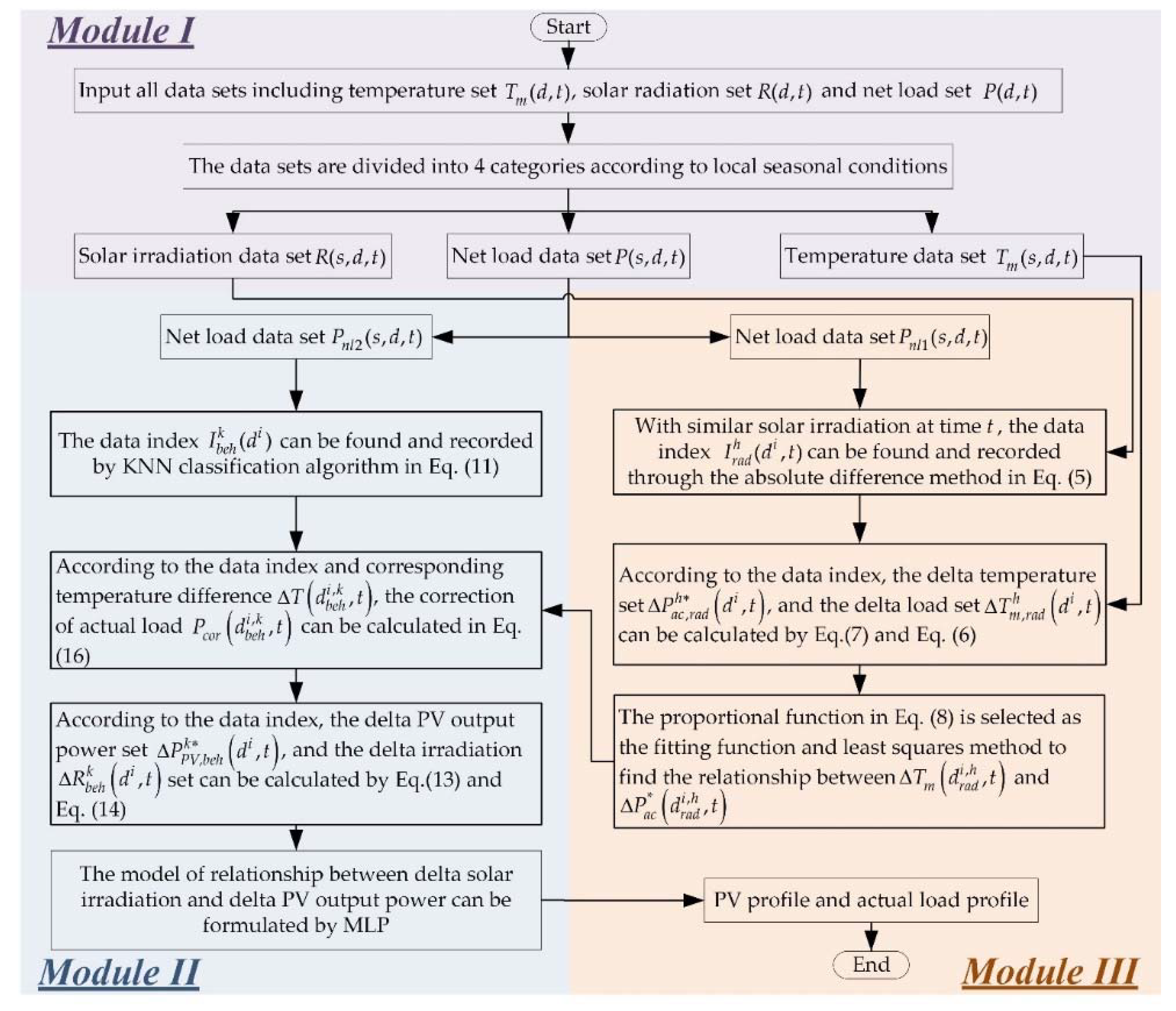
The decomposition process of PV output power from the net load proposed is shown in the following Figure 3.

3.4. CBL Prediction Model Construction

In this section, the decomposition technology of PV output power is applied to forecast the CBL of user groups equipped with distributed PV systems to improve the accuracy of the prediction results. Since the CBL prediction makes no difference from the situation without a distributed PV system during the period $\overline{\tau }$, the CBL prediction in this paper mainly focuses on the scenario of the period $\tau$. There are two methods for CBL prediction.

3.4.1. Direct Prediction Method

For the situation of PV output behind-the-meter, the CBL can only be predicted by the history net load of the non-DR event days. For CBL forecasting techniques, the most commonly used and effective method is the averaging algorithms and regression algorithms. The averaging algorithms mainly have the following three types, as given in

Table 2. Summary of the averaging methods.

Baseline Estimation Model	Definition
High $X$ of $Y$	The average load of the $X$ highest consumption days within those $Y$ non-DR days preceding the DR event days
Low $X$ of $Y$	The average load of the $X$ lowest consumption days within those $Y$ non-DR days preceding the DR event days
Mid $X$ of $Y$	The average load of the $X$ middle consumption days within those $Y$ non-DR days preceding the DR event days

.

In this paper, we also use multilayer perceptron (MLP) [47] and recurrent neural network (RNN) [48] as representatives of regression algorithms, and use historical net load data to forecast CBL.

From the definition of each average model and the characteristics of the regression algorithm, CBL of DR days can only be obtained through historical net load in the direct estimation method. This method may increase the forecast error due to the inability to consider the uncertainty of PV.

3.4.2. Prediction Method Based on PV Output Separation

Since we can peel off the PV output power through temperature and solar irradiation data, the actual load and PV output power on DR days can be predicted separately. The CBL prediction of the actual load part $P_{ac,BL}$ can be considered as the CBL prediction from the users that have not installed a distributed PV system. Then, we can get the final CBL prediction $P_{nl,BL}\left(t\right)$ by subtracting the part of separated PV output power $P_{PV,BL}\left(t\right)$; the equation is given as follows:

$$P_{nl,BL}\left(t\right)=P_{ac,BL}-P_{PV,BL}\left(t\right).$$

(20)

3.4.3. Evaluation Index of CBL Prediction

We evaluate the effect of CBL prediction methods from three perspectives (accuracy, bias, and variability). MAE is used for the evaluation of accuracy, which represents the absolute value of the difference between the true CBL and the predicted CBL. Bias is measured using the mean of the average error between the predicted CBL and the true CBL. Relative error ratio (RER) is used for the evaluation of variability, which represents a fraction of average load during the period $\tau$ [39].

4. Case Study

This section shows the effectiveness of the proposed PV output power curve decomposition and its application to CBL prediction.

4.1. Experimental Data Set and Platform Description

We used the load data set sourced from 300 randomly selected solar customers in Ausgrid’s electricity network area as the experimental data. The customers chosen had a full set of actual load data and PV output power data for the period from 1 July 2010 to 30 June 2011. In other words, we had intuitive and separate statistics of PV output power data to measure the accuracy of the proposed decomposition method. The temperature and solar irradiation data of the relevant area were from the website [49]. The resolution of the data sets are 48 points per day.

The CPU used in the experiment was an Intel(R) Core(TM) i5-6500 @ 3.20 GHz and the RAM was 8 GB. Python 3.7.7 was used for experimental simulation. The aggregated data was summed by 300 customers’ data. Timewise, 7:00–17:30 was set as the $\tau$ period. For the PV decomposition part of the experiment, the data of 1096 days in 3 years were used to derive the relationship between the solar irradiation and the PV output power. The total processing times of the method was 43.8 s, which meets the requirements of real-time PV output power estimation.

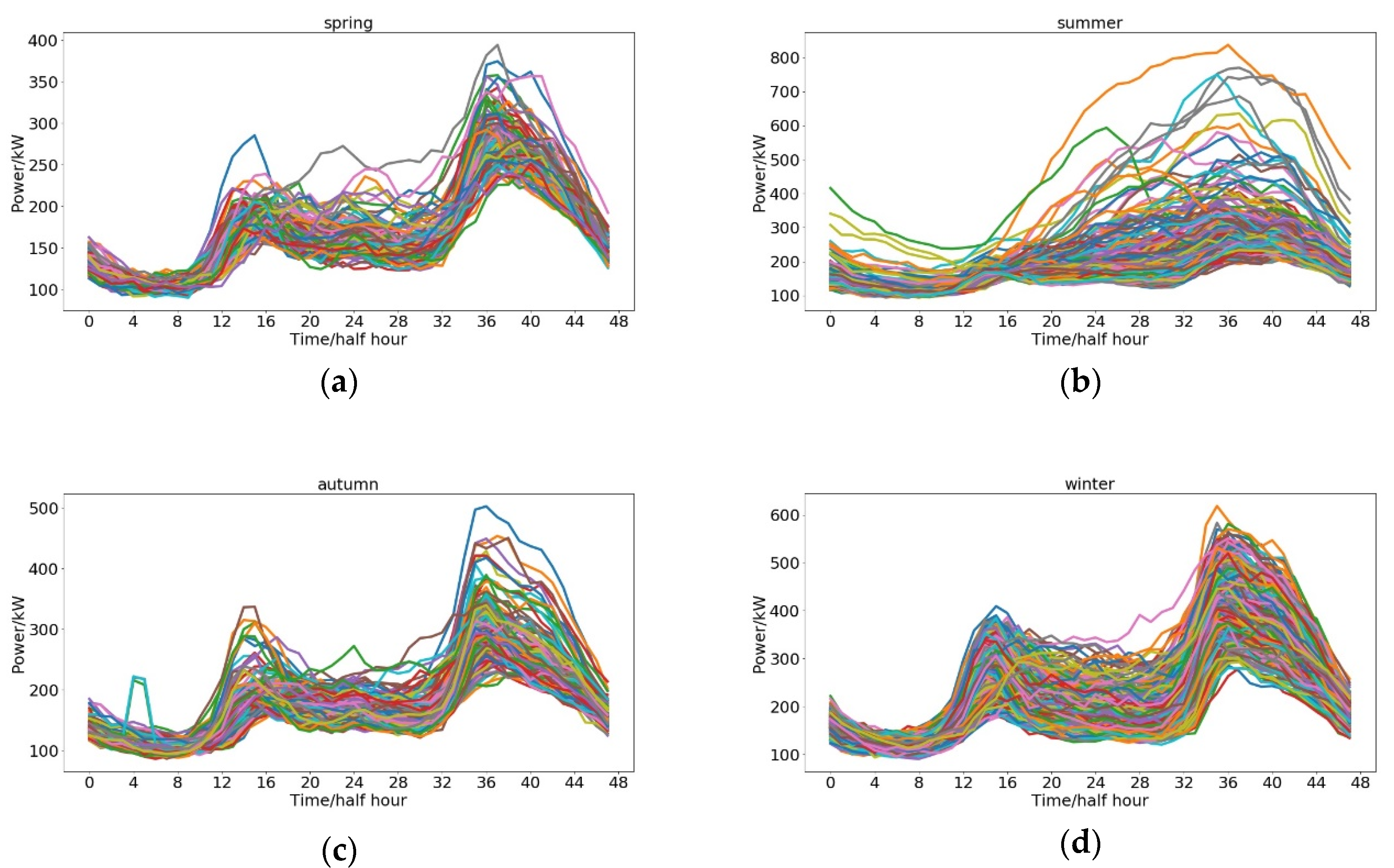
According to the season division rules in this paper, there are 98 days in spring, 460 days in summer, 169 days in autumn, and 369 days in winter. The clusters of actual load curves of four seasons are shown in Figure 4.

It can be seen from the figure that the actual load is relatively large due to the influence of air conditioning in summer and heating equipment in winter. For spring and autumn, the load has a similar shape. This is because the temperature in Australia in spring and autumn is similar, and the electricity consumption behavior of users is relatively consistent. Although the clusters of various seasons in the figure show that individual curves do not obey the group trends, one of the reasons could be due to extreme weather (cold wave and heat wave) in Australia. The division based on seasons can still effectively aggregate the actual load curves with the same electricity consumption pattern on the whole, which shows that clustering the net load based on different seasons is a good foundation for solving the temperature sensitivity of load consumption in the next step.

4.2. PV Output Power Curve Separation

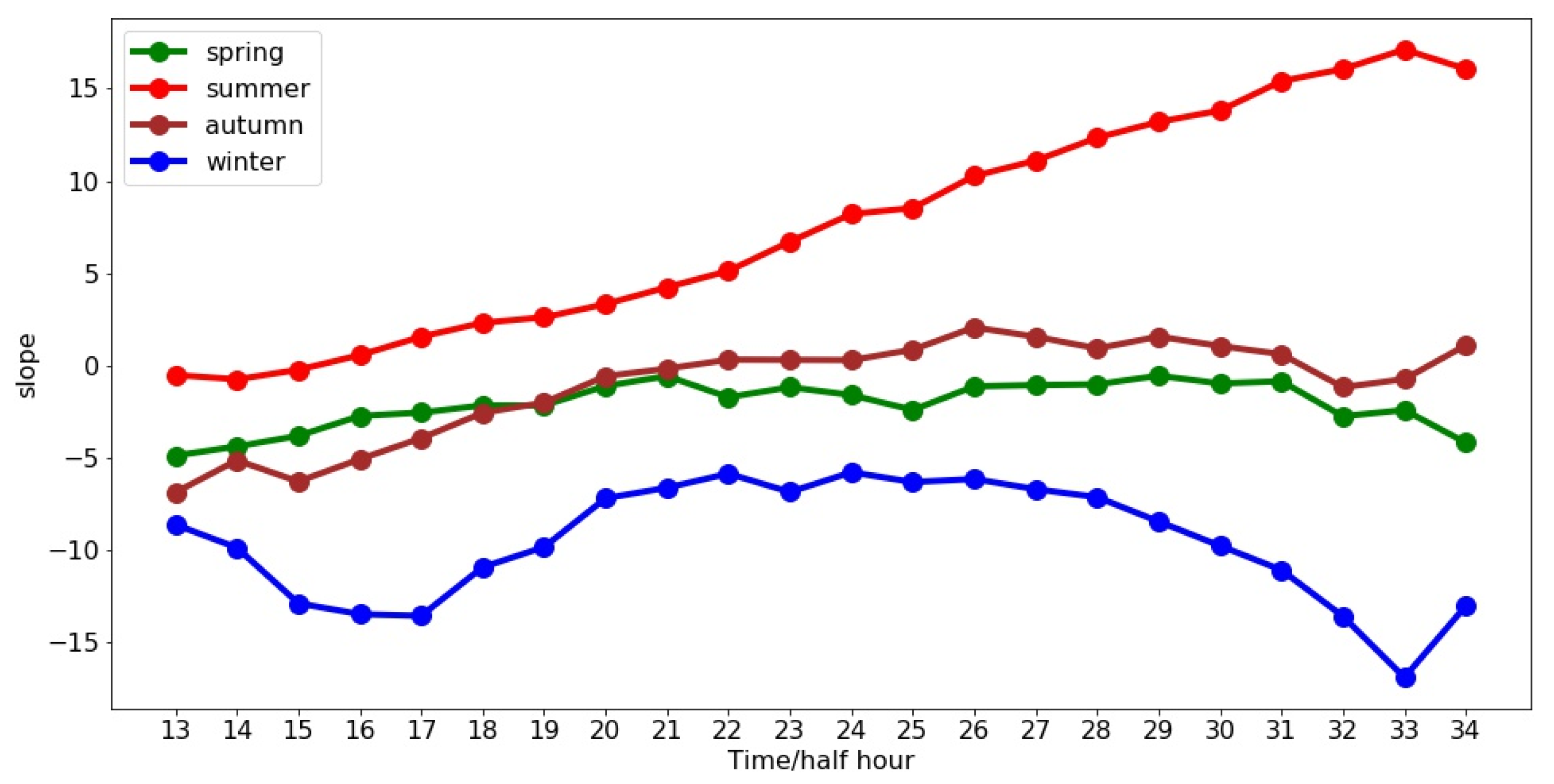
The Pearson correlation coefficient between average daily temperature and average daily load for each season are −0.48 (spring), 0.67 (summer), −0.36 (autumn), and −0.74 (winter). In other words, there is a strong correlation between temperature and actual consumption load. Therefore, we used absolute difference to find similar solar irradiation points in each season to match and offset the impact of PV output by making a difference to the net load of the corresponding day, and further used the least squares method to find the relationship between delta temperature and approximate actual load difference of each time stamp. Each solar irradiation point found the five most similar solar irradiation points to match. The slope of each time point of the linear fitting of temperature difference and load difference using the least squares method is shown in Figure 5. It can be observed that the slopes at different times in different seasons are inconsistent, and the positive and negative values of the slopes can also reflect the positive correlation between summer temperature and actual load, and the negative correlation among spring, autumn, and winter.

After obtaining the temperature-based sensitivity results of the actual load, the two-day load based on similar electricity consumption behavior can be corrected to the same temperature level according to the corresponding temperature difference (i.e., simulated as a situation where the electricity consumption behavior is as consistent as possible) during the analytic of the PV output power sensitivity.

When analyzing the sensitivity of PV output power, the $k$ value of k nearest neighbor was set to 15 to match load days with similar electricity consumption behavior. We used MLP to build a model of the relationship between delta solar irradiation and approximate delta PV output power. The MLP has a hidden layer with 20 hidden nodes, and the input-hidden layer and hidden-output layer are connected by the rectified linear unit (ReLU) and sigmoid function, respectively. The Adam optimizer was implemented in the MLP. In order to increase the training features of the sample, when building the MLP, in addition to delta solar irradiation, the solar irradiation of the two days before the difference was added as the input of the network.

Table 3. Accuracy comparison of PV output separation.

Season	Without Temperature Correction		With Temperature Correction
	MAE (kW)	RAE (%)	MAE (kW)	RAE (%)
Spring	56.47	62.21	27.79	30.61
Summer	70.25	78.42	30.76	34.34
Autumn	51.83	70.66	20.72	28.26
Winter	61.68	98.96	23.97	38.45

shows the comparison of the separation accuracy of the PV output curve before and after the correction. It can be observed from the table that after the temperature-based correction, the separation accuracy of the PV output power curve has been greatly improved. The value of RAE in spring, summer, autumn, and winter is decreased by 31.60%, 44.08%, 42.40%, and 60.51%, respectively.

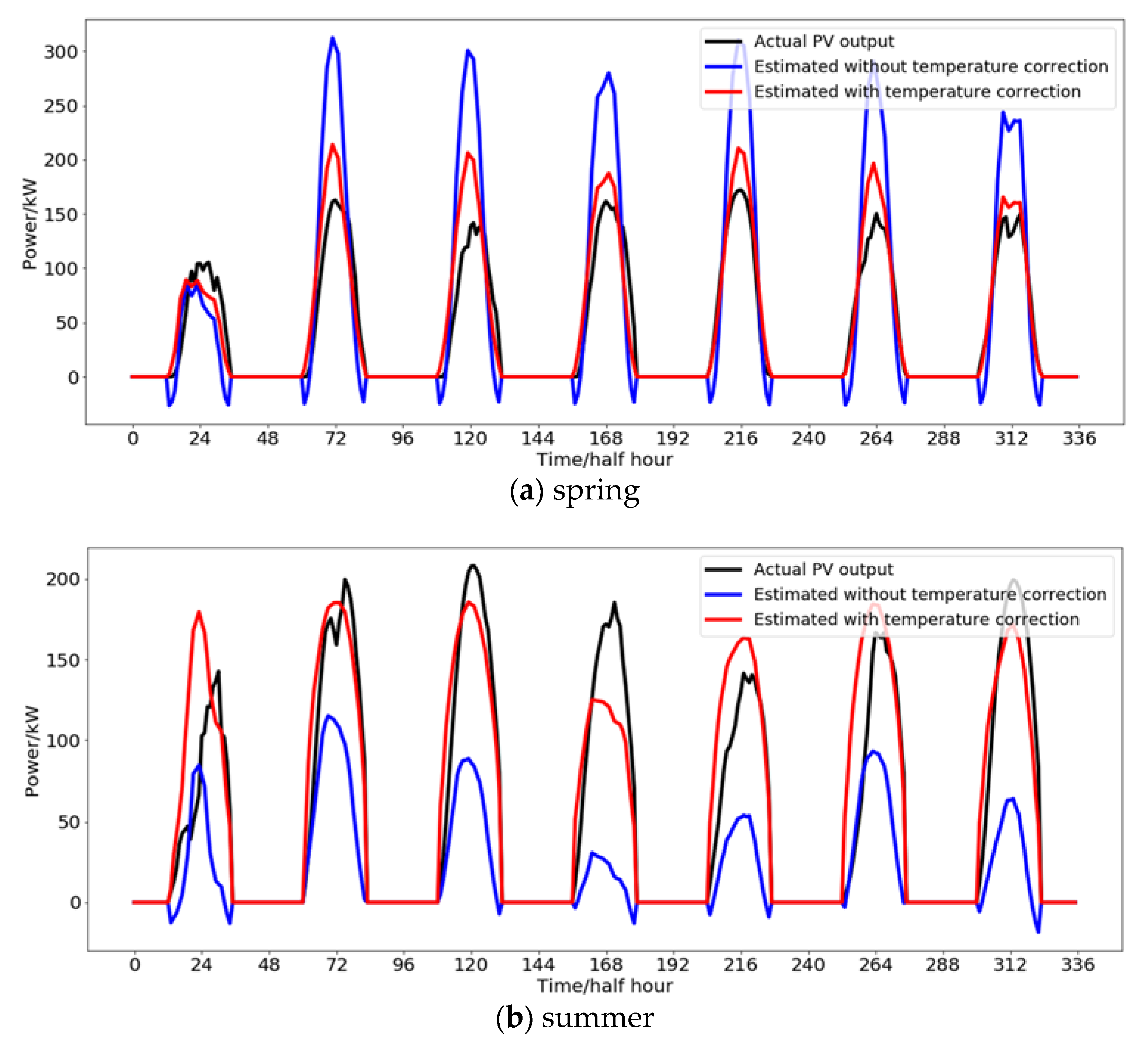
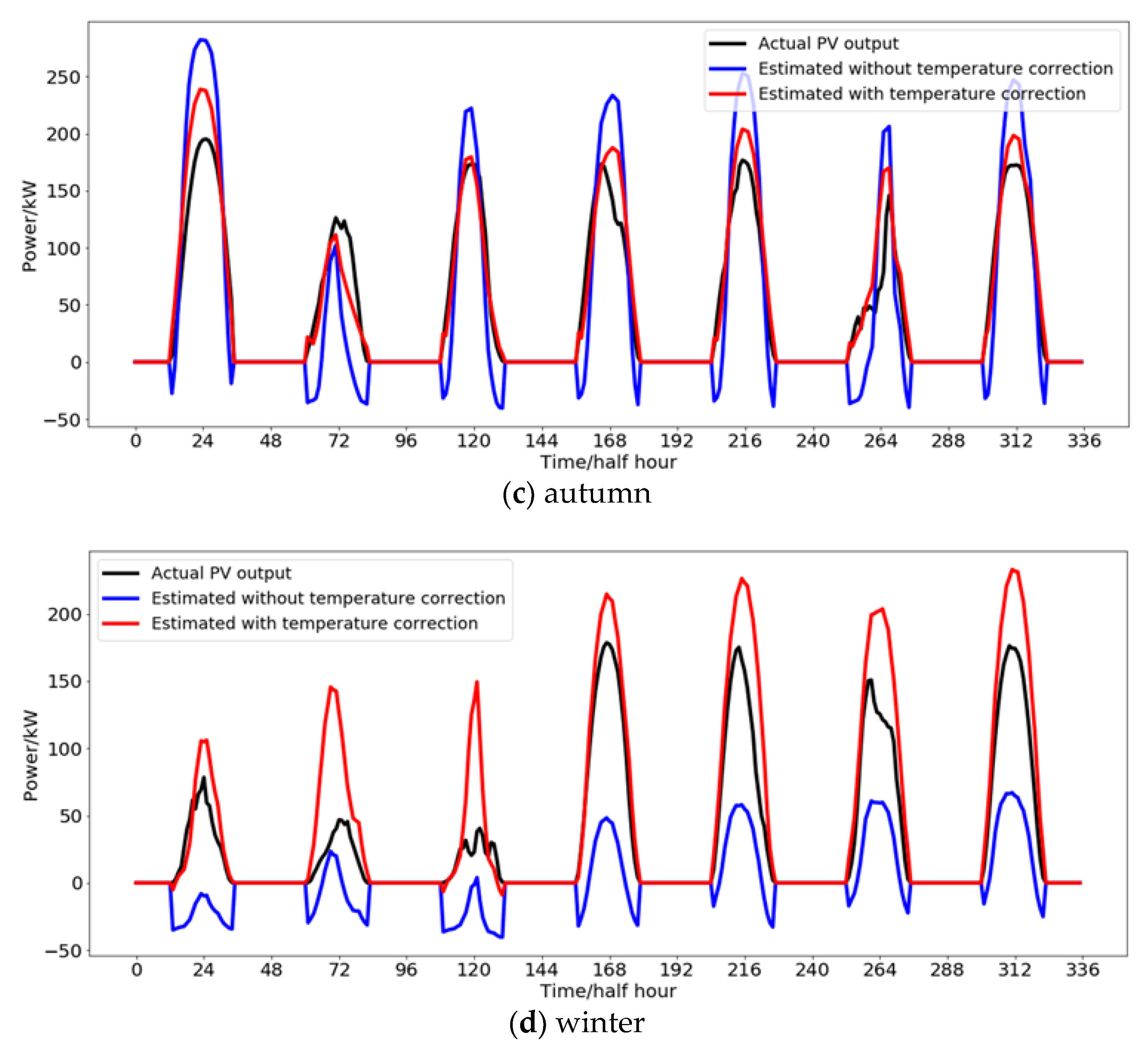
In order to more intuitively reflect the effectiveness of the proposed PV output decomposition method, Figure 6 shows the decomposition results of PV output power for a week in each season. It can be seen from the figure that without temperature-based correction, the estimated PV output power will appear negative, which is obviously not logical. The main reason for this problem is that, although we have used KNN to find dates with similar temperatures as much as possible to ensure that the electricity consumption behavior of users on the two days is consistent, however, in reality, it is almost impossible to find a pair of dates with exactly the same temperature change. Moreover, for periods of sunrise and sunset, the solar zenith angle is too small, which leads to very high sensitivity of PV output. When using neural networks to build PV output power estimation models, they are extremely susceptible to differences in electrical behavior caused by temperature differences. Therefore, the PV output power and solar irradiation will show a negative correlation. However, after the temperature-based correction, the negative value is eliminated, and there is also a certain improvement in the curve waveform.

4.3. Results and Analysis of CBL Prediction

Since none of the customers in the data set participated in the DR project, we chose the top 50 electricity consumption days in the data set as the DR days, because the DR event generally occurs when the electricity consumption is large, and the true value of CBL can be regarded as the historical net load value of the corresponding date. At the same time, we could not determine the specific time when the DR event occurred. We assumed the scenario of the DR event occurring at the moment when there was PV output power to reveal the effectiveness of the CBL prediction algorithm based on PV output separation.

The number of hidden layer units of MLP and RNN were set to 20, and the number of layers was set to 2. We performed 500 iterations for each network training. Historical load and temperature data of 30 days before DR days were used to train these two networks.

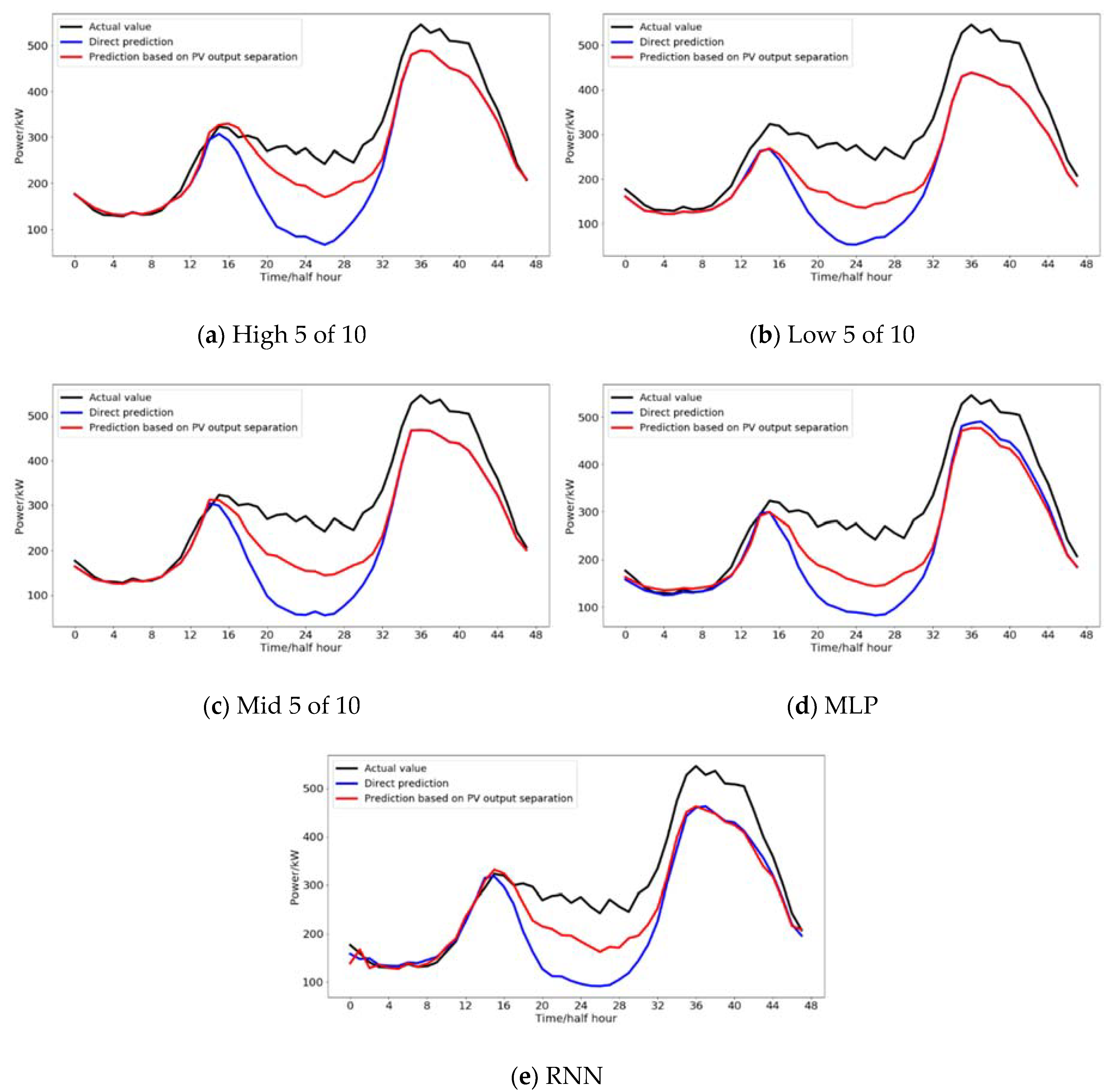
The comparison forecasting results of the five methods (High 5 of 10, Low 5 of 10, Mid 5 of 10, MLP, and RNN) of the CBL based on direct prediction and PV curve decomposition are shown in Figure 6, in which a certain DR event day is randomly selected as an example. In Figure 7, we can see that after using the proposed PV output power curve decomposition algorithm, the accuracy of all five CBL prediction methods has been improved.

Table 4. Average evaluation results of CBL prediction for overall days under different methods.

CBL Prediction Methods	Direct Prediction			Prediction Based on PV Output Separation
	MAE (kW)	Bias (kW)	RER	MAE (kW)	Bias (kW)	RER
High 5 of 10	73.46	−51.16	78.07	65.56	−45.44	79.34
Low 5 of 10	118.53	−115.00	79.28	102.05	−98.16	63.11
Mid 5 of 10	93.27	−82.33	77.19	80.36	−69.34	72.32
MLP	83.15	−74.76	76.44	74.49	−66.87	71.42
RNN	82.50	−71.69	72.42	69.15	−57.86	66.34

shows the average results of the evaluation indexes of CBL prediction for overall DR days under different methods.

From the MAE and RER in Table 4, it can be seen that after applying the PV output power curve decomposition algorithm, the errors of the three CBL prediction methods are reduced and the proposed method has a better stability. This is because through the PV output power curve decomposition, the PV output part can get relatively accurate forecasting results. Regardless of whether the PV output power curve is decomposed or not, the bias in the table is negative, indicating that the predicted CBL is generally smaller than the actual value. One of the explanations is that the selected DR days have a larger load. Therefore, these five CBL prediction methods provided in the calculation example can only obtain smaller values than the actual CBL. At the same time, we can also see that because High 5 of 10 uses the larger data in the first ten days for CBL prediction, this method has the highest accuracy.

5. Conclusions

This paper proposes a decomposition method of the behind-the-meter PV output power curve. The advantage of this method is that it can estimate the PV output power curve data of aggregated customers when only the historical net load data, historical temperature data, and historical PV data of aggregated customers are known, without the need for knowing individual distributed PV output system equipment information. The framework firstly searches for similar time points in historical solar irradiation data, makes a difference to the corresponding net load, and obtains the temperature-based sensitivity of actual load according to the least squares method. Then it finds the date with similar electricity consumption behavior to match and uses the temperature-based actual load sensitivity to correct the net load of the matched day to the same temperature standard and makes a difference to offset the actual load part. Finally, MLP is used to fit the relationship between the delta solar irradiation and delta approximate PV output power to derive the PV output power curve estimation model. To illustrate the effectiveness of the proposed PV output decomposition framework, a total of 300 real customers’ data sets containing PV output power from Ausgrid were used to simulate PV output decomposition experiments. At the same time, the results of the two types of prediction algorithms (average and regression) demonstrated that the CBL prediction based on PV output decomposition has better performance in MAE, bias, and RER.

In summary, this is a brand-new framework for BTM PV output estimation. Its most obvious characteristic advantage is that the algorithm does not depend on any data other than the historical net load data and weather data. In future work, the performance of the model will be analyzed more comprehensively, such as the impact of the resolution of the input data on the performance of the model, and the stability of the model under extreme weather conditions.

References

1. Wang, D.; Wu, R.; Li, X.; Lai, C.S.; Wu, X.; Wei, J.; Xu, Y.; Wu, W.; Lai, L.L. Two-stage optimal scheduling of air conditioning resources with high photovoltaic penetrations. J. Clean. Prod. 2019, 241, 118407. [Google Scholar] [CrossRef]
2. Lai, C.S.; McCulloch, M.D. Levelized cost of electricity for solar photovoltaic and electrical energy storage. Appl. Energy 2017, 190, 191–203. [Google Scholar] [CrossRef]
3. Zhao, Z.; Cheng, R.; Yan, B.; Zhang, J.; Zhang, Z.; Zhang, M.; Lai, L.L. A dynamic particles MPPT method for photovoltaic systems under partial shading conditions. Energy Convers. Manag. 2020, 220, 113070. [Google Scholar] [CrossRef]
4. Renewables 2020 Global Status Report–REN21. Available online: https://www.ren21.net/gsr-2020/chapters/chapter_01/chapter_01/ (accessed on 15 August 2020).
5. Lai, C.S.; Jia, Y.; Lai, L.L.; Xu, Z.; McCulloch, M.D.; Wong, K.P. A comprehensive review on large-scale photovoltaic system with applications of electrical energy storage. Renew. Sust. Energ. Rev. 2017, 78, 439–451. [Google Scholar] [CrossRef]
6. Hou, Q.; Du, E.; Zhang, N.; Kang, C. Impact of high renewable penetration on the power system operation mode: A data-driven approach. IEEE Trans. Power Syst. 2020, 35, 731–741. [Google Scholar] [CrossRef]
7. Xu, X.; Li, J.; Xu, Y.; Xu, Z.; Lai, C.S. A two-stage game-theoretic method for residential PV panels planning considering energy sharing mechanism. IEEE Trans. Power Syst. 2020, 35, 3562–3573. [Google Scholar] [CrossRef] [Green Version]
8. Xu, X.; Jia, Y.; Xu, Y.; Xu, Z.; Chai, S.; Lai, C.S. A multi-agent reinforcement learning based data-driven method for home energy management. IEEE Trans Smart Grid. 2020, 11, 3201–3211. [Google Scholar] [CrossRef] [Green Version]
9. Xu, X.; Li, J.; Xu, Z.; Zhao, J.; Lai, C.S. Enhancing photovoltaic hosting capacity-A stochastic approach to optimal planning of static var compensator devices in distribution networks. Appl. Energy 2019, 238, 952–962. [Google Scholar] [CrossRef] [Green Version]
10. Hippert, H.S.; Pedreira, C.E.; Souza, R.C. Neural networks for short-term load forecasting: A review and evaluation. IEEE Trans. Power Syst. 2001, 16, 44–55. [Google Scholar] [CrossRef]
11. Xu, F.Y.; Cun, X.; Yan, M.; Yuan, H.; Wang, Y.; Lai, L.L. Power market load forecasting on neural network with beneficial correlated regularization. IEEE Trans. Industr. Inform. 2018, 14, 5050–5059. [Google Scholar] [CrossRef]
12. Lai, C.S.; Mo, Z.; Wang, T.; Yuan, H.; Ng, W.W.Y.; Lai, L.L. Load forecasting based on deep neural network and historical data augmentation. IET Gener. Transm. Distrib. 2020. [Google Scholar] [CrossRef]
13. Lai, C.S.; Locatelli, G.; Pimm, A.; Tao, Y.; Li, X.; Lai, L.L. A financial model for lithium-ion storage in a photovoltaic and biogas energy system. Appl. Energy 2019, 251, 113179. [Google Scholar] [CrossRef]
14. Lai, C.S.; McCulloch, M.D. Sizing of stand-alone solar PV and storage system with anaerobic digestion biogas power plants. IEEE Trans. Ind. Electron. 2017, 64, 2112–2121. [Google Scholar] [CrossRef]
15. Wu, X.; Lai, C.S.; Bai, C.C.; Lai, L.L.; Zhang, Q.; Liu, B. Optimal kernel ELM and variational mode decomposition for probabilistic PV power prediction. Energies 2020, 13, 3592. [Google Scholar] [CrossRef]
16. Lai, C.S.; Jia, Y.; McCulloch, M.D.; Xu, Z. Daily clearness index profiles cluster analysis for photovoltaic system. IEEE Trans. Industr. Inform. 2017, 13, 2322–2332. [Google Scholar] [CrossRef]
17. Siano, P. Demand response and smart grids—A survey. Renew. Sust. Energ. Rev. 2014, 30, 461–478. [Google Scholar] [CrossRef]
18. Shariatzadeh, F.; Mandal, P.; Srivastava, A.K. Demand response for sustainable energy systems: A review, application and implementation strategy. Renew. Sust. Energ. Rev. 2015, 45, 343–350. [Google Scholar] [CrossRef]
19. Xu, F.Y.; Zhang, T.; Lai, L.L.; Zhou, H. Shifting boundary for price-based residential demand response and applications. Appl. Energy 2015, 146, 353–370. [Google Scholar] [CrossRef]
20. Xu, F.; Huang, B.; Cun, X.; Wang, F.; Yuan, H.; Lai, L.L.; Vaccaro, A. Classifier economics of Semi-Intrusive Load Monitoring. Int. J. Electr. Power Energy Syst. 2018, 103, 224–232. [Google Scholar] [CrossRef]
21. Wang, D.; Qiu, J.; Reedman, L.; Meng, K.; Lai, L.L. Two stage energy management for networked microgrids with high renewable penetrations. Appl. Energy 2018, 226, 39–48. [Google Scholar] [CrossRef]
22. Zheng, J.; Lai, C.S.; Yuan, H.; Dong, Z.Y.; Meng, K.; Lai, L.L. Electricity plan recommender system with electrical instruction-based recovery. Energy 2020, 203, 117775. [Google Scholar] [CrossRef]
23. Li, K.; Wang, F.; Mi, Z.; Fotuhi-Firuzabad, M.; Duić, N.; Wang, T. Capacity and output power estimation approach of individual behind-the-meter distributed photovoltaic system for demand response baseline estimation. Appl. Energy 2019, 253, 113595. [Google Scholar] [CrossRef]
24. Wang, F.; Li, K.; Wang, X.; Jiang, L.; Ren, J.; Mi, Z.; Shafie-khah, M.; Catalão, J.P.S. A distributed PV system capacity estimation approach based on support vector machine with customer net load curve features. Energies 2018, 11, 1750. [Google Scholar] [CrossRef] [Green Version]
25. Jazaeri, J.; Alpcan, T.; Gordon, R.; Brandao, M.; Hoban, T.; Seeling, C. Baseline methodologies for small scale residential demand response. In Proceedings of the 2016 IEEE Innovative Smart Grid Technologies Asia (ISGT-Asia), Melbourne, Australia, 28 November–1 December 2016. [Google Scholar]
26. Zhang, X.; Grijalva, S. A data-driven approach for detection and estimation of residential PV installations. IEEE Trans. Smart Grid. 2016, 7, 2477–2485. [Google Scholar] [CrossRef]
27. Shaker, H.; Manfre, D.; Zareipour, H. Forecasting the aggregated output of a large fleet of small behind-the-meter solar photovoltaic sites. Renew. Energy 2020, 147, 1861–1869. [Google Scholar] [CrossRef]
28. Landelius, T.; Andersson, S.; Abrahamsson, R. Modelling and forecasting PV production in the absence of behind-the-meter measurements. Prog. Photovolt. Res. Appl. 2019, 27, 990–998. [Google Scholar] [CrossRef] [Green Version]
29. Tazvinga, H.; Xia, X.; Zhang, J. Minimum cost solution of photovoltaic–diesel–battery hybrid power systems for remote consumers. Sol. Energy 2013, 96, 292–299. [Google Scholar] [CrossRef]
30. Wu, K.; Zhou, H. A multi-agent-based energy-coordination control system for grid-connected large-scale wind-photovoltaic energy storage power-generation units. Sol. Energy 2014, 107, 245–259. [Google Scholar] [CrossRef]
31. Kabir, F.; Yu, N.; Yao, W.; Yang, R.; Zhang, Y. Estimation of behind-the-meter solar generation by integrating physical with statistical models. In Proceedings of the 2019 IEEE International Conference on Communications, Control, and Computing Technologies for Smart Grids (SmartGridComm), Beijing, China, 21–23 October 2019. [Google Scholar]
32. Shaker, H.; Zareipour, H.; Wood, D. A data-driven approach for estimating the power generation of invisible solar sites. IEEE Trans. Smart Grid. 2016, 7, 2466–2476. [Google Scholar] [CrossRef]
33. Cheung, C.M.; Zhong, W.; Xiong, C.; Srivastava, A.; Kannan, R.; Prasanna, V.K. Behind-the-meter solar generation disaggregation using consumer mixture models. In Proceedings of the 2018 IEEE International Conference on Communications, Control, and Computing Technologies for Smart Grids (SmartGridComm), Aalborg, Denmark, 29–31 October 2018. [Google Scholar]
34. Cheung, C.M.; Kuppannagari, S.R.; Kannan, R.; Prasanna, V.K. Disaggregation of behind-the-meter solar generation in presence of energy storage resources. In Proceedings of the 2020 IEEE Conference on Technologies for Sustainability (SusTech), Santa Ana, CA, USA, 23–25 April 2020. [Google Scholar]
35. Qiu, Y.; Kahn, M.E.; Xing, B. Quantifying the rebound effects of residential solar panel adoption. J. Environ. Econ. Manag. 2019, 96, 310–341. [Google Scholar] [CrossRef]
36. Pouraltafi-kheljan, S.; Göl, M. Power generation nowcasting of the behind-the-meter photovoltaic systems. arXiv 2020, arXiv:2001.02157. [Google Scholar]
37. Chen, Y.; Xu, P.; Chu, Y.; Li, W.; Wu, Y.; Ni, L.; Bao, Y.; Wang, K. Short-term electrical load forecasting using the Support Vector Regression (SVR) model to calculate the demand response baseline for office buildings. Appl. Energy 2017, 195, 659–670. [Google Scholar] [CrossRef]
38. Wijaya, T.K.; Vasirani, M.; Aberer, K. When bias matters: An economic assessment of demand response baselines for residential customers. IEEE Trans. Smart Grid. 2014, 5, 1755–1763. [Google Scholar] [CrossRef]
39. Wang, F.; Li, K.; Liu, C.; Mi, Z.; Shafie-Khah, M.; Catalão, J.P.S. Synchronous pattern matching principle-based residential demand response baseline estimation: Mechanism analysis and approach description. IEEE Trans. Smart Grid. 2018, 9, 6972–6985. [Google Scholar] [CrossRef]
40. Park, S.; Ryu, S.; Choi, Y.; Kim, J.; Kim, H. Data-driven baseline estimation of residential buildings for demand response. Energies 2015, 8, 10239–10259. [Google Scholar] [CrossRef] [Green Version]
41. Haas, R.; Auer, H.; Biermayr, P. The impact of consumer behavior on residential energy demand for space heating. Energy Build. 1998, 27, 195–205. [Google Scholar] [CrossRef]
42. Hatton, L.; Charpentier, P.; Matzner-Lober, E. Statistical estimation of the residential baseline. IEEE Trans. Power Syst. 2016, 31, 1752–1759. [Google Scholar] [CrossRef]
43. Wu, X.; Wu, R.; Wang, D.; Wei, J.; Li, X.; Lai, L.L.; Lai, C.S. Coordinated air conditioning resources scheduling with high photovoltaic penetrations. In Proceedings of the 2018 International Conference on Power System Technology (POWERCON), Guangzhou, China, 6–8 November 2018. [Google Scholar]
44. Mu, Y.; Liu, X.; Wang, L. A Pearson’s correlation coefficient based decision tree and its parallel implementation. Inf. Sci. 2018, 435, 40–58. [Google Scholar] [CrossRef]
45. Pinson, P.; Nielsen, H.A.; Madsen, H.; Nielsen, T.S. Local linear regression with adaptive orthogonal fitting for the wind power application. Stat. Comput. 2008, 18, 59–71. [Google Scholar] [CrossRef] [Green Version]
46. Keller, J.M.; Gray, M.R.; Givens, J.A. A fuzzy k-nearest neighbor algorithm. IEEE Trans. Syst. Man Cybern. Syst. 1985, 15, 580–585. [Google Scholar] [CrossRef]
47. Taud, H.; Mas, J.F. Multilayer Perceptron (MLP). In Geomatic Approaches for Modelling Land Change Scenarios; Springer: Berlin, Germany, 2018; pp. 451–455. [Google Scholar]
48. Kim, J.; Moon, J.; Hwang, E.; Kang, P. Recurrent inception convolution neural network for multi short-term load forecasting. Energy Build. 2019, 194, 328–341. [Google Scholar] [CrossRef]
49. Renewables.ninjia. Available online: https://www.renewables.ninja/ (accessed on 15 August 2020).
Figure 1. Example of the composition of net load.
Forecasting 02 00025 g001
Figure 2. An example of the relationship between delta temperature and delta actual load at 17:00 in winter and summer.
Forecasting 02 00025 g002
Figure 3. Flowchart of photovoltaic (PV) output power decomposition.
Forecasting 02 00025 g003
Figure 4. Clusters of actual load curves of (a) spring, (b) summer, (c) autumn and (d) winter.
Forecasting 02 00025 g004
Figure 5. Slope of the linear fitting of delta temperature and approximate delta actual load.
Forecasting 02 00025 g005
Figure 6. Estimated PV output power curves for a week.
Forecasting 02 00025 g006aForecasting 02 00025 g006b
Figure 7. Comparison of direct prediction and customer baseline (CBL) prediction results based on PV output curve decomposition on a certain demand response (DR) day.
Forecasting 02 00025 g007