Abstract
Reference intervals play an important role in medicine, for instance, for the interpretation of blood test results. They are defined as the central 95% values of a healthy population and are often stratified by sex and age. In recent years, so-called indirect methods for the computation and validation of reference intervals have gained importance. Indirect methods use all values from a laboratory, including the pathological cases, and try to identify the healthy sub-population in the mixture of values. This is only possible under certain model assumptions, i.e., that the majority of the values represent non-pathological values and that the non-pathological values follow a normal distribution after a suitable transformation, commonly a Box–Cox transformation, rendering the parameter of the Box–Cox transformation as a nuisance parameter for the estimation of the reference interval. Although indirect methods put high effort on the estimation of , they come to very different estimates for , even though the estimated reference intervals are quite coherent. Our theoretical considerations and Monte-Carlo simulations show that overestimating can lead to intolerable deviations of the reference interval estimates, whereas produces usually acceptable estimates. For close to 1, its estimate has limited influence on the estimate for the reference interval, and with reasonable sample sizes, the uncertainty for the -estimate remains quite high.
1. Introduction
Reference intervals are among the most important interpretation aids in laboratory medicine. By definition, they comprise the central 95 percent of a presumably healthy reference population [1] and thus indicate the probability of whether an observed laboratory result is to be classified as “normal” or “pathological”.
In the so-called direct methods for determining a reference interval, one performs a sufficient number of measurements on a presumably healthy reference collective and determines the quantiles 0.025 and 0.975 either non-parametrically or parametrically under the assumption of a certain distribution (e.g., Gaussian). More significant in medical practice are indirect estimation methods based on routinely collected laboratory results from laboratory information systems [2]. Since these always represent mixtures of normal and pathological values, the estimation of the respective quantiles is only possible under the assumption of an underlying distribution model for the sub-collective of the healthy reference population contained therein.
For practical reasons, some authors rely on only one or two different distribution models, e.g., lognormal distribution for all kinds of quantitative results [3] or a choice between Gaussian for symmetrically distributed and lognormal for right-skewed data [4]. However, in the recent literature there is a trend to assume a continuum of distributions of different skewnesses, which can be represented by a normal distribution after the Box–Cox transformation of the original data using a lambda exponent between 0 and 1 or slightly beyond these limits [5,6,7,8,9].
The motivation to perform this study results from the observation that the application of different published algorithms to identical laboratory data [10] provides a very weak correlation between estimates (see Figure 1). Hence, the question arises whether state-of-the-art procedures are suitable at all to optimise values under the specific conditions of indirect reference interval estimation. Our results seem to indicate that the reliability of estimates is poor even in ideal theoretical distributions and close to pure guesswork in mixed populations including pathological values as one would find them in real data sets from laboratory information systems.
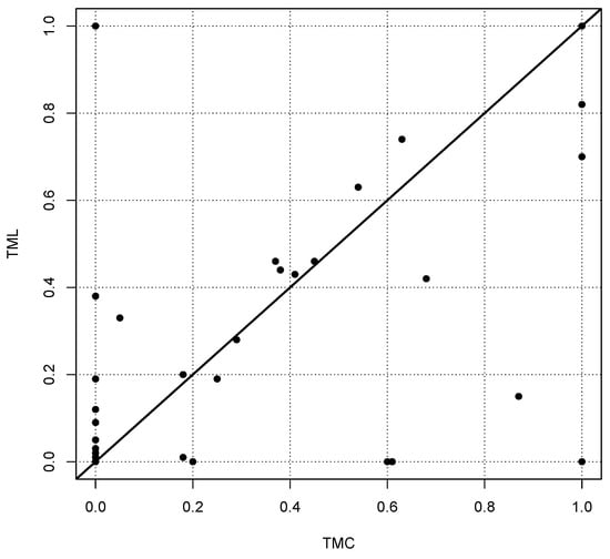
Figure 1.
Estimates of the parameter for the Box–Cox transformation for 66 reference intervals for two different algorithms, called TMC (Truncated Minimum Chi-square, see [8]) and TML (Truncated Maximum Likelihood, see [5]). Each point represents the two values estimated by TMC and TML. In the ideal case, the estimates should be on the diagonal shown as a bold line. The estimated values have been taken from the supplementary Table 3, published in [10]. It should be noted that more than one-third of the values are concentrated at the origin of the coordinate system, i.e., for the methods show a certain coherence.
The Pearson, Spearman and Kendall correlations between the two methods compared in Figure 1 are 0.60, 0.51 and 0.46, respectively. Comparing other methods yields similar poor correlations, although the estimated reference intervals are in most cases very similar. A similar result was observed by Meyer et al. (see Figure 6 in [11]).
The aim of this paper is not to provide a new indirect method for the estimation of reference intervals but to investigate whether it is meaningful to incorporate an arbitrary Box–Cox transformation involving the estimation of its parameter . We do not question the assumption that the values from the healthy sub-population originate from a Box–Cox transformed (truncated) normal distribution. This assumption is common to all state-of-the-art indirect methods for the estimation of reference intervals. It might be advantageous to replace the (truncated) normal distribution by another family of distributions, e.g., the Weibull distribution, yielding only positive values, or to replace the Box–Cox transformation with a Yeo–Johnson transformation [12] that can also handle negative values. We leave such ideas to further research in the future. Our main aim is to demonstrate that the standard indirect methods for reference interval estimation pay a high price in terms of computational costs to estimate the parameter of an arbitrary Box–Cox transformation without a significant benefit. The estimation of alone does not lead to high computational effort. But the combination of sorting out the pathological values and finding the optimal value for simultaneously requires iterative methods and high computational costs.
In the following, we analyse the influence and uncertainty of the nuisance parameter in the context of reference interval estimation based on theoretical considerations and simulations. We deliberately restrict our investigations to the ideal context without pathological values. If the estimation of incorporates high uncertainty and the influence of a wrong estimation of is also quite limited in this ideal setting, then it is obvious that estimating in the more complex situation including pathological values is an academic task with little improvement for the results.
Section 2 provides a formal definition of the statistical problem that we consider here. Section 3 investigates the effect of a wrong estimate for on the reference interval estimate for infinite sample sizes-based Monte-Carlo simulations. Finite sample sizes are considered to quantify the uncertainty involved in the estimation of in Section 4. In the final discussion, we review our results and conclude that an exact estimation of the nuisance parameter is of limited benefit for reference intervals because it is afflicted with a high uncertainty, whereas a wrong estimation does not have a strong influence on the estimate for the reference interval.
2. Problem Formulation
Indirect methods for the estimation of reference intervals in laboratory medicine aim to estimate the 2.5% and the 97.5% quantiles of the healthy sub-population. It is not known which of the values belong to the healthy sub-population. Formally speaking, we have a sample of non-negative values from a mixture of distributions and we want to estimate the 2.5% and the 97.5% quantiles of one specific distribution in this mixture. It is obvious that—without further assumptions—this is an ill-defined task. Therefore, it is usually assumed that the specific distribution of interest represents the majority of values and follows (approximately) a normal distribution after a Box–Cox transformation. The challenge is then to estimate the parameter and simultaneously the expected value and the standard deviation of the normal distribution, which corresponds to the subset of values from the healthy population after the Box–Cox transformation. We argue that a reliable estimation of is more or less impossible in a realistic setting. In order to show this, we even assume that there are no pathological values, i.e., all values originate from the healthy population.
In mathematical terms, the problem is defined as follows. A sample is generated from a normal distribution truncated at 0, representing the healthy population after the Box–Cox transformation
with parameter . The truncation at 0 is necessary because the Box–Cox transformation can only be applied to positive values. It is assumed that the truncation is more or less negligible, i.e., the parameters and of the normal distribution lead to a very small probability for negative values for the normal distribution. In any case, the 2.5% quantile must be above 0. In principle, one could use the Yeo–Johnson transformation [12]. But this does not seem to be a common practice in laboratory medicine.
Let , i.e., X is a random variable following a normal distribution with expected value and variance , which is left-truncated at 0. We observe the random variable where is the inverse Box–Cox transformation
The parameters , and are not known. Our aim is to estimate the 2.5% and the 97.5% quantiles of .
It should be emphasised again that we consider the ideal case where we observe only values from the healthy population without any pathological values, so that we do not consider the more complex case of a mixture of distributions in which the healthy sub-population is only one part of the mixture model.
The aim of this paper is to show the following in a realistic setting:
- The estimation of will involve very high uncertainty;
- But this uncertainty has limited influence on the estimation of the 2.5% and the 97.5% quantiles.
3. Theoretical Analysis of Wrong Estimation of the Nuisance Parameter
We first analyse the influence of a wrong estimation of the parameter on the estimations of the 2.5% and the 97.5% quantiles. We assume that we observe the random variable where and we have a possibly wrong estimate for the parameter . From this estimate, we assume that the “true” underlying truncated normal distribution is for which we use estimates of the expected value and the standard deviation to estimate its 2.5% and 97.5% quantiles. These quantiles are then transformed by the inverse Box–Cox transformation to obtain estimates for the limits of the reference intervals. Figure 2 illustrates the situation we consider.
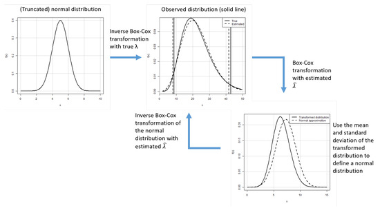
Figure 2.
Scenario for the analysis of the influence of the wrong estimation of the parameter for infinite sample sizes.
In this section, it is assumed that the estimations for and are based on a (infinite) sample from the distribution where . Because the corresponding integrals have no obvious solutions, we use a sample size of n = 100,000 to estimate and by the corresponding mean and sample standard deviation of the sample, i.e., we generated 100,000 values from a truncated normal distribution with expected value and standard deviation and applied the transformation to obtain the theoretical “wrong” estimates and .
We vary the true value for between 0 and 1. Without a loss of generality, we assume that the lower limit of the reference interval is at 1. This can always be achieved by changing or scaling the measurement units. The upper limit of the reference interval is varied between slightly above 1 and up to 50. In order to quantify the error of the estimated reference interval caused by the wrong estimate for , we measure the difference in terms of the zlog value that was introduced in [13]. The zlog value is a transformation based on a logarithmic transformation and a normalisation such that logarithms of the reference interval limits are mapped to the 2.5% and the 97.5% quantiles of a standard normal distribution. Thus, the reference interval is transformed to the range []:
where is the cumulative distribution function of the standard normal distribution.
Figure 3 shows the absolute zlog deviation for the lower (a) and upper (b) limit of the reference interval depending on and the upper limit of the reference interval when the lower limit is fixed at 1.
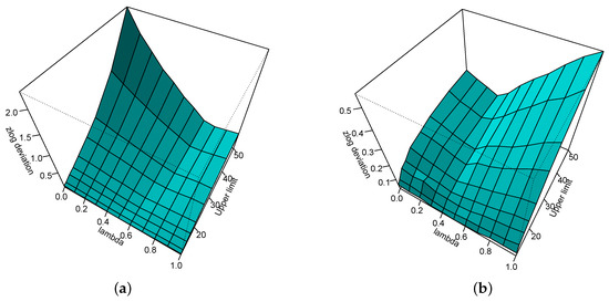
Figure 3.
Absolute zlog deviation for the lower (a) and upper (b) limit of the reference interval depending on and the upper limit of the reference interval when the lower limit is fixed at 1.
It can be seen that the effect of the wrong estimation to the estimate of the upper limit of the reference interval is quite limited, never exceeding the value of 0.5. The effect on the lower limit of the reference interval is high for values close to zero and a large upper limit of the reference interval.
Figure 4 zooms into Figure 3, showing the results only for a maximum upper limit of the reference interval of 30. It can be seen that for , a wrong estimate of has very little influence on the estimate of the upper limit of the reference interval and only when there is a non-negligible effect on the estimate for the lower limit of the reference interval.
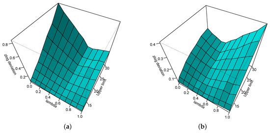
Figure 4.
Absolute zlog deviation for the lower (a) and upper (b) limit of the reference interval depending on and the upper limit of the reference interval—here bounded to 30—when the lower limit is fixed at 1.
In order to further analyse the influence of a wrong estimate for on the estimate of the reference interval, we consider the observed distribution where . Figure 5a shows the estimate of the upper limit for and wrong estimate between 0 and 1. The dotted line is the true upper limit of the reference interval. The curve indicates the estimated upper limit of the reference interval depending on . Figure 5b shows the same for .
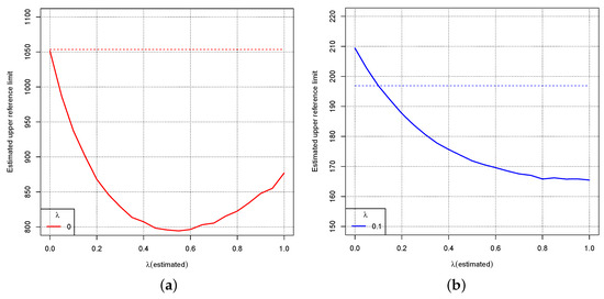
Figure 5.
Dotted lines: True upper limit of the reference interval for the distribution where for (a) and (b). The curves show the estimated upper limit of the reference interval depending on the wrong estimate for .
Figure 6b shows the same as Figure 5 for . Figure 6a shows the same for the lower limit of the reference interval including the values 0 and 0.1 for .
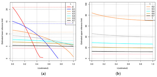
Figure 6.
Dotted lines: True lower (a) and upper (b) limit of the reference interval for the distribution where for different values of . The curves show the estimated lower (a) and upper (b) limit of the reference interval depending on the wrong estimate for .
Figure 5 and Figure 6 indicate again that a wrong estimate for the parameter will not affect the estimate for the reference interval drastically unless is close to 0, i.e., the Box–Cox transformation should be close to the logarithmic transformation. For close to 1, even a completely wrong estimate shows little effect on the estimates for the reference intervals. For smaller values of , an overestimation of implies high errors for the reference interval estimate. Figure 5 and Figure 6 might even suggest that always choosing leads to small errors with respect to the reference interval.
The observation is supported by investigating critical values of more closely where the logarithmic transformation could lead to unacceptable results for the reference interval. In [14], an equivalence test was proposed to check whether the deviation of an estimated reference interval from a given reference interval can be considered to be relevant in medical terms.
Figure 7 zooms into Figure 6 for and shows the ranges for which the equivalence test according to [14] would not reject the corresponding estimated reference limits as black lines. For both limits of the reference interval, the logarithmic transformation yields acceptable deviations in terms of the equivalence test, although the upper reference limit is almost at the boundary of the acceptance range. However, if is overestimated, i.e., for , the lower limit of the reference interval can no longer be accepted.
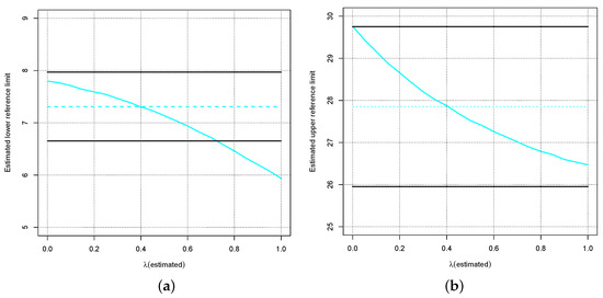
Figure 7.
Blue dotted lines: True lower (a) and upper (b) limit of the reference interval for the distribution where . The curves show the estimated lower (a) and upper (b) limit of the reference interval depending on the wrong estimate for . The black lines indicate the ranges for which the tolerance test according to [14] would not reject the corresponding estimated reference limits.
Not shown here are the similar results that yields.
4. Influence of the Sample Size
After having shown in the previous section that a correct estimation of is only important for the estimate of the reference interval when is close to 0, this section investigates the uncertainty of the estimate depending on the sample size.
We use the same observed distribution as in the previous section, i.e., where for . The sample sizes are varied between 100 and 1000. For each value and each sample size, we executed 10,000 Monte-Carlo simulations to obtain estimates for and the reference interval. For estimating , three methods were used: the probability plot correlation coefficient (PPCC), the Shapiro–Wilk test and a maximum likelihood estimator (log-likelihood). Based on the estimated , the data are Box–Cox transformed, the mean and standard deviation of the transformed data are computed and the 2.5% and the 97.5% quantiles of the normal distribution are determined. The estimates for the reference interval are obtained by applying the corresponding inverse Box–Cox transformation to the quantiles. In addition, the reference interval is also estimated directly based on the sample’s corresponding quantiles.
Figure 8 shows the results for for the lower (a) and upper (b) limit of the reference interval. The sample size is indicated on the x-axis, and the values for the limit of the reference interval are on the y-axis. The grey line indicates the true limit of the reference interval. The coloured curves show the 95% confidence interval for the estimate of the limit of the reference interval based on 10,000 Monte-Carlo simulations for the above-mentioned estimation methods. The black curve represents the 95% confidence interval when the limit of the reference interval is estimated directly by the corresponding sample quantile. The three different methods for estimation—the coloured lines—lead to almost exactly the same confidence intervals for the reference interval. The confidence intervals based on the sample quantiles are broader, which is no surprise because they do not make use of the fact that the data originate from a normal distribution to which an inverse Box–Cox transformation was applied.
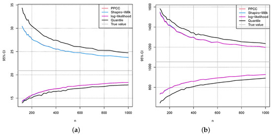
Figure 8.
For each sample size, 10,000 samples from the distribution where were taken to compute the 95% Monte-Carlo confidence intervals for the lower (a) and upper (b) limit of the reference interval depending on the sample size. The grey line indicates the true limit of the reference interval. The coloured lines use estimations for the reference intervals based on an estimate of . The black line is the 95% confidence interval when the 2.5% and the 97.5% sample quantiles are directly used for the reference interval.
Figure 9 and Figure 10 show the same results as in Figure 8 for the values and , respectively. Comparing the confidence intervals in Figure 8, Figure 9 and Figure 10 to the errors caused by a wrong estimation of in Figure 5 and Figure 6, one can see that they are in a similar range.
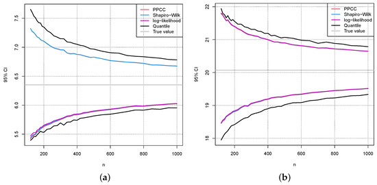
Figure 9.
The same as in Figure 8 (a) and (b), except that is chosen.
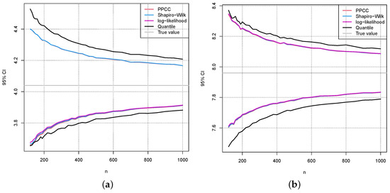
Figure 10.
The same as in Figure 8 (a) and (b), except that is chosen.
Figure 11 shows the 95% confidence intervals for the parameter depending on the sample size. For , the confidence intervals cover almost the full interval for the small samples sizes and make it impossible to obtain a reliable estimate for in these cases. The maximum likelihood method was used here for estimating . But the other mentioned methods yield very similar results.
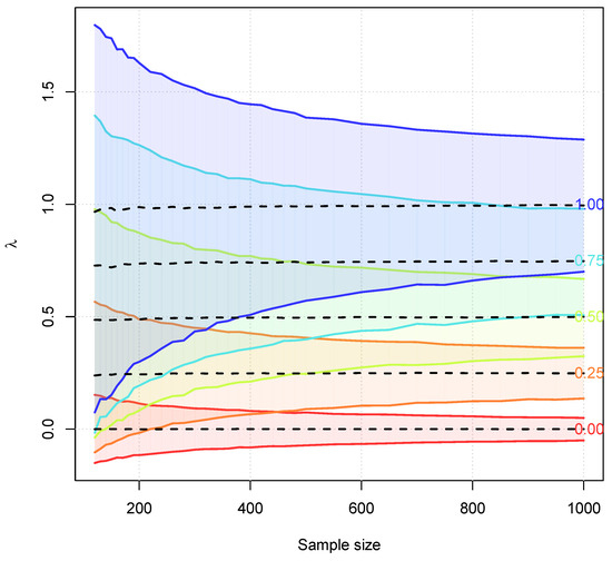
Figure 11.
Dotted lines correspond to the mean of the estimates for based on 10,000 Monte-Carlo simulations. The shaded areas and the lines are based on the 95% confidence intervals for .
Finally, we also apply one of the established indirect methods for reference interval estimation to the ideal simulated data to demonstrate that the estimation of is a daunting task when is close to 1. For each of the sample sizes , we have carried out 100 simulations, i.e., generated data 100 times from a truncated normal distribution with a Box–Cox transformation with . Figure 12 shows the box plots for the 100 estimates for each of the simulated sample sizes. The estimates were computed using the indirect method RefineR [9].
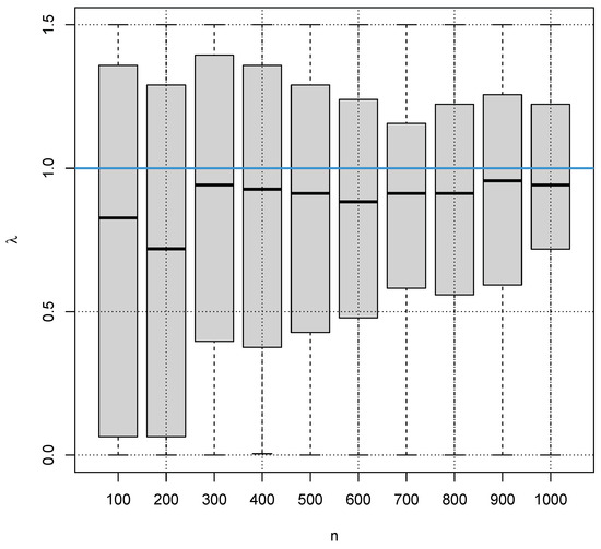
Figure 12.
Box plots for the estimates of the indirect method RefineR for 100 simulations for different samples n from the distribution with a Box–Cox transformation with (blue line).
It is obvious that the methods are close to random guessing for estimation in the case of smaller sample sizes, and even for larger sample sizes, the estimates for carry a high uncertainty. It also obvious that the methods seems to have a bias, systematically underestimating . Although this is not a desirable property in terms of statistics, it seems to be beneficial for the estimation of the reference intervals because we have seen that overestimating can lead to quite wrong reference interval estimates, whereas underestimating still produces reasonable reference interval estimates.
Figure 13a,b show the corresponding box plots for the estimates of the lower and upper limit of the reference interval, respectively. The method seems to have a bias tending to too narrow reference intervals. The bias decreases with increasing sample size.
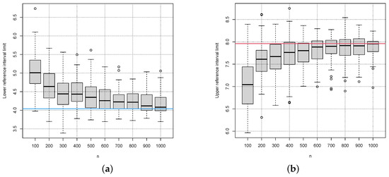
Figure 13.
Box plots for the estimates of lower (a) and upper (b) reference interval limit of the indirect method RefineR for 100 simulations for different samples n from the distribution with a Box–Cox transformation with . The red and blue lines indicate the true lower (blue line) and true upper limit (red line) of the reference interval.
Figure 10 shows much better results than RefineR in Figure 13. This is, however, an unfair comparison because RefineR was designed to deal with mixed populations including pathological values, whereas the methods in Figure 10 only work under the ideal assumption of an exclusively healthy population.
It is notable that a wrong estimate for does not show a high correlation with wrong estimates for the reference limits as Figure 14 indicates, where the absolute errors for the estimates are shown on the x-axis and the absolute errors for the estimates of the reference interval limits are shown on the y-axes.
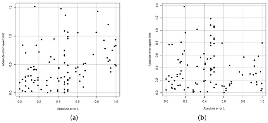
Figure 14.
RefineR’s absolute errors of the estimate and the lower (a) and upper (b) reference interval limit for sample size .
Other indirect methods yield similar results as RefineR for the simulated ideal data. The results are therefore not shown here.
5. Discussion and Conclusions
The advantage of indirect methods for reference interval estimation and verification is that they do not require a careful selection and examination of a healthy sub-population and they avoid ethical considerations, i.e., they rely on measurements of blood samples that were needed and taken for other reasons [2]. This is especially important when reference intervals for young children are considered where ethical reasons make it difficult to collect larger amounts of blood samples just for reference interval validation. The price that needs to be paid is that additional distributional assumptions cannot be avoided in order to at least roughly identify the healthy sub-population among a mixed sample from healthy and pathological cases. The usual assumptions are that the healthy sub-population contributes the majority of values and follows a normal distribution after a “suitable” transformation. The overlap of the healthy sub-population with “pathological distributions” should also be limited [15]. It is generally agreed that some kind of Box–Cox transformation should be applied to the data. The crucial question that was discussed in this paper is whether the full range of the parameter for the Box–Cox transformation should be considered or whether it might be sufficient to restrict the choice between and , meaning that the values of the healthy sub-population follow a lognormal or a normal distribution. The advantage of this restriction would also be the avoidance of the otherwise required truncation for arbitrary Box–Cox transformations.
In order to keep our analysis simple, we have restricted our investigations to the idealised case where we only deal with the healthy sub-population. If arbitrary Box–Cox transformations turn out to be of limited benefit even in this ideal case, the advantage of arbitrary Box–Cox transformation in the much more complicated setting of mixed populations might be questionable. Similar weak correlations between values estimated with different methods on identical data sets have also been observed by [11]. More general transformations, e.g., Box–Cox transformations with an additional shift parameter as mentioned in [10], make the situation even more difficult and lead to less interpretable results.
Our analyses have shown that a wrong estimate for has very limited influence on the resulting estimate for the reference interval when is greater than 0.6. For smaller values, it is important to not overestimate . Otherwise, the upper reference limit will be too low. An underestimation of by leads to tolerable errors for the reference interval in terms of an equivalence test described in [14].
Another result of our analyses is that at least for sample sizes clearly below 1000, the uncertainty for the estimation of remains relatively high so that a reliable estimate cannot be expected. A minimal sample size of 1000 has also been mentioned in [16].
Taking these results together, it might be sufficient to just consider the two options and . This would also lead to a significant speed-up of the often very slow algorithms for indirect reference interval estimation because these algorithm try to estimate , the healthy sub-population and its parameters at the same time, involving long iterative procedures.
Author Contributions
Conceptualisation, F.K. and G.H.; methodology, F.K. and G.H.; software, F.K. and N.R.; validation, G.H. and N.R.; formal analysis, F.K.; investigation, G.H., F.K. and N.R.; resources, F.K.; writing—original draft preparation, F.K.; writing—review and editing, G.H. and N.R.; visualisation, F.K. and N.R.; supervision, F.K. and G.H.; project administration, F.K. All authors have read and agreed to the published version of the manuscript.
Funding
This research received no external funding.
Institutional Review Board Statement
Not applicable.
Informed Consent Statement
Not applicable.
Data Availability Statement
No new data were created or analyzed in this study. Data sharing is not applicable to this article.
Conflicts of Interest
Author Georg Hoffmann was employed by the company Medizinischer Fachverlag Trillium GmbH. The remaining authors declare that the research was conducted in the absence of any commercial or financial relationships that could be construed as a potential conflict of interest.
References
- Horowitz, G.; Altaie, S.; Boyd, J.C.; Ceriotti, F.; Garg, U.; Horn, P.; Pesce, A.; Sine, H.E.; Zakowski, J. Defining, Establishing, and Verifying Reference Intervals in the Clinical Laboratory; Tech Rep Document EP28-A3C; Clinical & Laboratory Standards Institute: Wayne, PA, USA, 2010. [Google Scholar]
- Jones, G.; Haeckel, R.; Loh, T.; Sikaris, K.; Streichert, T.; Katayev, A.; Barth, J.; Ozarda, Y. Indirect methods for reference interval determination: Review and recommendations. Clin. Chem. Lab. Med. 2019, 57, 20–29. [Google Scholar] [CrossRef] [PubMed]
- Haeckel, R.; Wosniok, W. Observed, unknown distributions of clinical chemical quantities should be considered to be log-normal: A proposal. Clin. Chem. Lab. Med. 2010, 48, 1393–1396. [Google Scholar] [CrossRef] [PubMed]
- Klawonn, F.; Hoffmann, G.; Orth, M. Quantitative laboratory results: Normal or lognormal distribution. J. Lab. Med. 2020, 44, 143–150. [Google Scholar] [CrossRef]
- Arzideh, F.; Wosniok, W.; Gurr, E.; Hinsch, W.; Schumann, G.; Weinstock, N.; Haeckel, R. A plea for intra-laboratory reference limits. Part 2. A bimodal retrospective concept for determining reference limits from intra-laboratory databases demonstrated by catalytic activity concentrations of enzymes. Clin. Chem. Lab. Med. 2007, 45, 1043–1057. [Google Scholar] [CrossRef] [PubMed]
- Concordet, D.; Geffré, A.; Braun, J.P.; Trumel, C. A new approach for the determination of reference intervals from hospital-based data. Clin. Chim. Acta 2009, 405, 43–48. [Google Scholar] [CrossRef] [PubMed]
- Ichihara, K.; Boyd, J.C.; IFCC Committee on Reference Intervals and Decision Limits (C-RIDL). An appraisal of statistical procedures used in derivation of reference intervals. Clin. Chem. Lab. Med. 2010, 48, 1537–1551. [Google Scholar] [CrossRef] [PubMed]
- Wosniok, W.; Haeckel, R. A new indirect estimation of reference intervals: Truncated minimum chi-square (TMC) approach. Clin. Chem. Lab. Med. 2019, 57, 1933–1947. [Google Scholar] [CrossRef] [PubMed]
- Ammer, T.; Schützenmeister, A.; Prokosch, H.U.; Rauh, M.; Rank, C.M.; Zierk, J. refineR: A Novel Algorithm for Reference Interval Estimation from Real-World Data. Sci. Rep. 2021, 11, 16023. [Google Scholar] [CrossRef] [PubMed]
- Ozarda, Y.; Ichihara, K.; Jones, J.; Streichert, T.; Ahmadian, R. Comparison of reference intervals derived by direct and indirect methods based on compatible datasets obtained in Turkey. Clin. Chim. Acta 2021, 520, 186–195. [Google Scholar] [CrossRef] [PubMed]
- Meyer, A.; Müller, R.; Hoffmann, M.; Skadberg, Ø.; Ladang, A.; Dieplinger, B.; Huf, W.; Stankovic, S.; Kapoula, G.; Orth, M. Comparison of three indirect methods for verification and validation of reference intervals at eight medical laboratories: A European multicenter study. J. Lab. Med. 2023, 47, 155–163. [Google Scholar] [CrossRef]
- Yeo, I.-K.; Johnson, R.A. A new family of power transformations to improve normality or symmetry. Biometrika 2000, 87, 954–959. [Google Scholar] [CrossRef]
- Hoffmann, G.; Klawonn, F.; Lichtinghagen, R.; Orth, M. The zlog value as a basis for the standardization of laboratory results. J. Lab. Med. 2017, 41, 20170135. [Google Scholar] [CrossRef]
- Haeckel, R.; Wosniok, W.; Arzideh, F. Equivalence limits of reference intervals for partitioning of population data. Relevant differences of reference limits. LaboratoriumsMedizin 2016, 40, 199–205. [Google Scholar] [CrossRef]
- Haeckel, R.; Wosniok, W.; Arzideh, F. A plea for intra-laboratory reference limits. Part 1. General considerations and concepts for determination. Clin. Chem. Lab. Med. 2007, 45, 1033–1042. [Google Scholar] [CrossRef] [PubMed]
- Anker, S.C.; Morgenstern, J.; Adler, J.; Brune, M.; Brings, S.; Fleming, T.; Kliemank, E.; Zorn, M.; Fischer, A.; Szendroedi, J.; et al. Verification of sex- and age-specific reference intervals for 13 serum steroids determined by mass spectrometry: Evaluation of an indirect statistical approach. Clin. Chem. Lab. Med. 2023, 61, 452–463. [Google Scholar] [CrossRef] [PubMed]
Disclaimer/Publisher’s Note: The statements, opinions and data contained in all publications are solely those of the individual author(s) and contributor(s) and not of MDPI and/or the editor(s). MDPI and/or the editor(s) disclaim responsibility for any injury to people or property resulting from any ideas, methods, instructions or products referred to in the content. |
© 2024 by the authors. Licensee MDPI, Basel, Switzerland. This article is an open access article distributed under the terms and conditions of the Creative Commons Attribution (CC BY) license (https://creativecommons.org/licenses/by/4.0/).