Cumulative Histograms under Uncertainty: An Application to Dose–Volume Histograms in Radiotherapy Treatment Planning

Abstract

In radiotherapy treatment planning, the absorbed doses are subject to executional and preparational errors, which propagate to plan quality metrics. Accurately quantifying these uncertainties is imperative for improved treatment outcomes. One approach, analytical probabilistic modeling (APM), presents a highly computationally efficient method. This study evaluates the empirical distribution of dose–volume histogram points (a typical plan metric) derived from Monte Carlo sampling to quantify the accuracy of modeling uncertainties under different distribution assumptions, including Gaussian, log-normal, four-parameter beta, gamma, and Gumbel distributions. Since APM necessitates the bivariate cumulative distribution functions, this investigation also delves into approximations using a Gaussian or an Ali–Mikhail–Haq Copula. The evaluations are performed in a one-dimensional simulated geometry and on patient data for a lung case. Our findings suggest that employing a beta distribution offers improved modeling accuracy compared to a normal distribution. Moreover, the multivariate Gaussian model outperforms the Copula models in patient data. This investigation highlights the significance of appropriate statistical distribution selection in advancing the accuracy of uncertainty modeling in radiotherapy treatment planning, extending an understanding of the analytical probabilistic modeling capacities in this crucial medical domain.

1. Introduction

In radiotherapy, accurate modeling of uncertainties in dose is essential for attaining high-quality, robust treatment plans. This work explores different distributions to analytically model the most relevant dose-distribution plan-metric in radiotherapy treatment plans.

Radiotherapy is a cornerstone of cancer treatment, with nearly two-thirds of patients with loco-regional tumors in Western countries undergoing radiotherapy [1]. Over recent decades, the field has seen rapid advancements including substantial improvements in radiation delivery precision [1], and the incorporation of innovative technologies like heavy-ion beams [2].

In radiotherapy treatment planning, simulation and optimization are conducted on patient imaging data to delineate an optimal treatment plan. This plan establishes the geometrical and physical parameters of the radiation beam(s) to ensure a uniform prescribed radiation dose within the target volume while minimizing the dose absorbed by surrounding healthy tissues [3]. The absorbed dose, characterized as the absorbed energy per unit mass deposited by ionizing radiation, is measured in grays (Gy) [4].

A paramount challenge in this domain arises from executional and preparational uncertainties impacting the absorbed dose. Traditional approaches to account for these uncertainties include the incorporation of margins by enlarging the target volume based on probabilistic recipes derived from population estimates [5], or personalized quantification through explicit error scenarios [6]. These error scenarios are either determined as worst-case estimates for robust optimization [7,8], or derived from random sampling using probability distributions to parameterize the uncertainty model (e.g., [9]).

These methodologies, however, are constrained by both the inherent limitations of the underlying uncertainty model and the computational cost of simulations. A notable drawback is the implicit nature of the mathematical transformation from input (uncertainty model) to output (probability distribution over dose or plan metrics), which obscures an explicit understanding and estimation of the resultant probability distributions [10]. This opacity has led to a scarcity of precise estimations and parameterizations of probability distributions over plan metrics [10,11,12,13]. Thus, an exploration into more accurate and computationally efficient statistical frameworks could significantly enhance the analysis of patient data and potentially lead to more reliable and optimized treatment plans.

An alternative approach to circumvent the limitations of conventional methods is to employ an analytical methodology to propagate dose uncertainties. The foundational method employed in this work is termed analytical probabilistic modeling (APM) [14]. Distinct from sampling-based strategies, APM encapsulates a probabilistic dose calculation algorithm, furnishing closed-form expressions for the moments of the resultant probability density of absorbed dose, contingent on assorted assumptions embedded in the input uncertainty model [10,15,16,17]. This approach markedly enhances computational efficiency by leveraging the analytical formulation for both uncertainty quantification and probabilistic optimization. Although the runtimes are highly dependent on the used hardware (CPU or GPU, number or cores, etc.) and effort in computational optimization, uncertainty propagation with APM can be performed in seconds to minutes, while uncertainty propagation with Monte Carlo sampling would take minutes to hours and suffer from statistical noise (for detailed runtimes of various approaches, see [10,11,18,19]).

A quintessential plan metric in this domain is the dose–volume histogram (DVH) [20]. A DVH condenses the information from the three-dimensional dose distribution into a cumulative histogram: For a specified volume, such as an organ at risk or the clinical target volume, the DVH denotes the fraction of the volume of interest that has received a dose value $\widehat{d}$ or less. This is a cumulative summation of the nominal dose $\mathit{d}$ over the voxels in V. The nominal DVH point, $\mathrm{DVH}(\widehat{d};\mathit{d})$, is computed as

$$\mathrm{DVH}(\widehat{d};\mathit{d})=\frac{1}{V}\sum _{i\in V}\Theta (d_i-\widehat{d}),$$

(1)

where $\Theta$ symbolizes the Heaviside step function (e.g., [13]). In essence, only the voxels that have received a nominal dose $d_i\ge \widehat{d}$ contribute with a weight of $1/V$ to the sum. It is axiomatic that $0\le \mathrm{DVH}(\widehat{d};\mathit{d})\le 1$ as the DVH points represent a fraction.

Past research [13] illustrated how APM could be used to analytically compute the moments of DVH points, i.e., the volume fraction enveloped at least with a specific dose $\widehat{d}$. In this investigation, a multivariate normal distribution of the dose over the voxels was presupposed. However, a closer inspection reveals that this Gaussian model may be physically contentious, given the volume fraction’s intrinsic constraint to positive values. Despite this, the Gaussian model was evaluated with patient data, and comparison to Monte Carlo sampling showed satisfactory results [13].

In this work, our objective is to investigate potentially more adept choices of probability distributions to model dose and DVH points under uncertainty. We perform an evaluation of a variety of positive continuous distributions as the marginal probability density function of the dose over a voxel, juxtaposing them with the empirical distribution derived from Monte Carlo sampling. To encapsulate the spatial correlation in dose, we opt for Gaussian and Ali–Mikhail–Haq Copulas [21,22], as they are a suitable framework to amalgamate different marginal distributions over individual voxels. Our examination of dose-distribution assumptions bifurcates into two scenarios: (a) on simulated DVHs engendered using a one-dimensional prototype constructed atop an open-source “APM toolbox” [23], and (b) on patient data for a lung case subjected to proton therapy.

2. Materials and Methods

In this section, we introduce the mathematical formulation of APM, accentuating the computation of the first two moments of DVHs under APM. This includes the introduction of the probability distributions and Copulas alongside a narrative of the quantitative analysis.

2.1. Analytical Probabilistic Modeling for Radiotherapy Treatment Planning

Analytical probabilistic modeling (APM) for radiotherapy treatment emerged in the medical physics community through the work of Bangert et al. [14], and has since evolved through subsequent refinements aimed at enhancing computational performance [10], adapting to biological-ion planning [24], accommodating varying radiotherapy schedules [16], and extending to encapsulate uncertainty in plan quality metrics [13]. Central to the APM approach is the reconfiguration of radiotherapy treatment planning algorithms to enable a closed-form propagation of uncertainties. This transpires through the calculation of moments of the resultant probability distribution, employing the “law of the unconscious statistician” [14,25] as the mechanism for computing the expectation value of a function concerning a random variable. In this section, we provide a brief overview of the APM concept as it pertains to this work.

In depicting dose deposition through analytical probabilistic modeling (APM), we divide the patient into V voxels, serving as 3D pixels. To modulate the intensity of a radiation beam, it is itself discretized into B beamlets composing the radiation field. For a given beamlet intensity vector $\mathit{w}\in {\mathbb{R}}_{+}^B$, the dose distribution can be represented as a vector $\mathit{d}\in {\mathbb{R}}_{+}^V$ and computed via the linear transformation $\mathit{d}=D\mathit{w}$ with a dose–influence matrix $D\in {\mathbb{R}}_{+}^{V\times B}$ containing the individual, normalized beamlet dose distributions.

When taking into account uncertainties such as positional shifts of the patient, we can represent these uncertainties as a random vector $\mathbf{\Delta }\in {\mathbb{R}}^B$, whose realizations form a single fraction treatment scenario. Then, our dose–influence matrix D becomes a random variable depending on $\mathbf{\Delta }$, propagating the uncertainties further to the dose vector $\mathit{d}$. APM now assumes $\mathbf{\Delta }$ to follow a multivariate normal distribution and derives closed-form expressions for computing the elements $D_{ij}$ of the matrix D. Since these expressions can be integrated against the Gaussian PDF over $\mathbf{\Delta }$, one can compute moments such as the expected value $\mathbb{E}\left[D_{ij}\right]$ and covariances $\mathrm{Cov}[D_{ij},D_{kl}]$ of matrix elements in closed-form as well.

Consequently, APM does not propagate the entire probability distribution, but accurately captures its propagated moments, which is beneficial for radiotherapy treatment planning [10,14]. The computational complexity of APM on patient cases, however, restricts it to only the computation of the first and second moments. Thus, any further attempts to propagate uncertainties to quality metrics reliant on the dose $\mathit{d}$ are confined to the accuracy and appropriateness of the selected matched distribution over $\mathit{d}$, given the first and second moments.

To understand the relevance of the dose–influence matrix D it needs to be added that in any treatment planning system the values of the beamlet intensity vector $w$ are optimized so that the dose meets the requirements of the treatment plan. A common, simple objective function could be formulated as penalized least squares to a prescribed dose ${\mathit{d}}^{\ast }$ [14],

$$f\left(\mathit{w}\right)={\left(\mathit{d}\left(\mathit{w}\right)-{\mathit{d}}^{\ast }\right)}^{\mathrm{T}}P\left(\mathit{d}\left(\mathit{w}\right)-{\mathit{d}}^{\ast }\right)$$

(2)

where $\mathit{d}$ is the nominal dose, and $P=\mathrm{diag}(p_1,\dots ,p_V)$ is a diagonal matrix with user-chosen penalties for each voxel. Larger penalty values can be set in voxels closer to, or inside, organs at risk. A minimizer adjusts the beamlet intensity vector $\mathit{w}$, recomputes the dose vector $\mathit{d}\left(\mathit{w}\right)$ (using the dose–influence matrix), and reevaluates the objective function $f\left(\mathit{w}\right)$ until it reaches a minimum. The dose–influence matrix then allows for fast computation of the dose vector $\mathit{d}\left(\mathit{w}\right)$ during optimization, and with APM can also be translated to probabilistic formulations optimizing the expected value of the objective [10,14,16].

2.2. Analytical Probabilistic Modeling of Dose–Volume Histograms

We summarize here only the main results of APM applied to the computation of dose–volume histograms relevant to this work. The full derivation can be found in Wahl et al. [13].

Assuming a given distribution of the dose, the expected value of a DVH point can be computed as [13]

$$\mathbb{E}\left[\mathrm{DVH}(\widehat{d};\mathit{d})\right]=\frac{1}{V}\sum _{i\in V}\left[1-F_{d_i}\left(\widehat{d}\right)\right],$$

(3)

where $F_{d_i}$ is the marginal CDF of the dose at voxel i.

Furthermore, the variance in a DVH point can be computed as [13]

$$\begin{array}{cc}\hfill \mathrm{Var}\left[\mathrm{DVH}(\widehat{d};\mathit{d})\right]& =\mathbb{E}\left[\mathrm{DVH}{(\widehat{d};\mathit{d})}^2\right]-\mathbb{E}{\left[\mathrm{DVH}(\widehat{d};\mathit{d})\right]}^2,\hfill \\ \hfill & =\frac{1}{V^2}{\displaystyle \sum _{il\in V}}\left[1-F_{d_{il}}(\widehat{d},\widehat{d})\right]-{\left\{\frac{1}{V}{\displaystyle \sum _{i\in V}}\left[1-F_{d_i}\left(\widehat{d}\right)\right]\right\}}^2,\hfill \end{array}$$

(4)

where the first term represents the second moment of a DVH point, with $F_{d_{il}}$ being the marginal bivariate CDF of the dose at voxels i and l.

An alternative approach for calculating the moments of DVH points, instead of using APM, is to generate Monte Carlo simulations of $\mathit{d}$. This method involves sampling the uncertainty vector $\mathbf{\Delta }$$n_s$ times from a Gaussian distribution. For each sample s, the nominal dose vector ${\mathit{d}}_{\mathit{s}}$ is computed as the product $D_s\mathit{w}$, where $D_s$ is the dose–influence matrix specific to sample s. Through this Monte Carlo technique, the expected value of a DVH point is estimated using the sample mean, while the variance is determined from the sample variance. However, this approach can be computationally intensive, especially for large numbers of voxels and beamlets. In our study, we utilize this Monte Carlo method as a reference for comparison against the APM-derived moments of the DVH points.

2.3. Probability Distribution Models

As highlighted in Section 1, previous studies using APM conceptualized the dose distribution as a multivariate Gaussian [13], denoted by $\mathit{d}\sim \mathcal{N}(\mu ,\Sigma )$. Theoretically, adopting a Gaussian model for dose distribution is somewhat challenging to justify, considering already the simple fact that dose values should be confined to ${\mathbb{R}}_{+}$, whereas a Gaussian distribution encompasses the entire real line $\mathbb{R}$. Nevertheless, empirical evidence, as demonstrated in Wahl et al. [13], has shown that the Gaussian model is sufficiently accurate for the practical computation of probabilistic DVHs. In our current research, we aim to investigate alternative models for dose distribution to enhance our understanding and improve the accuracy of dose-distribution modeling.

In the computation of the expectation value of DVH points, Equation (3) necessitates a model for the marginal univariate CDFs. To this end, we examine various distribution types, including Gaussian, log-normal, four-parameter beta, gamma, and Gumbel distributions. The PDFs under consideration are continuous, which is a prerequisite for using them as the marginal PDFs of Copulas. As the common choice, the Gaussian normal distribution serves as the benchmark. The Gumbel distribution, as an extreme-value distribution, is tested due to its ability to model skewness in combination with a one-sided tail, possibly representing few extreme high dose values. Since those distributions have real support, the gamma and log-normal distributions could provide alternatives supported only on the positive real line ${\mathbb{R}}_{+}$. Finally, the four-parameter beta distribution is chosen for its versatility. The selected distributions, thus, allow the influence of the support of the distribution in modeling the dose to be evaluated, challenging the Gaussian assumption.

Moreover, for calculating the variance in DVH points, Equation (4) requires analytical expressions for bivariate CDFs. In addressing this, we employ Copulas [22] to construct bivariate CDFs by merging different marginal PDFs. Consider the dose in voxel i, denoted as $d_i$, with its marginal CDF $F_{d_i}$, and similarly, the dose in voxel l, $d_l$, with its marginal CDF $F_{d_l}$. We generate uniformly distributed random variables $u_i$ and $u_l$ through the probability integral transform:

$$\begin{array}{cc}\hfill & u_i=F_{d_i}\left(d_i\right),\hfill \\ \hfill & u_l=F_{d_l}\left(d_l\right).\hfill \end{array}$$

(5)

Subsequently, the bivariate CDF is constructed using the Copula $C_{\theta }$:

$$F_{il}(d_i,d_l)=C_{\theta }(u_i,u_l),$$

(6)

where $\theta$ represents the Copula parameter, selected to match the correlation coefficient between $d_i$ and $d_l$. Our exploration includes two types of coupling functions $C_{\theta }$: the Gaussian and the Ali–Mikhail–Haq [21] Copulas. The Gaussian Copula is defined as

$$C_{\theta }^{\mathrm{Gauss}}(u_i,u_l)={\Phi }_{\theta }({\Phi }^{-1}\left(u_i\right),{\Phi }^{-1}\left(u_l\right)),$$

(7)

where ${\Phi }^{-1}$ is the inverse CDF of a standard normal distribution, and ${\Phi }_{\theta }$ is the bivariate CDF of a normal distribution with a mean vector of zero and covariance matrix with elements ${\Sigma }_{11}={\Sigma }_{22}=1$ and ${\Sigma }_{12}={\Sigma }_{21}=\theta$. Notably, setting $\theta$ to the correlation coefficient between $d_i$ and $d_l$ renders the Gaussian Copula with Gaussian marginals equivalent to the bivariate CDF of a (multivariate) Gaussian distribution.

The Ali–Mikhail–Haq Copula, a member of the Archimedean Copula family, is defined as follows [21]:

$$C_{\theta }^{\mathrm{AMH}}(u_i,u_l)=\frac{u_i{u}_l}{1-\theta (1-u_i)(1-u_l)}.$$

(8)

Our selection of these two Copula models is motivated by their clear relationship between the Copula parameter $\theta$ and the correlation between $d_i$ and $d_l$. It is noteworthy that in both models, when the correlation coefficient equals zero, the equation simplifies to $C_0(u_i,u_l)=u_i{u}_l$, which aligns with the expected behavior of independent variables.

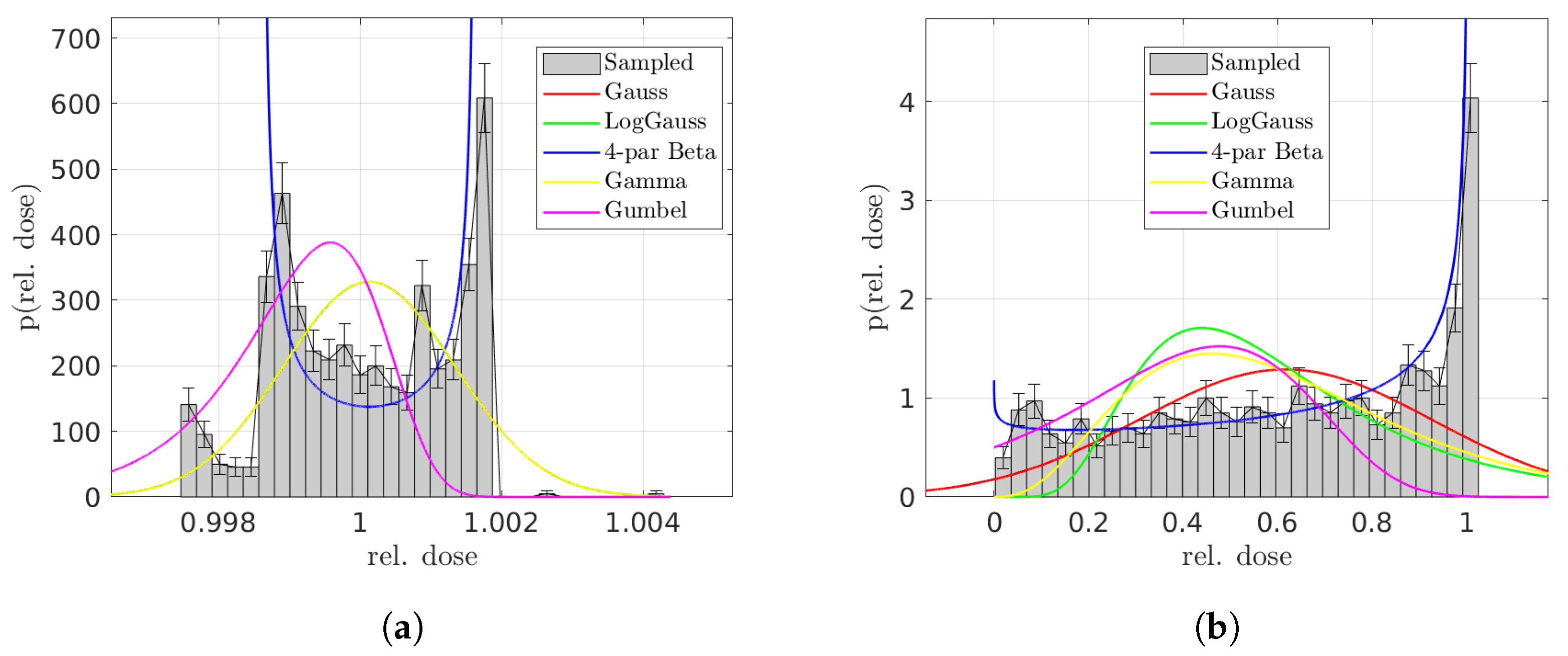
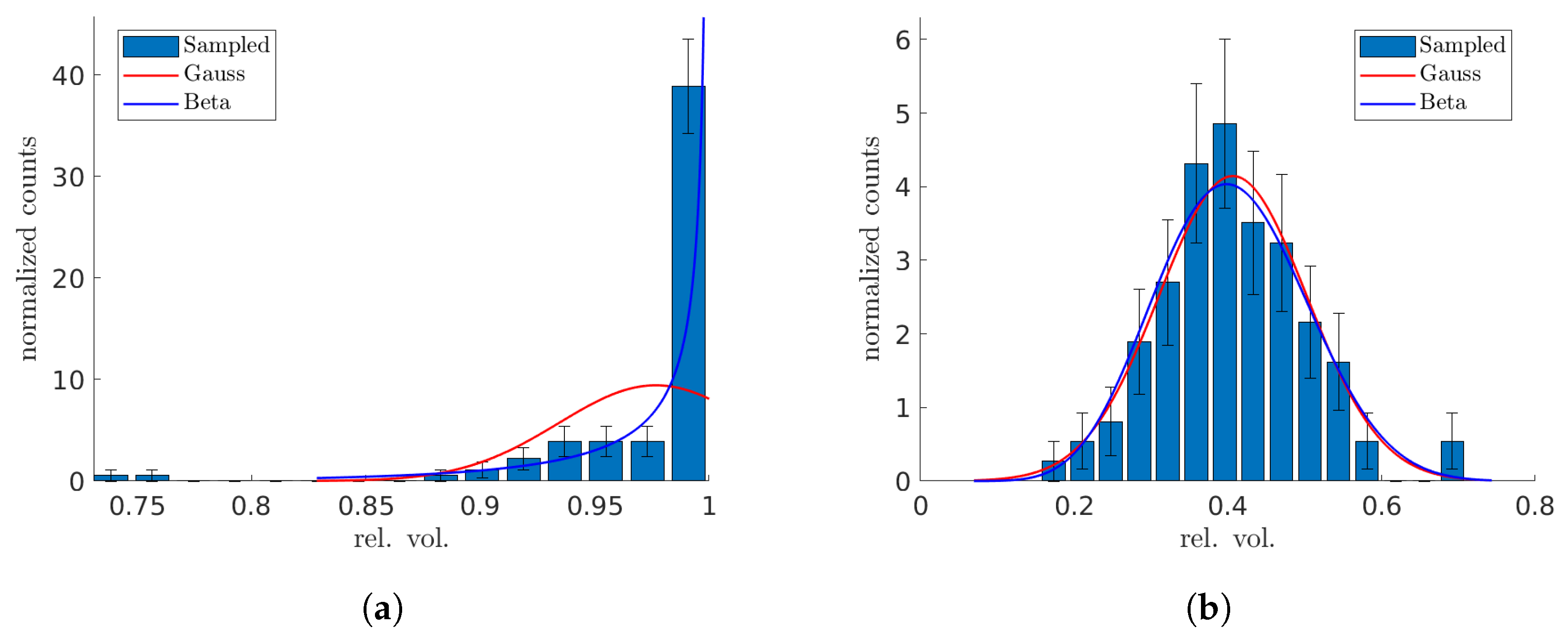
Finally, we explore the use of beta distributions for modeling Monte Carlo-sampled distributions of DVH points, and compare them with the Gaussian distributions. The rationale for considering a beta distribution is compelling: let us focus on a DVH point at a specific dose $d^{\ast }$. For a voxel within a VOI, if its dose d is greater than or equal to $d^{\ast }$ (or less than $d^{\ast }$), it is counted towards (or excluded from) the computation of the respective relative volume. This scenario can be likened to a success (or a failure) in a Bernoulli experiment. Ideally, if DVH points were independent, such a setup would naturally align with a Bernoulli process, making the beta distribution an ideal fit since it represents the probability distribution of success in this context. However, in practical terms, the voxel-based Bernoulli experiments tend to be interdependent.

2.4. Testing of the Models

Our initial evaluation of various dose-distribution assumptions is conducted using simulated DVHs on a one-dimensional prototype. This prototype is developed using the open-source “APM toolbox” [23], which facilitates the creation of simple, low-dimensional geometrical configurations for experimental purposes. The prototype’s analyzed volume extends from −50 mm to 50 mm. It includes a cancerous volume of interest (VOI) spanning from −20 mm to 20 mm, and a healthy VOI extending from 20 mm to 40 mm. The setup consists of 100 voxels, equating to one voxel per millimeter. 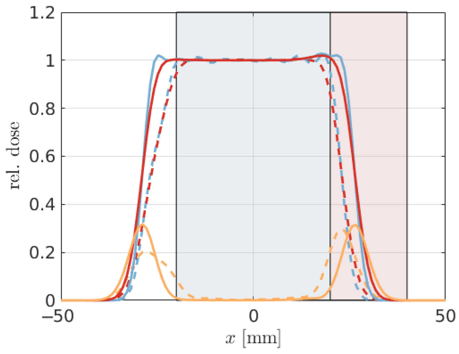A prescribed dose of $1\mathrm{Gy}$ is administered to the target VOI. In our analysis, we specifically consider the scenario where uncertainties in the pencil-beam positions are perfectly correlated, representing a realistic approximation for solid translations of the patient.

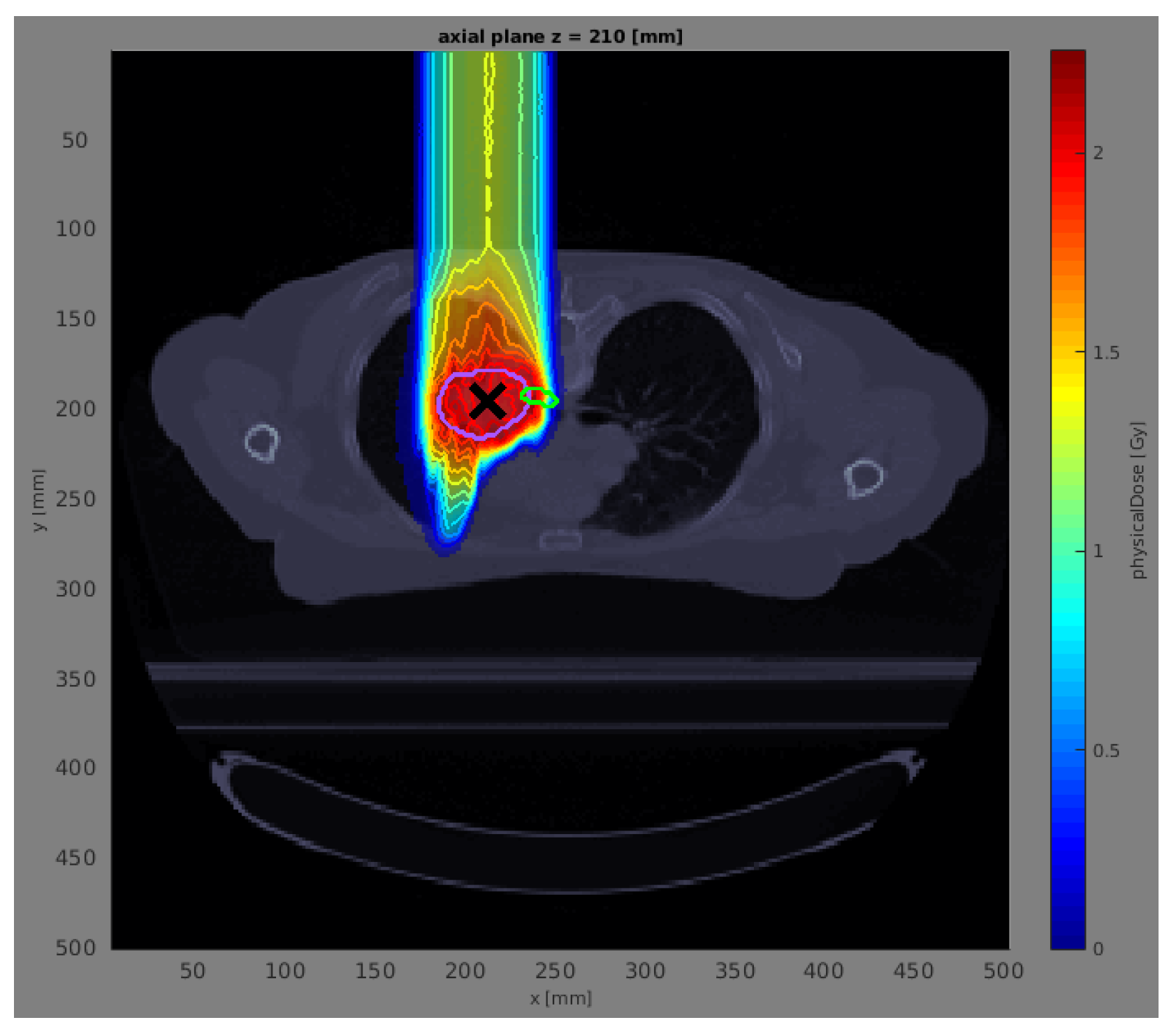
In the subsequent phase of our study, we assess the proposed models using a patient lung case treated with proton therapy. To streamline our analysis, namely, to minimize computation time and simplify the geometry, we employ a single anterior beam with a gantry angle of 0°. This approach is based on previously established reference dose distributions and corresponding error scenarios detailed in Wahl et al. [26]. These reference data were computed using the open-source radiation treatment planning software matRad [24], which allows for a comprehensive and precise evaluation within the context of proton therapy.

For the patient lung case, we additionally introduce and analyze an extra model, termed the “resampled Gaussian”. This model is derived by generating 100 random multivariate Gaussian samples of the dose, using the mean and standard deviation extracted from the Monte Carlo samples. This inclusion allows for a comprehensive comparison of the models, assessing their ability to replicate the statistical properties observed in the sampled data.

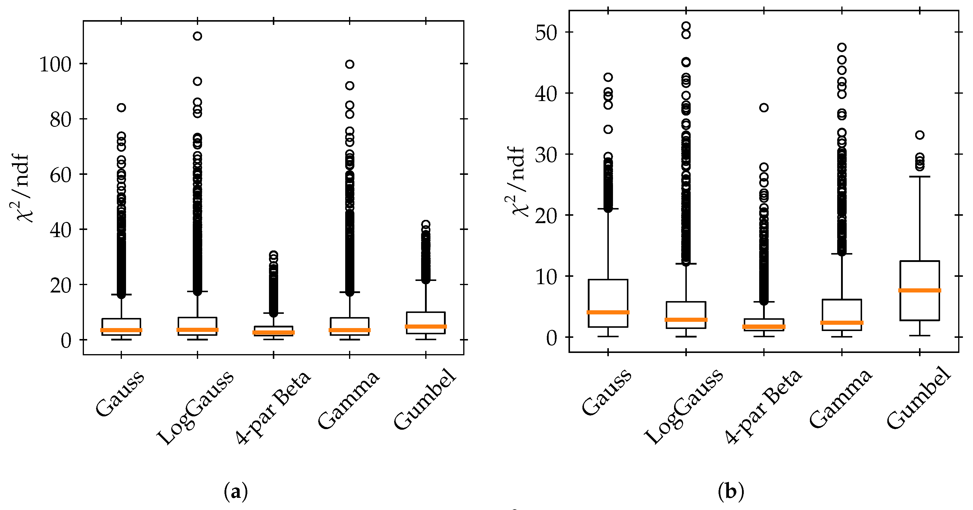
In both simulated scenarios and actual data assessments, we evaluate the accuracy of the dose uncertainty models by comparing them against Monte Carlo samples. The efficacy of the various marginal distributions in accurately representing the sampled marginal histograms is examined using Pearson’s chi-square goodness-of-fit test. The test statistic is built as

$${\chi }^2=\sum _j\frac{{\left(s_j-m_j\right)}^2}{m_j},$$

(9)

where j runs over the histogram bins, $s_j$ represents the sampled value of the histogram bin, and $m_j$ represents the modeled value. The test statistic follows approximately a ${\chi }^2$ distribution when the number of entries is large [27]. While the chi-square test is a binned approach, and thus, has certain limitations, we opt for it due to the distribution independence of its test-statistic, unlike other unbinned goodness-of-fit tests such as the Kolmogorov–Smirnov or Anderson–Darling tests. Additionally, we assess the overall impact on the DVHs by comparing the mean and standard deviation of the DVH points derived from the Monte Carlo samples with those obtained using different uncertainty models (calculated via Equation (3) and Equation (4), respectively).

3. Results

As detailed in Section 2.4, we evaluate the dose uncertainty models and their impact on dose–volume histograms; first, in the artificial one-dimensional scenario, and then, on a patient lung case.

3.1. Artificial One-Dimensional Case

Figure 1 illustrates the one-dimensional artificial geometry with two one-dimensional dose distributions for a conventionally optimized plan and a plan optimized to be robust against uncertainties. We employed a perfectly correlated, multivariate Gaussian model to represent the uncertainty in the beamlet coordinates.

The illustration reveals that probabilistic optimization more effectively encompasses the target VOI, albeit at the cost of increased dose in the healthy VOI. Notably, in the transitional region between the VOIs, the expected dose value is lower than the nominal dose for both optimization methods. This outcome underscores the robustness of the probabilistic optimization approach, demonstrating how accurately accounting for uncertainties is crucial in enhancing the quality of the treatment plan.

To determine the most suitable probability distribution for the marginal PDFs of the dose, we generated 1000 Monte Carlo samples for each voxel’s dose. Figure 2 displays the dose distributions at three distinct locations: (a) near the center of the target VOI ($x=4.5$ mm), (b) at the midpoint of the healthy VOI ($x=25.8$ mm), and (c) outside both VOIs ($x=31.8$ mm). For each scenario, Gaussian, log-normal, four-parameter beta, gamma, and Gumbel distributions are also plotted. The parameters of these distributions are not fitted; instead, they are determined using the method of moments to align the mean $\mu$ and standard deviation $\sigma$ with those of the dose at the respective voxel. Specifically, for the Gumbel distribution, the method of moments derivation is detailed in Mahdi and Cenac [28]. The minimum and maximum values for the four-parameter beta distribution are set to $max(0,\mu -1.25\sigma )$ and $\mu +1.25\sigma$, respectively, within the target VOI, and to 0 and $max(1,\mu +1.25\sigma )$ outside the target VOI and in its outermost $20\%$.

Figure 2a,b suggests that the four-parameter beta distribution better reflects the sampled dose histograms in the healthy VOI (c.f. Figure 2b). The performance of all distributions in the target VOI is nevertheless poor. It should be noted that for the majority of voxels, most distributions fail to pass a chi-square goodness-of-fit test, even at the $1\sigma$ significance level. The goodness-of-fit results can be found in more detail in Appendix A.1. The dose distribution, particularly at the center of the target VOI, exhibits a tri-modal nature, making it challenging to accurately model with two-parameter distributions, including the four-parameter beta distribution, which can only adapt to certain bi-modal distributions. This behavior is a consequence of assuming perfect correlation between beamlets. In scenarios with uncorrelated beamlets, the dose distributions at the center of the target VOI tend to resemble Gaussian distributions more closely.

The patterns observed in Figure 2 are indicative of a broader trend across the analyzed volume. Specifically, within the central span of the analyzed volume, $[-40\mathrm{mm},40\mathrm{mm}]$, most distributions fail to fit the sampled histograms, but the four-parameter beta distribution provides a more reasonable approximation of the dose distribution, specially in the healthy region. While it is not invariably the case, this distribution frequently emerges as the one minimizing the chi-square value within this central region (even if the latter is still considerably sub-optimal).

3.2. Patient Lung Case

Figure 3 shows a computer tomography scan of a publicly available lung cancer case from The Cancer Imaging Archive (TCIA), with the purple contoured internal target volume (ITV) representing the target VOI and the esophagus being a healthy VOI in green. The deposited dose is also depicted in color scale.

For the patient case, uncertainties in the positions of the beamlets were randomly sampled to generate 100 Monte Carlo samples of the dose at each voxel, as outlined in Wahl et al. [26]. Consequently, Figure 4 illustrates the sampled and modeled dose distributions for a voxel within the ITV (shown in Figure 4a) and for a voxel inside the esophagus (depicted in Figure 4b). The parameters of the distributions are determined not through fitting but by applying the method of moments to the sample mean and variance. For patient data, the bounds of the four-parameter beta distribution are set to $max(0,\mu -3\sigma )$ and $\mu +3\sigma$, with $\mu$ representing the mean and $\sigma$ the standard deviation of the dose distribution at the respective voxel.

Similar to the artificial case, we calculate the chi-square statistic for each distribution at every voxel. Although no distribution distinctly outperforms others in terms of fit, we observe the same tendency as in the one-dimensional case, i.e., the four-parameter beta distribution is mostly favored, in particular in the healthy VOI. Moreover, akin to the simulation results, the majority of distributions fail to pass the chi-square goodness-of-fit test at a $1\sigma$ significance level for most voxels. Although the goodness-of-fit results are considerably better than for the artificial case, there is still no distribution that fully captures the sampled data, as detailed in Appendix A.2. Despite this, we construct a “mix” of the most suitable marginal PDFs, selecting from the set that minimizes the chi-square test statistic at each voxel.

In order to evaluate and compare the efficacy of all the different models we tested, Figure 5 presents the absolute values (top panels) and differences to the Monte Carlo sampled values (bottom panels) in both the mean and standard deviation of the DVH points (i.e., volume fractions) as computed under each model (using Equation (3) and Equation (4) respectively).

The analysis presented in Figure 5a,b highlights that the Gaussian, gamma, and four-parameter beta distributions exhibit the smallest biases, within a range of $\pm 5\%\mathrm{vol}.$ Similarly, the resampled Gaussian model also demonstrates a minimal bias, falling within the same $\pm 5\%\mathrm{vol}.$ range. Notably, the most significant biases are observed in regions proximal to the prescribed dose value. An important observation from these results is the insensitivity of the outcomes to the choice of Copula model. This can be attributed to the fact that in the calculation of the DVH mean, as referenced in Equation (3), only the univariate marginal CDFs are utilized, which elucidates why the Copula model selection does not impact these results.

Figure 6 offers a comparative analysis between Gaussian and beta distribution models, juxtaposed with the sampled distribution of DVH points. Specifically, in Figure 6a, at a dose of $1.7\mathrm{Gy}$ for the ITV, the beta distribution clearly outperforms the Gaussian model in terms of accuracy. On the other hand, Figure 6b, depicting a dose of $1.4\mathrm{Gy}$ for the esophagus, illustrates that both Gaussian and beta distributions are viable models, albeit with some limitations. Notably, neither model consistently passes the chi-square goodness-of-fit test at the $1\sigma$ significance level. This can be appreciated in more detail in Appendix A.2. Both distributions particularly fail to reproduce the sampled distribution when the latter is heavily one-sided (typically in the target volume). Furthermore, an interesting observation is made for the DVH points of the ITV; the Gaussian model occasionally passes the chi-square test, but the residuals exhibit a discernible pattern, indicating non-randomness. This suggests that despite meeting the criteria of the goodness-of-fit test, the Gaussian model is not a good representation in this context.

4. Discussion

The primary objective of this study was to explore realistic models describing cumulative histograms arising as so-called DVHs in radiotherapy. We based our work on previous approaches relying on APM [13,14], interpreting the computation of the DVH as a series of Bernoulli experiments on uncertain dose values. With this interpretation, uni- and bivariate CDFs are required for computation of mean and variance in the DVH bins.

The integration of Copulas in constructing bivariate CDFs offers the flexibility to fuse different marginal PDFs. This approach is particularly beneficial in accurately representing the joint distribution of voxels across various sections within a volume of interest (VOI), potentially enhancing the precision (compared to the standard multivariate Gaussian [13]) and applicability of DVH models in medical physics.

Explicit modeling of uncertainty in (cumulative) histograms, including closed-form propagation from the underlying data, seems to remain an exotic task. In the search for comparable approaches, only a few published works in other fields for specialized cases could be identified. For example, Vermeesch [29] derives a frequentist and Bayesian approach to quantify uncertainties in categorical histograms as well as histograms representing time series—approaches which do not directly translate to this work. Supposedly it is often straightforward to compute “error bars” by sampling from the underlying data, or the histograms count realizations of an independent random variable, where Poisson noise may be directly assumed. In the context of radiotherapy, however, independence is not given, and the creation of a treatment plan and corresponding uncertainty modeling may be time-critical, raising the need for explicit models.

In our analysis of the one-dimensional artificial geometry, as well as of the patient lung case, the four-parameter beta distribution could improve modeling of the uncertain dose distribution across voxels within both the cancerous and healthy VOIs (more successful in the latter). This distribution, unlike the Gaussian, is capable of capturing the potentially multi-modal and skewed characteristics. However, no distribution was capable of consistently passing a goodness-of-fit test at the $1\sigma$ significance level (especially in the artificial case). The ability of the four-parameter beta distribution to describe more complex, skewed, often multi-modal dose distributions is noteworthy, but significant improvements are still needed to appropriately model the dose distributions. Considering that in the literature the only tested distribution for the dose-distributions underlying DVH computation are normal, triangular, or uniform distributions [13,30,31]—and thus, neither skewed nor multi-modal—these results constitute a first step towards a more accurate description of the dose distribution.

As a minor technical remark, the minimum and maximum values for the four-parameter beta distribution were set based on the mean ($\mu$) and standard deviation ($\sigma$) of the voxel dose distribution. The selection of these bounds for the distribution’s support was somewhat arbitrary and could be subjected to further scrutiny, yet we found that they aptly represented the simulated dose distributions.

For the patient lung case, to determine the most effective mix of distributions—that is, the combination of probability density functions (PDFs) that minimizes the chi-square test statistic at each voxel—we employed a chi-square goodness-of-fit test. However, this approach has its limitations. For instance, a distribution might exhibit a low chi-square value but still have very non-random residuals, indicating that the distribution, despite a favorable test statistic, may not be an accurate model. In other words, the process of identifying the best mix could be further refined for greater accuracy. Nevertheless, similar to our findings in the simulations, most tested distributions frequently failed the goodness-of-fit test. We suggest that even with a more optimized approach to determining the best mix, the overall impact on the results may not be substantial.

The application of Copulas allowed us to build the required bivariate CDFs from different (continuous) correlated marginal PDFs. Despite Copulas being a highly versatile approach, we found that the Copula models did not outperform the multivariate Gaussian model (or, equivalently, the model of a Gaussian Copula with Gaussian marginal PDFs). Specifically, the best mix of marginal PDFs combined with a Gaussian Copula did not demonstrate any significant advantage over the multivariate Gaussian model in accurately describing the DVH moments. DVHs derived from Gaussian resampling showed a similar pattern to those from the multivariate Gaussian model, with minor discrepancies mainly noted in the calculated standard deviation. The most effective models, exhibiting a bias within $\pm 5\%\mathrm{vol}.$ of the Monte Carlo mean for the DVH mean values, include the resampled Gaussian, and the Gaussian Copula with Gaussian, gamma, and four-parameter beta marginals, all of which approximate the standard deviation within a $\pm 10\%\mathrm{vol}.$ range. Notably, the most substantial deviations from the Monte Carlo-derived DVH mean or standard deviation were observed at the prescribed dose level. Additionally, our findings suggest that the Ali–Mikhail–Haq Copula tends to underperform relative to the Gaussian Copula, particularly in terms of underestimating the standard deviation.

In terms of generalization, the investigation of a single case in this work does not allow extrapolation to other cases. With the same irradiation setup and treatment site we may expect similar results, but the effect of changes to beam arrangements, the input uncertainty model, or anatomy cannot easily be predicted.

For example, the correlation between voxel doses is highly dependent on the correlation assumptions on the input uncertainties (i.e., patient displacement, anatomical variations, machine delivery uncertainty) [10,17]. In our simulations, we opted to model our uncertainty as patient shifts, which entails perfect correlation of all beamlets constituting a beam for irradiation. Future research may include additional sources of uncertainty, resulting in more complex correlation patterns in the input uncertainty model. Here, our approach may offer some guidance on how to represent the resulting voxel dose PDFs and CDFs and directly propagating them through the DVH calculation. Further, the APM approach allows for computation of higher moments [14], which would be beneficial to determine the shape of the marginal PDFs or covariances more accurately. However, the increased computational cost required for these calculations is currently the limiting factor prohibiting such calculations.

In an attempt to accurately represent Monte Carlo-sampled distributions of DVH points, we explored the use of the physically motivated beta distributions and compared them with the standard assumption of Gaussian distributions. As expected, the voxel-based Bernoulli experiments tended to be interdependent, which complicates the modeling process and prevents the beta distribution from being an exact fit. Despite these challenges, and the fact that the beta distribution does not consistently clear the bar of a goodness-of-fit test at the $1\sigma$ significance level, our observations indicate that it provides a better description of the distribution of sampled DVH points compared to a Gaussian model. This suggests that, while not perfect, the beta distribution offers a more nuanced and potentially more accurate representation of DVH-point distributions in our analysis.

Finally, our findings suggest that while the four-parameter beta distribution may be useful to model uncertainty in the dose distribution, their fits have not yet proven accurate enough to be employed in practice. The tested Copula models, which in this work did not outperform the bivariate Gaussian benchmark, still can constitute a straightforward way to build bivariate CDFs under different marginal PDFs, allowing us to employ specific features of the marginal probability densities in implicit modeling. For the future, considering more sources of input uncertainty and other anatomies or even in other scientific field, our work may demonstrate various modeling tools for computation of cumulative histograms from uncertain data. Another advantage, not explored in this work, is that the analytical approach of modeling these uncertainties enables, for example, the computation of derivatives. In the case of radiotherapy treatment planning, this could allow efficient optimization of dose subject to a confidence interval for a DVH point, thus rendering the treatment plan quantifiably robust (compare [32,33,34], who apply such methods using empirical DVH uncertainty estimates).

Consequently, we consider the approach itself valuable for general investigations into how uncertain data can be evaluated using probabilities in cumulative histograms.

5. Conclusions

Our study explored and compared various models for accurately describing DVH-point distributions within the context of medical physics and radiation therapy planning. While the four-parameter beta distribution showed a promising ability to capture the complexities of dose distributions within VOIs, it faced challenges in consistently passing goodness-of-fit tests (along with other tested models). The multivariate Gaussian model and its equivalent, the Gaussian Copula with Gaussian marginal PDFs, although not consistently outperforming the more complex Copula models, demonstrated reliable performance in most scenarios. Notably, the beta distribution provided a closer approximation of the Monte Carlo-sampled DVH points than the Gaussian, underscoring its potential utility despite some limitations.

This work highlights the intricate interplay between dose-distribution characteristics and the statistical models used to represent them, emphasizing the need for continued research and development of more nuanced and robust models. In particular, a better understanding of the influence that the inter-voxel correlation has in the dose distributions is clearly needed. Such advancements are crucial in enhancing the accuracy and reliability of DVH predictions, ultimately contributing to improved treatment planning and patient outcomes in radiation therapy.

References

1. Chen, H.H.W.; Kuo, M.T. Improving radiotherapy in cancer treatment: Promises and challenges. Oncotarget 2017, 8, 62742–62758. [Google Scholar] [CrossRef]
2. Malouff, T.D.; Mahajan, A.; Krishnan, S.; Beltran, C.; Seneviratne, D.S.; Trifiletti, D.M. Carbon Ion Therapy: A Modern Review of an Emerging Technology. Front. Oncol. 2020, 10, 82. [Google Scholar] [CrossRef] [PubMed]
3. Wu, Q.; Mohan, R. Algorithms and functionality of an intensity modulated radiotherapy optimization system. Med. Phys. 2000, 27, 701–711. [Google Scholar] [CrossRef] [PubMed]
4. Mayles, P.; Nahum, A.E.; Rosenwald, J.C. (Eds.) Handbook of Radiotherapy Physics: Theory and Practice; CRC Press: Boca Raton, FL, USA, 2007. [Google Scholar] [CrossRef]
5. van Herk, M.; Remeijer, P.; Lebesque, J.V. Inclusion of geometric uncertainties in treatment plan evaluation. Int. J. Radiat. Oncol. 2002, 52, 1407–1422. [Google Scholar] [CrossRef]
6. Lomax, A.J. Intensity modulated proton therapy and its sensitivity to treatment uncertainties 1: The potential effects of calculational uncertainties. Phys. Med. Biol. 2008, 53, 1027–1042. [Google Scholar] [CrossRef] [PubMed]
7. Fredriksson, A. A characterization of robust radiation therapy treatment planning methods—From expected value to worst case optimization. Med. Phys. 2012, 39, 5169–5181. [Google Scholar] [CrossRef] [PubMed]
8. Unkelbach, J.; Alber, M.; Bangert, M.; Bokrantz, R.; Chan, T.C.Y.; Deasy, J.O.; Fredriksson, A.; Gorissen, B.L.; van Herk, M.; Liu, W.; et al. Robust radiotherapy planning. Phys. Med. Biol. 2018, 63, 22TR02. [Google Scholar] [CrossRef] [PubMed]
9. Unkelbach, J.; Chan, T.C.Y.; Bortfeld, T. Accounting for range uncertainties in the optimization of intensity modulated proton therapy. Phys. Med. Biol. 2007, 52, 2755–2773. [Google Scholar] [CrossRef]
10. Wahl, N.; Hennig, P.; Wieser, H.P.; Bangert, M. Efficiency of analytical and sampling-based uncertainty propagation in intensity-modulated proton therapy. Phys. Med. Biol. 2017, 62, 5790–5807. [Google Scholar] [CrossRef]
11. Perkó, Z.; van der Voort, S.R.; van de Water, S.; Hartman, C.M.H.; Hoogeman, M.; Lathouwers, D. Fast and accurate sensitivity analysis of IMPT treatment plans using Polynomial Chaos Expansion. Phys. Med. Biol. 2016, 61, 4646–4664. [Google Scholar] [CrossRef]
12. Lowe, M.; Albertini, F.; Aitkenhead, A.; Lomax, A.J.; MacKay, R.I. Incorporating the effect of fractionation in the evaluation of proton plan robustness to setup errors. Phys. Med. Biol. 2016, 61, 413–429. [Google Scholar] [CrossRef]
13. Wahl, N.; Hennig, P.; Wieser, H.P.; Bangert, M. Analytical probabilistic modeling of dose-volume histograms. Med. Phys. 2020, 47, 5260–5273. [Google Scholar] [CrossRef] [PubMed]
14. Bangert, M.; Hennig, P.; Oelfke, U. Analytical probabilistic modeling for radiation therapy treatment planning. Phys. Med. Biol. 2013, 58, 5401–5419. [Google Scholar] [CrossRef]
15. Wieser, H.P.; Hennig, P.; Wahl, N.; Bangert, M. Analytical probabilistic modeling of RBE-weighted dose for ion therapy. Phys. Med. Biol. 2017, 62, 8959–8982. [Google Scholar] [CrossRef] [PubMed]
16. Wahl, N.; Hennig, P.; Wieser, H.P.; Bangert, M. Analytical incorporation of fractionation effects in probabilistic treatment planning for intensity-modulated proton therapy. Med. Phys. 2018, 45, 1317–1328. [Google Scholar] [CrossRef] [PubMed]
17. Wieser, H.P.; Karger, C.P.; Wahl, N.; Bangert, M. Impact of Gaussian uncertainty assumptions on probabilistic optimization in particle therapy. Phys. Med. Biol. 2020, 65, 145007. [Google Scholar] [CrossRef]
18. Stammer, P.; Burigo, L.; Jäkel, O.; Frank, M.; Wahl, N. Efficient Uncertainty Quantification for Monte Carlo Dose Calculations Using Importance (Re-)Weighting. Phys. Med. Biol. 2021, 66, 205003. [Google Scholar] [CrossRef]
19. Stammer, P.; Burigo, L.; Jäkel, O.; Frank, M.; Wahl, N. Multivariate Error Modeling and Uncertainty Quantification Using Importance (Re-)Weighting for Monte Carlo Simulations in Particle Transport. J. Comput. Phys. 2023, 473, 111725. [Google Scholar] [CrossRef]
20. Drzymala, R.E.; Mohan, R.; Brewster, L.; Chu, J.; Goitein, M.; Harms, W.; Urie, M. Dose-volume histograms. Int. J. Radiat. Oncol. 1991, 21, 71–78. [Google Scholar] [CrossRef]
21. Ali, M.M.; Mikhail, N.N.; Haq, M.S. A class of bivariate distributions including the bivariate logistic. J. Multivar. Anal. 1978, 8, 405–412. [Google Scholar] [CrossRef]
22. Nelsen, R.B. An Introduction to Copulas; Springer Series in Statistics; Springer: New York, NY, USA, 2006. [Google Scholar] [CrossRef]
23. Wahl, N.; Wieser, H.P.; Bangert, M. Analytical Probabilistic Modeling Toolbox; Deutsches Krebsforschungszentrum: Heidelberg, Germany, 2018. [Google Scholar]
24. Wieser, H.P.; Cisternas, E.; Wahl, N.; Ulrich, S.; Stadler, A.; Mescher, H.; Müller, L.R.; Klinge, T.; Gabrys, H.; Burigo, L.; et al. Development of the open-source dose calculation and optimization toolkit matRad. Med. Phys. 2017, 44, 2556–2568. [Google Scholar] [CrossRef]
25. DeGroot, M.H.; Schervish, M.J. Probability and Statistics, 4th ed.; Addison-Wesley: Boston, MA, USA, 2012. [Google Scholar]
26. Wahl, N.; Wieser, H.P.; Burigo, L.; Bangert, M. PO-1377: Monte Carlo vs. pencil-beam dose calculation for uncertainty estimation in proton therapy. Radiother. Oncol. 2020, 152, S731. [Google Scholar] [CrossRef]
27. Frodesen, A.G.; Skjeggestad, O.; Tofte, H. Probability and Statistics in Particle Physics; Universitetsforlaget: Bergen, Norway, 1979. [Google Scholar]
28. Mahdi, S.; Cenac, M. Estimating Parameters of Gumbel Distribution using the Methods of Moments, probability weighted Moments and maximum likelihood. Rev. Mat. Teor. Apl. 2012, 12, 151–156. [Google Scholar] [CrossRef]
29. Vermeesch, P. Statistical uncertainty associated with histograms in the Earth sciences. J. Geophys. Res. Solid Earth 2005, 110, B02211. [Google Scholar] [CrossRef]
30. Cutanda Henríquez, F.; Vargas Castrillón, S. The Effect of the Different Uncertainty Models in Dose Expected Volume Histogram Computation. Australas. Phys. Eng. Sci. Med. 2008, 31, 196–202. [Google Scholar] [CrossRef] [PubMed]
31. Cutanda Henríquez, F.; Vargas Castrillón, S. Confidence Intervals in Dose Volume Histogram Computation. Med. Phys. 2010, 37, 1545–1553. [Google Scholar] [CrossRef] [PubMed]
32. Gordon, J.J.; Sayah, N.; Weiss, E.; Siebers, J.V. Coverage Optimized Planning: Probabilistic Treatment Planning Based on Dose Coverage Histogram Criteria. Med. Phys. 2010, 37, 550–563. [Google Scholar] [CrossRef] [PubMed]
33. Mescher, H.; Ulrich, S.; Bangert, M. Coverage-Based Constraints for IMRT Optimization. Phys. Med. Biol. 2017, 62, N460–N473. [Google Scholar] [CrossRef]
34. Tilly, D.; Holm, Å.; Grusell, E.; Ahnesjö, A. Probabilistic Optimization of Dose Coverage in Radiotherapy. Phys. Imaging Radiat. Oncol. 2019, 10, 1–6. [Google Scholar] [CrossRef]
Figure 1. Artificial one-dimensional lateral geometry. The cancerous target VOI is shaded in blue while the healthy VOI is in red. Solid lines represent probabilistically optimized values, while dashed lines represent conventionally optimized values. In blue, we can find the nominal dose, in red the expected dose, and in yellow the standard deviation of the dose.
Stats 07 00017 g001
Figure 2. Histogram of Monte Carlo samples of the dose, and different marginal dose PDF models, for a voxel in (a) the center of the target VOI, and (b) in the center of the healthy VOI. In (a), the Gaussian, log-Gaussian, and gamma distributions overlap almost completely, such that a visual distinction is not possible.
Stats 07 00017 g002
Figure 3. Computer tomography of the lung case used in this work. The internal target volume is marked in purple and the esophagus in green. The deposited dose is shown in color scale.
Stats 07 00017 g003
Figure 4. Histogram of Monte Carlo samples of the dose, and different marginal dose PDF models, for a voxel in (a) the ITV, and (b) the esophagus. In (a), the Gaussian, log-Gaussian, and gamma distributions overlap almost completely, such that a visual distinction is not possible.
Stats 07 00017 g004
Figure 5. Comparison of the performance against Monte Carlo sampling of the different models. (a) Absolute values of the mean DVH points (top) and difference to sample mean (bottom) in the ITV. (b) Same as (a) but for the esophagus. (c) Absolute values of the standard deviation of the DVH points (top) and difference to sample standard deviation (bottom) in the ITV. (d) Same as (c) but for the esophagus. The proposed models are Gaussian resampling, or a Copula (Gaussian or Ali–Mikhail–Haq) in combination with Gaussian, log-normal, four-parameter beta, gamma, Gumbel, or a “mix” of the best-fitting marginal PDFs (see text for details).
Stats 07 00017 g005
Figure 6. Sampled and modeled distributions of a DVH point (a) in the ITV, and (b) in the esophagus. The tested models are a Gaussian and a beta distribution.
Stats 07 00017 g006
Disclaimer/Publisher’s Note: The statements, opinions and data contained in all publications are solely those of the individual author(s) and contributor(s) and not of MDPI and/or the editor(s). MDPI and/or the editor(s) disclaim responsibility for any injury to people or property resulting from any ideas, methods, instructions or products referred to in the content.