Article

Adjustment of Anticipatory Covariates in Retrospective Surveys: An Expected Likelihood Approach

by
Gebrenegus Ghilagaber
1,*,† and
Rolf Larsson
2,†
1
Department of Statistics, Stockholm University, 10691 Stockholm, Sweden
2
Department of Mathematics, Uppsala University, 75104 Uppsala, Sweden
*
Author to whom correspondence should be addressed.
These authors contributed equally to this work.
Stats 2023, 6(4), 1179-1197; https://doi.org/10.3390/stats6040074
Submission received: 30 September 2023 / Revised: 27 October 2023 / Accepted: 29 October 2023 / Published: 1 November 2023
(This article belongs to the Special Issue Advances in Probability Theory and Statistics)

Abstract

:
We address an inference issue where the value of a covariate is measured at the date of the survey but is used to explain behavior that has occurred long before the survey. This causes bias because the value of the covariate does not follow the temporal order of events. We propose an expected likelihood approach to adjust for such bias and illustrate it with data on the effects of educational level achieved by the time of marriage on risks of divorce. For individuals with anticipatory educational level (whose reported educational level was completed after marriage), conditional probabilities of having attained the reported level before marriage are computed. These are then used as weights in the expected likelihood to obtain adjusted estimates of relative risks. For our illustrative data set, the adjusted estimates of relative risks of divorce did not differ significantly from those obtained from anticipatory analysis that ignores the temporal order of events. Our results are slightly different from those in two other studies that analyzed the same data set in a Bayesian framework, though the studies are not fully comparable to each other.

1. Introduction

Consider a retrospective survey where the interest is to investigate differentials in the risk of divorce across educational levels attained before marriage, but where available information is only respondents’ highest educational level at the time of the survey. Common practice is to use the available information on educational level as a covariate in modeling the risk of divorce, an event that took place before the survey. Educational progress is likely to occur between the time of entry into marriage and the date of the survey. The questions then are, to what extent do changes in patterns of divorce across educational levels reflect real differences in divorce due to differences in educational level and what portion of these changes can be attributed to misclassification of respondents across education levels? These questions can be answered by dealing with the fact that the covariate (education) is anticipatory and adjusting the corresponding parameters to correct the bias inherent in the time inconsistency of the anticipatory covariate.
Hoem [1] warns that using anticipatory covariates is misleading, but concludes that the adverse effects may be smaller in some situations. In their study of mortality clustering in India using past births and deaths, Arulampalam and Bhalotra [2] discard anticipatory regressors: household asset, toilet facility, electricity, or access to piped water at the date of the survey. However, much valuable information may be lost by ignoring such covariates. Hoem and Kreyenfeld [3,4] argue that anticipatory covariates may provide useful information. They propose data imputation, but the procedure requires unrealistic assumptions. Faucett et al. [5] treat anticipatory covariates as missing data and their results, based on Bayesian techniques, gave interval estimates with higher coverage probabilities compared to imputation. Todesco [6] used anticipatory covariates like area of residence, education, and religious commitment to analyze marital dissolution in Italy and concluded that use of anticipatory analysis did not jeopardize the results.
Ghilagaber and Koskinen [7] and Munezero and Ghilagaber [8] used Bayesian modeling approaches and found that anticipatory analysis can lead to overestimation or underestimation of the relative risks associated with the anticipatory covariate. More recently, Hoem and Nedoluzhko [9] highlighted that use of anticipatory analysis (or “negative duration”) in estimating rates in childbearing before and after migration leads to incorrect results and should be abandoned. In a related study, Pina-Sánchez et al. [10] suggested an adjustment method based on a mixture Bayesian model in their analysis of restrospectively reported work histories in Swedish register data.
In the present study, we use a maximum likelihood approach to examine any effects of anticipatory covariates. We model divorce risks among 1312 Swedish men born between 1936 and 1964 in a piece-wise constant hazard model framework. For individuals with anticipatory educational levels, we compute conditional probabilities that these levels were attained before marriage. These probabilities are then used as weights in their contributions to the likelihood function. Adjusted relative risks of divorce across educational levels are then estimated by maximizing the weighted likelihood function. For our illustrative data set, such adjusted estimates of relative risks did not differ significantly from those obtained in the anticipatory analysis based on unweighted likelihood. The sign of the estimates is the same as in the Bayesian analysis of the same data set by Ghilagaber and Koskinen [7] and Munezero and Ghilagaber [8], but the differences between the estimates in the anticipatory and adjusted models were significant in the two previous studies [7,8].
In Section 2, we introduce the simple two-factor multiplicative model with piece-wise constant hazard and derive its likelihood function from which relevant parameters are estimated. We extend this standard likelihood function to a weighted likelihood function in Section 3 and derive the corresponding parameter estimates. In Section 4, we illustrate our proposed approach using data on the effect of anticipatory educational level on divorce risks among Swedish men. We summarize our findings in Section 5 by way of concluding remarks and suggestions for future investigations. An appendix contains omitted derivations as well as tables and figures of of our empirical findings.

2. The Multiplicative Two-Factor Hazard Model

For a sample of individuals, consider J educational levels and let D i j be the number of divorces at marriage duration i ,   i = 1 , , I and education level j ,   j = 1 , , J for T i j years of observed exposure to the risk of divorce. The covariate indexed by i is the grouped-time variable (duration of marriage) measured from the date of marriage until the date of divorce or until the interview date, whichever comes first.
Define
D i + = j = 1 J D i j , D + j = i = 1 I D i j ,
D + + = i = 1 I D i + = j = 1 J D + j = i = 1 I j = 1 J D i j ,
and let T i + ,   T + j , and T + + represent similar quantities for the exposure variable T. Divorce risks are assumed to be piece-wise constant in each of the the I time intervals, but may vary between intervals. The time to divorce then follows a piece-wise exponential distribution for each educational level. The density function of the time to divorce in duration group i for a person k with educational level j is then given by
f ( t i j k ) = λ i j exp λ i j t i j k .
A multiplicative model for the hazard rate λ i j [11,12] corresponds to
λ i j = β i α j ,
where β i is the baseline risk of divorce at marriage-duration i and α j is the relative risk of divorce for individuals with education level j (relative to those with the educational level that is used as the baseline/reference).
The model in Equation (4) has I + J parameters β 1 , β 2 , , β I and α 1 , α 3 , , α J . To construct the likelihood function when Equation (4) holds, we define δ i j k as an indicator of whether the kth sample member having the jth level of education is divorced ( δ i j k = 1 ) or is still married ( δ i j k = 0 ) in the ith marriage-duration. From Equations (3) and (4), the contribution to the likelihood of the n i j sub-sample of individuals in the ith marriage-duration and having the jth level of education, is obtained as
Λ i j = k = 1 n i j β i α j δ i j k exp β i α j t i j k = β i α j D i j exp β i α j T i j ,
where
D i j = k = 1 n i j D i j k and T i j = k = 1 n i j t i j k .
The likelihood for the entire sample is then the product of the Λ i j over all levels of i and j:
Λ = i = 1 I j = 1 J Λ i j = i = 1 I j = 1 J β i α j D i j exp β i α j T i j ,
so that
ln Λ = i = 1 I j = 1 J D i j ln β i α j i = 1 I j = 1 J β i α j T i j = i = 1 I j = 1 J D i j ln β i + i = 1 I j = 1 J D i j ln α j i = 1 I j = 1 J β i α j T i j = i = 1 I D i + ln β i + j = 1 J D + j ln α j i = 1 I j = 1 J β i α j T i j .
Differentiating ln Λ in Equation (7) with respect to β i and, separately, with respect to α j , equating the resulting derivatives to 0, and solving for the unknown parameters leads to the following equations
β i * = D i + j = 1 J α j * T i j , i = 1 , 2 , , I
and
α j * = D + j i = 1 I β i * T i j , j = 1 , , J .
This system of I + J equations has no analytical solution in general, but can be solved iteratively using numerical methods.

3. Adjusting for Anticipatory Covariates

3.1. Expected Likelihood

From Equations (8) and (9), we note that the maximum likelihood estimates of the baseline hazards β ^ i and relative hazards α ^ j are functions of the total number of events, D i j , and exposure times, T i j . Therefore, misclassification of events or exposure times into wrong intervals or into wrong levels of the covariate, as with anticipatory covariates, can lead to incorrect estimates of the parameters.
Consider those individuals who have completed their reported highest educational level after marriage. Inference is based on the individuals’ education levels at the date of marriage, but only their highest level of education at the date of interview is observed. This is an incomplete data problem, which is handled by maximizing the expected likelihood, conditional on available information [13].
Equation (3) denotes the density conditional on the level of education x k T k for individual k at the age of marriage T k . Since we are interested on when the reported educational level j was completed (before or after marriage), j = j k , the unconditional density is given by
g t i j k = f t i j k P x k T k = j k .
We also impose the distribution P x k T k = j k , which adds a term to the log-likelihood:
ln Λ ˜ = ln Λ + k = 1 n i j ln P x k T k = j k ,
where ln Λ is as in Equation (7), and the last term in Equation (11) reflects contribution, to the likelihood function, of the distributions of times to educational progress (time to complete primary level, time between primary- and secondary-levels, and time between secondary- and post-secondary levels).

3.2. Parameter Estimation in the Expected Likelihood

To calculate the components of the last term, k = 1 n i j ln P x k T k = j k , in Equation (11), assume that J = 3 and, as in [7,8], let S j k denote the time of transition from educational level j 1 to educational level j for individual k, let f j denote the density function of S j k , and let F j denote its distribution function. We introduce Bernoulli variables Z j of parameters ϕ j as indicators of whether or not the level x k T k = j is the highest educational level. Then, ruling out the possibility that x k T k = 0 leads to Proposition 1.
Proposition 1.
Writing p j k P x k T k = j ,
p 1 k = F 1 T k 1 ϕ 1 0 T k f 1 u F 2 T k u d u , p 2 k = 0 T k f 1 u F 2 T k u d u 1 ϕ 2 u = 0 T k f 1 u v = 0 T k u f 2 v F 3 T k u v d v d u , p 3 k = u = 0 T k f 1 u v = 0 T k u f 2 v F 3 T k u v d v d u .
Proof. 
See Appendix A.1. □
To calculate all P x k T k = j explicitly, distributions are imposed on the times, S j k , spent at the different educational levels. As in [7,8], a piece-wise gamma distribution with density function
f j s = η j ζ j s ζ j 1 Γ ζ j exp η j s ,
and distribution function
F j s = Γ ζ j , η j s ,
is assumed, where
Γ a , s = 0 s u a 1 Γ a exp u d u
is the incomplete gamma function.
Writing
E * · = E · | y 1 , , y K ,
Equations (7) and (11) lead to
E * ln Λ ˜ = i = 1 I E * D i + ln β i + j = 1 J E * D + j ln α j i = 1 I j = 1 J E * T i j β i α j + k E * ln P x k T k = j k .
To make inference on the parameters β i and α j , the conditional expectations of the sufficient statistics D i + , D + j , and T i j need to be calculated. We re-write
D i + = k = 1 n i j D i j k I k A i , D + j = k = 1 n i j D i j k I k B j , T i j = k = 1 n i j t i j k I k A i B j = k = 1 n i j l i min t l j k m l , m l + 1 m l I k A i B j ,
where A i is the set of individuals with common first index i, B j is the set of individuals with common second index j, m i is the lower duration limit in group i , and I A is the indicator function of the event A. For each individual k, only one marriage duration group i = i ( k ) and one educational level j = j k are observed. However, if that educational level is completed after marriage, the educational level at time of marriage is unknown. By introducing distributional assumptions on time to complete a certain educational level, the probabilities are calculated as
P j k = j 0 | y k = P x k T k = j 0 | x k t k = y k ,
where t k is the age at completion of the reported level of education for individual k. This feature does not affect D i + , since summation is over j. However, it affects D + j and T i j , since different individuals may belong to different B j depending on their unknown education level at time of marriage.
Hence, we need to compute
E D + j | y 1 , , y K = k E D i j k I k B j | y k .
Re-writing the right-hand side as
E D i j k I k B j | y k = D i j k P k B j | y k
= D i j k P x k T k = j | x k t k = y k ,
gives
E D + j | y 1 , , y K = k = 1 n i j D i j k P x k T k = j | x k t k = y k .
Similarly,
E T i j | y 1 , , y K = k = 1 n i j l i E min t l j k m l , m l + 1 m l I k A i B j | y k = k = 1 n i j l i min t l j k m l , m l + 1 m l I k A i P x k T k = j | x k t k = y k .
In order to maximize the adjusted log-likelihood in Equation (11) over the parameters β i and α j , we first plug in the expression in Equation (22) into Equation (9) and the expression in Equation (23) into Equations (8) and (9), and proceed in the usual manner.
To make inference on ζ j , η j , and ϕ j , note first that (see Equation (11))
k = 1 n i j E ln P x k T k = j k | y k = k = 1 n i j j = 1 J ln P x k T k = j P x k T k = j | x k t k = y k .
Each set of ζ j , η j , and ϕ j values produces a numerical value of Equation (24) as well as expected values of the sufficient statistics in Equations (22) and (23), which, in turn, are used to maximize ln Λ ˜ in Equation (11).
This way, the expected log-likelihood for any set of ζ j , η j , and ϕ j is calculated and maximized with respect to the α j and β i parameters.
The next step is to maximize over ζ j , η j , and ϕ j using the Newton–Raphson algorithm. According to Orchard and Woodbury [13], such a procedure yields the desired maximum likelihood estimates. The values of the P x k T k = j , x k t k = y are obtained using Proposition 2.
Proposition 2.
Writing p j y k P x k T k = j , x k t k = y leads to
p 11 k = F 1 T k 1 ϕ 1 0 T k f 1 u F 2 t k u d u , p 12 k = 1 ϕ 1 0 T k f 1 u F 2 t k u F 2 T k u d u 1 ϕ 2 u = 0 T k f 1 u v = T k u t k u f 2 v F 3 t k u v d v d u , p 22 k = 0 T k f 1 u F 2 T k u d u 1 ϕ 2 u = 0 T k f 1 u v = 0 T k u f 2 v F 3 t k u v d v d u , p 13 k = p 1 k p 11 k p 12 k , p 23 k = p 2 k p 22 k , p 33 k = p 3 k .
Proof. 
See Appendix A.2. □
Then, the P x k t k = y are expressed in terms of the probabilities in Equation (25) to get
P x k t k = 1 = P x k T k = 1 , x k t k = 1 ,
P x k t k = 2 = P x k T k = 1 , x k t k = 2 + P x k T k = 2 , x k t k = 2 ,
and
P x k t k = 3 = P x k T k = 1 , x k t k = 3 + P x k T k = 2 , x k t k = 3 + P x k T k = 3 , x k t k = 3 .

4. Illustration: Effect of Education on Divorce

4.1. Data set

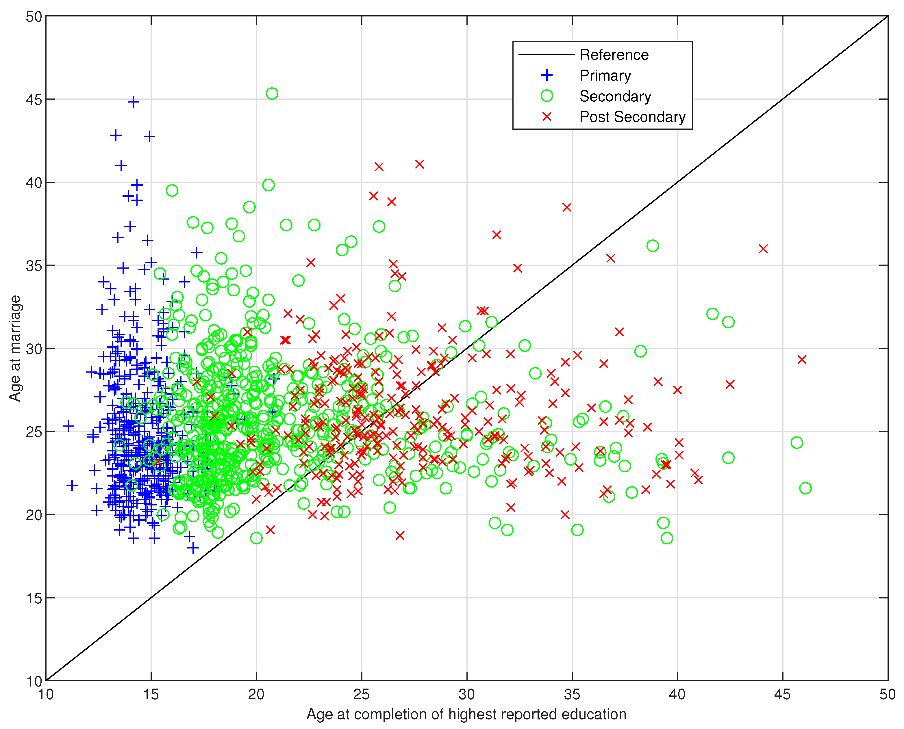
An extract from the 1985 Mail Survey of Swedish men is used as our data for illustration. The survey contained background variables as well as retrospective information on entry into and exit from marital and non-marital unions. Analysis is based on 1312 ever-married men who were either divorced or still married by the survey time. Their distribution across age at marriage and age at attainment of the reported educational level is shown in Figure A1. Those below the diagonal are the 245 (19%) observations whose reported educational level was completed after they married. Anticipatory analysis, common in the analysis of such types of data, amounts to moving the values below the diagonal in Figure A1 to the left—all the way to the diagonal reference line. A cross tabulation of the sample, as displayed in Table A1, shows differentials in percentage divorced across the anticipatory status of education. The main goal of our work is investigating the role of misclassification on such differentials in educational gradients of divorce.

4.2. Models

The time variable, duration of marriage in years, is categorized into five intervals: 0–1 , 1–2 , 2–3 , 3–6 , and 6 + years. Primary level of education is used as baseline level and, hence, its corresponding relative hazard, α 1 , is set to 1 . To make the proposed adjustment comparable to previous works on the same data set [7,8], the parameters from the common anticipatory approach and from a reduced model are also estimated. Using anticipatory analysis amounts to “back-dating” the times of highest educational achievement, τ k , for a number of individuals, while, in the reduced model, observations whose reported educational level was completed after marriage, T k < t k , are discarded.
Neither the anticipatory manipulations nor the proposed adjustment change the observed marginal occurrences D i + and exposures T i + . In the reduced model, these marginals are reduced due to the reduction of the total number of respondents. The time at which the highest educational level is achieved is irrelevant as long as it precedes the time of marriage, but it is relevant for calculating exposure times whenever it occurs after the time of marriage.
The conditions required for using the Fisher information to construct confidence intervals may not be fulfilled, due to the nature of the problem at hand. Instead, the bootstrap method is used. The individuals are bootstrapped B times and the expected likelihood for each such sample is maximized. We then calculate empirical 95% confidence intervals for each parameter by computing the 2.5 % and 97.5 % percentiles of the bootstrap distributions. An alternative approach is to compute standard deviations and form normal approximation confidence intervals. But, this approach was considered problematic because of outliers in the bootstrap distributions. In the reduced and anticipatory cases, the number of bootstrap replications were B = 10,000. In the adjusted case, B = 1000 because estimation of the additional parameters ζ and η required heavy computation. In the bootstrap replications, integrals and derivatives were calculated in the same manner as in the estimation. The estimated parameters were taken as starting values for each bootstrap replication.

4.3. Numerical Considerations

Numerical integration was used to calculate the integrals for given parameter values. When maximizing the expected likelihood over the ϕ parameters, one problem may arise. All the P x T = j are linear in the ϕ i and, hence, for individuals with t k T k , the derivatives of ln P x k T k = j k may be non-zero for all possible ϕ i . Hence, if all individuals would have t k T k , and, thus, conditioning would be unnecessary, the likelihood may be maximized at the boundary of the parameter space, ϕ i = 0 or ϕ i = 1 , for i = 1 and 2 . These solutions might be considered unrealistic. For individuals with T k < t k , the situation is less clear-cut, but if the majority of the individuals have t k T k , there is a risk that their contribution dominates the likelihood, and this seems to be the case in the data set used for our illustration.
Hence, the ϕ i parameters were fixed to the empirical proportions of men who did not continue to the next higher level (see Table A1). We assigned ϕ 1   = 0.34 , obtained from Table A1 as 442 1312 , and ϕ 2 = 0.66 , obtained from Table A1 as 488 + 94 1312 442 . These are also almost identical to the Bayesian estimates obtained in [7,8].
Instead of considering the gamma distribution parameters ζ j , η j explicitly in the maximization, it was more convenient to use the transformed parameters μ j = ζ j η j and σ j = ζ j 1 2 η j . These correspond to the expectations and standard deviations, respectively. We found that the likelihood has an asymptote as σ 3 0 . To alleviate this problem, σ 3 was fixed and maximization was carried over the other parameters. This turned out to work out well. Unlike the ϕ parameter, there was no natural choice of ad hoc value of σ 3 . However, the maximum with respect to all other parameters, including α j and β i , was very robust to different choices. We decided to put σ 3 = 0.5 , which seemed to be a reasonable value.
To obtain the maximum of the expected likelihood, several methods were combined. Each likelihood calculation was performed for a fixed set of the five gamma distribution parameters, μ 1 ,   μ 2 ,   μ 3 ,   σ 1 , and σ 2 , including a maximization with respect to the α j and β i parameters. Thus, in principle, the required task was to maximize over the gamma parameters. Initially, a random choice of parameter values was performed, and the ones that gave the largest value of the likelihood were selected. Then, using the Newton–Raphson maximization algorithm, the likelihood was maximized over the five gamma distribution parameters, one at a time, keeping the others fixed. Finally, we maximized over μ 1 ,   μ 2 ,   μ 3 ,   σ 1 , and σ 2 simultaneously, using the Newton–Raphson maximization algorithm in five dimensions.
To obtain approximate confidence intervals for the parameters, a bootstrap procedure was used to sample the individuals with replacement. We performed the maximization procedure described above for each bootstrap replication. While bootstrapping, the μ 3 parameter drifted towards zero in about 6 % of the bootstrap replications during the Newton–Raphson iterations. As a negative value of μ 3 is not reasonable, an extra condition, μ 3 0.001 , was imposed to overcome the problem. Further details on numerical issues, including Matlab codes, can be obtained from the authors upon request.

4.4. Results

4.4.1. Conditional Probabilities

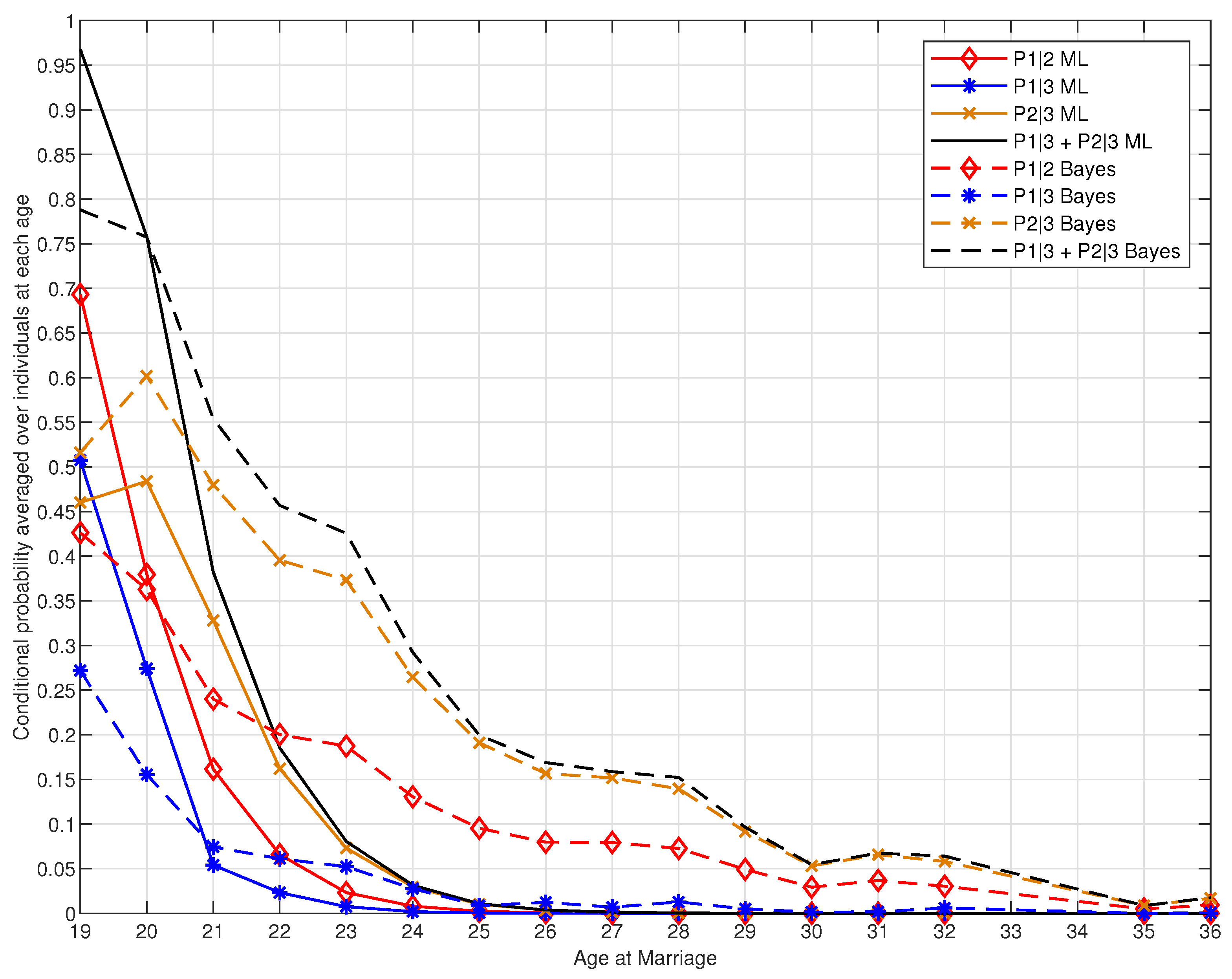
Figure A2 displays the distribution of conditional probabilities of various educational levels at marriage, given a corresponding reported educational level at time of survey, based on the 245 individuals who have completed their reported educational level after marriage. For comparison purposes, corresponding conditional probabilities computed by using estimates of the covariate-model parameters in a Bayesian analysis of the same data set [7] are also plotted.
The plots show that the probabilities of having had a lower educational level at marriage, given some higher level at interview, decrease with age at marriage. Thus, for someone who reports a post-secondary educational level at interview but has married early, say, below age 20, the probability that he had primary-level education at marriage, P 1 | 3 , is almost 1 (see Figure A2). The probability that he had secondary-level education at marriage, P 2 | 3 , is also high, but not as high as P 1 | 3 . The combined probability that he had a lower-level education, primary or secondary, is almost 1.
A comparison of the ML- and Bayes-estimates of the conditional probabilities indicates that the Bayes-estimates are, in general, higher than their corresponding ML-estimates. This is especially the case at older ages of marriage and for men who reported post-secondary-level of education at time of survey.

4.4.2. Model Parameters

Table A2 contains estimates of baseline risks, β i expressed per 1000 exposure units, and relative risks of divorce, α j , across the three models, together with their corresponding 95% confidence intervals. Except for the effect of the second interval, β 2 , which is much lower in the reduced model, the estimates of the baseline risks, β i , are close to each other across the three models.
The estimates of the relative risks α j , on the other hand, vary appreciably across models. For instance, men with secondary-level education have about the same risk of divorce as those with primary level education in the reduced model, 10 % higher risk in the anticipatory model, and a negligible 5 % higher risk in the adjusted model. Those with post-secondary education have much higher risks of divorce relative to the baseline men with primary education. The excess risk is 57 % in the reduced model, 35 % in the anticipatory model, and 34 % in the adjusted model.
More interesting for the present purpose are differences in the estimates of relative risks across the models. That the anticipatory model leads to the same estimates of the relative risks, α j , as in the adjusted model ( 1.13 and 1.05 for α 2 ;   1.35 and 1.34 for α 3 ) indicates that anticipatory analysis is harmless in our data, in the sense that it does not lead to substantial bias in the estimates of the relative risks. These estimates of relative risks are somewhat higher than those obtained by Bayesian adjustment by of the same data set [7]. This is especially true for the estimate of α 3 , but it should be borne in mind that the 95 % confidence intervals for α 2 and α 3 in both the current study and those based on Bayesian approach include 1 and, hence, are not significant at 5 % significance level. Further, a re-estimation of α 3 using the Bayes-estimated parameters of the gamma distribution yielded α ^ 3 = 1.30 , which is almost identical to the α ^ 3 = 1.34 obtained through the maximum likelihood approach.
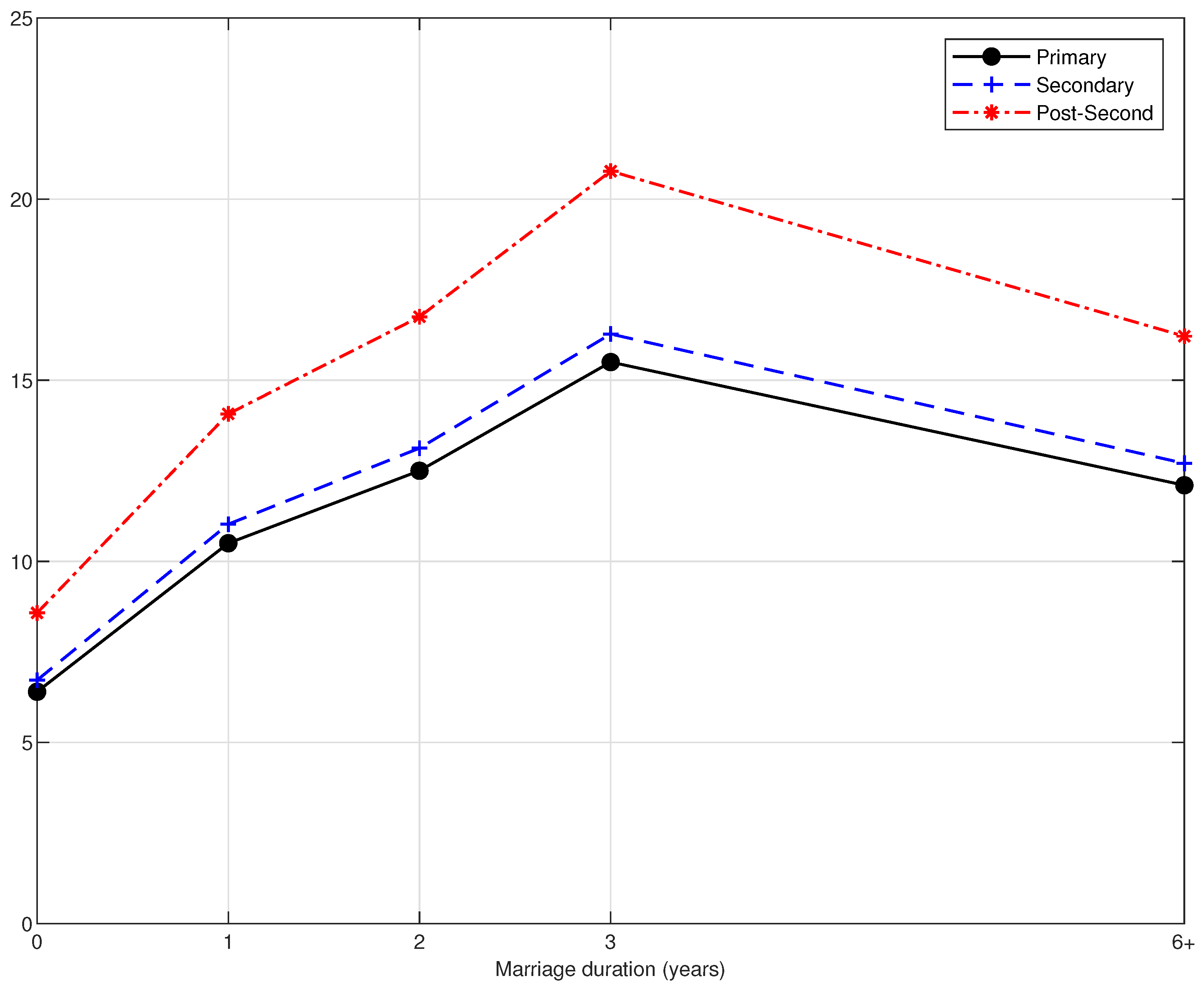
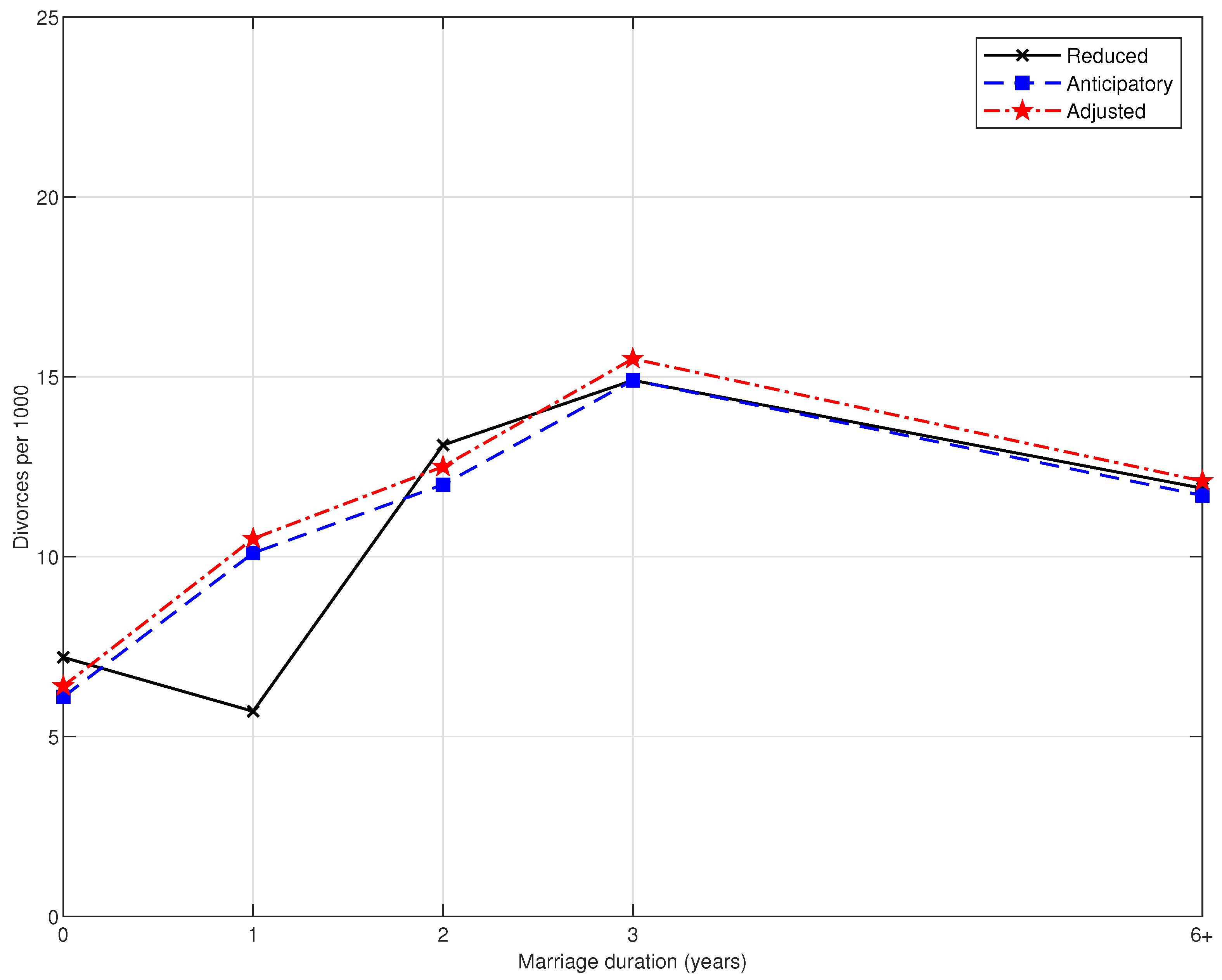
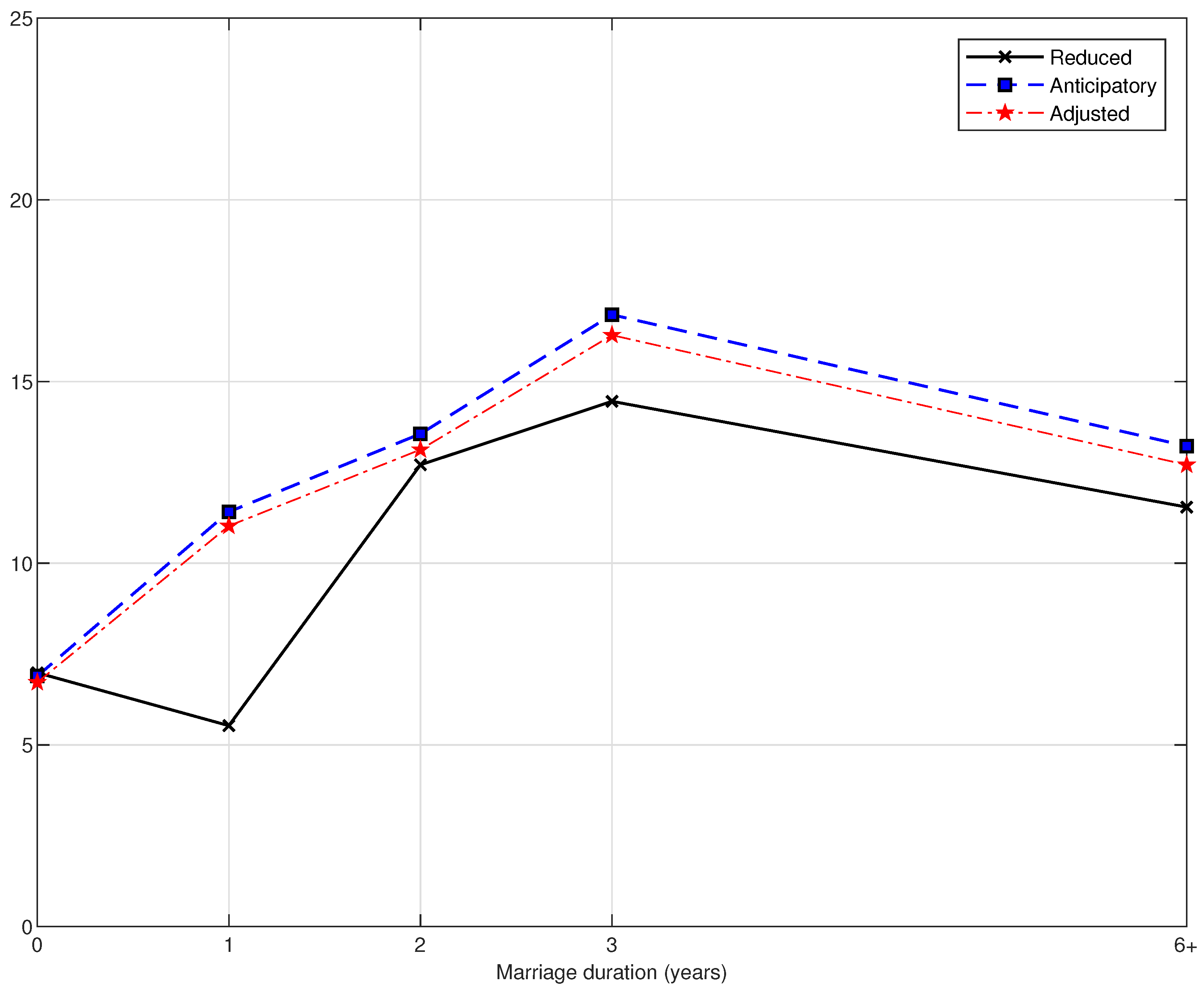
The combined effects of the differences in the estimates of the model parameters, β i and α j , across the three models and for the three educational levels are depicted in Figure A3, Figure A4, Figure A5, Figure A6, Figure A7, Figure A8, which contain estimates λ ^ i j = β ^ i α ^ j under various configurations. Figure A3, Figure A4, Figure A5, show educational profiles of divorce risks over marriage durations for each of the three models (reduced, anticipatory, and adjusted). In Figure A6, Figure A7, Figure A8, differences in the estimates of divorce risks across the three models are depicted for each educational level (primary, secondary, and post-secondary). Divorce risks increase over the first four time intervals, except in the reduced model, which exhibits decrease in the risk between first and second interval, and decrease after about 6 years (Figure A3, Figure A4, Figure A5). Further, the levels and trends are alike across the anticipatory and adjusted models (Figure A6, Figure A7, Figure A8).

4.4.3. Covariate-Model Parameters

In the adjusted model, the parameters of the gamma-distribution for educational career, ζ j and η j , are also estimated, in addition to the model parameters β i and α j . These are shown in the lower half of the last column in Table A2. These parameters are then used to compute estimates of the expected duration to complete the various educational levels, as displayed in Table A3. Thus, it takes, on average, 16.4 years after birth to complete primary-level education, 3.6 years to complete secondary-level education after completing primary level, and 1.9 years to complete post-secondary-level education after completing secondary level. The corresponding figures from the Bayesian analysis, extracted from the estimates in [7], were 14.8 , 6.5 , and 6.3 years., while those in [8] were 3.56 years to complete secondary-level education (after completing primary level) and 2.43 years to complete post-secondary-level education (after completing secondary-level education). The Bayesian-based estimates differ much from our current expected-likelihood-based estimates. However, as can be seen in Table A5, where estimates of the model parameters α j and β i , given the Bayesian estimates of the gamma-distribution parameters, are presented, it is easy to observe, by comparing to Table A2, that the estimates of the model-parameters from our expected likelihood approach are very robust to this kind of changes in the gamma parameters.
In Table A3 and Table A4, in addition to estimates of means μ j and standard deviations σ j of education times, 80 % bootstrap confidence intervals are also presented. The reason behind choosing 80 % instead of 95 % is due to problems in estimating μ 3 as already described in Section 4.4. No confidence interval is provided for σ 3 because it was fixed to 0.5 . This might also have contributed towards the relatively narrow confidence intervals for ζ 3 and η 3 in Table A2.
Finally, in Table A6, the results from our adjusted model in Table A2 are presented together with corresponding results from previous studies—Ghilagaber and Koskinen (G & K) [7] and Munezero and Ghilagaber, (M & G) [8] for comparison purposes. Our results show that anticipatory analysis is harmless because it leads to the same conclusion as the adjusted model. In the two previous studies, however, the conclusions from the respective adjusted models were different, at least partly, from those based on anticipatory analysis. However, the differences between the results in the adjusted and the anticipatory models were in opposite directions in the two previous studies. While results in [7] show that anticipatory analysis leads to overestimation of the relative risk of divorce for those with post-secondary education, results in [8] show that it leads to underestimation of the relative risks for the same group of individuals. But, it is worth noting that the three studies are not comparable to each other (even the two that use Bayesian methods) because they use different approaches and the results are presented using different baseline levels (though we transformed the relatives risks from previous to have the same baseline as ours in Table A6).

5. Summary and Concluding Remarks

In this study, we addressed a problem in inference, where the value of a covariate is measured at the date of the survey but is used to explain behavior that has occurred long before the survey.
To correct for bias due to the lack of temporal order of events, we proposed an expected likelihood approach, where conditional probabilities of having attained the reported level before marriage were computed and used as weights in the likelihood. Adjusted relative hazards were then estimated by maximizing the expected likelihood which, in turn, was based on some distributions for the time to complete various educational levels.
Our proposed analytic procedure was illustrated with data on the effects of educational level achieved at time of marriage on risks of divorce. Our results showed that anticipatory analysis is harmless because the adjusted estimates of relative risks are close to those from anticipatory analysis.
Whether such results can be replicated on other data sets or on the same data set but with different events of interest, like family formation, through cohabitation or marriage, or childbearing, is an open question for future investigation.
Further, our results are slightly different from two other studies that analyzed the same data set in a Bayesian framework.
Thus, further studies that examine the effects of anticipatory analyses more deeply are needed. Such studies can, for instance, use simulated data in order to draw stronger conclusions about the behaviour of anticipatory analysis under various data configurations.

Author Contributions

Conceptualization, G.G. and R.L.; methodology, G.G. and R.L.; software, R.L.; validation, G.G. and R.L.; formal analysis, G.G. and R.L.; investigation, G.G. and R.L.; resources, G.G. and R.L.; data curation, G.G.; writing—original draft preparation, G.G. and R.L.; writing—review and editing, G.G. and R.L.; visualization, G.G. and R.L.; supervision, G.G. and R.L.; project administration, G.G. All authors have read and agreed to the published version of the manuscript.

Funding

This research received no external funding.

Institutional Review Board Statement

Not applicable.

Informed Consent Statement

Not applicable.

Data Availability Statement

Not applicable.

Acknowledgments

A draft version of this article [14] has been presented in the regular seminars at the Departments of Statistics at Stockholm and Uppsala Universities. We are grateful to participants at those occasions as well as three anonymous referees for their valuable comments that improved the paper substantially.

Conflicts of Interest

The authors declare no conflict of interest.

Appendix A. Omitted Proofs & Tables and Figures of Empirical Results

Appendix A.1. Proof of Proposition 1

We find (dropping the index k for ease of exposition)
p 1 = P x T = 1 = 1 ϕ 1 P x T = 1 | Z 1 = 0 + ϕ 1 P x T = 1 | Z 1 = 1 = 1 ϕ 1 P S 1 T , S 1 + S 2 > T + ϕ 1 P S 1 T = 1 ϕ 1 0 T f 1 u 1 F 2 T u d u + ϕ 1 F 1 T = F 1 T 1 ϕ 1 0 T f 1 u F 2 T u d u ,
and, similarly,
p 2 = P x T = 2 = 1 ϕ 2 P x T = 2 | Z 2 = 0 + ϕ 2 P x T = 2 | Z 2 = 1 = 1 ϕ 2 P S 1 + S 2 T , S 1 + S 2 + S 3 > T + ϕ 2 P S 1 + S 2 T = 1 ϕ 2 u = 0 T f 1 u v = 0 T u f 2 v 1 F 3 T u v d v d u + ϕ 2 0 T f 1 u F 2 T u d u = 0 T f 1 u F 2 T u d u 1 ϕ 2 u = 0 T f 1 u v = 0 T u f 2 v F 3 T u v d v d u ,
while
p 3 = P x T = 3 = P S 1 + S 2 + S 3 T = u = 0 T f 1 u v = 0 T u f 2 v F 3 T u v d v d u .

Appendix A.2. Proof of Proposition 2

We obtain (by dropping the index k for ease of exposition)
p 11 = P x T = 1 , x t = 1 = 1 ϕ 1 P x T = 1 , x t = 1 | Z 1 = 0 + ϕ 1 P x T = 1 , x t = 1 | Z 1 = 1 = 1 ϕ 1 P S 1 T , S 1 + S 2 > t + ϕ 1 P S 1 T = 1 ϕ 1 0 T f 1 u 1 F 2 t u d u + ϕ 1 F 1 T = F 1 T 1 ϕ 1 0 T f 1 u F 2 t u d u ,
and
p 12 = P x T = 1 , x t = 2 = 1 ϕ 1 1 ϕ 2 P x T = 1 , x t = 2 | Z 1 = 0 , Z 2 = 0 + 1 ϕ 1 ϕ 2 P x T = 1 , x t = 2 | Z 1 = 0 , Z 2 = 1 + ϕ 1 P x T = 1 , x t = 2 | Z 1 = 1 = 1 ϕ 1 1 ϕ 2 P S 1 T , T < S 1 + S 2 t , S 1 + S 2 + S 3 > t + 1 ϕ 1 ϕ 2 P S 1 T , T < S 1 + S 2 t + 0 = 1 ϕ 1 1 ϕ 2 u = 0 T f 1 u v = T u t u f 2 v 1 F 3 t u v d v d u + 1 ϕ 1 ϕ 2 0 T f 1 u F 2 t u F 2 T u d u = 1 ϕ 1 0 T f 1 u F 2 t u F 2 T u d u 1 ϕ 1 1 ϕ 2 u = 0 T f 1 u v = T u t u f 2 v F 3 t u v d v d u .
Moreover,
p 22 = P x T = 2 , x t = 2 = 1 ϕ 2 P x T = 2 , x t = 2 | Z 2 = 0 + ϕ 2 P x T = 2 , x t = 2 | Z 2 = 1 = 1 ϕ 2 P S 1 + S 2 T , S 1 + S 2 + S 3 > t + ϕ 2 P S 1 + S 2 T = 1 ϕ 2 u = 0 T f 1 u v = 0 T u f 2 v 1 F 3 t u v d v d u + ϕ 2 0 T f 1 u F 2 T u d u = 0 T f 1 u F 2 T u d u 1 ϕ 2 u = 0 T f 1 u v = 0 T u f 2 v F 3 t u v d v d u ,
and the rest of the equalities are trivial.

Appendix A.3. Tables and Figures of Empirical Results

Table A1. Distribution of the sample of 1312 Swedish men across anticipatory status of education and status of marriage.
Status
Still MarriedDivorcedTotal% Divorced
Non-AnticipPrimary3717144216
Secondary4335548811
Post Secon.1162113715
920147106714
AnticipatoryPrimary----
Secondary66289430
Post-Secon.1203115121
1865924524
Total1106206131216
Table A2. Estimated baseline and relative risks of divorce across the three models (95% confidence intervals in parentheses).
ReducedAnticipAdjusted
β 1 7.2   2.6 ,   13.3 6.1   2.5 ,   11.0 6.4   2.5 ,   11.1
β 2 5.7   1.7 ,   11.0 10.1   5.0 ,   15.9 10.5   5.5 ,   16.5
β 3 13.1   6.2 ,   21.7 12.0   6.2 ,   19.4 12.5   6.8 ,   20.2
β 4 14.9   10.0 ,   20.8 14.9   10.4 ,   20.3 15.5   10.8 ,   20.9
β 5 11.9   8.9 ,   15.2 11.7   8.8 ,   14.8 12.1   9.2 ,   15.3
α 2 0.97   0.67 ,   1.39 1.13   0.83 ,   1.57 1.05   0.78 ,   1.44
α 3 1.57   0.90 ,   2.51 1.35   0.93 ,   1.92 1.34   0.91 ,   1.92
ζ 1 --34,900 (21,600, 36,900)
ζ 2 -- 6.92   3.97 ,   20.18
ζ 3 -- 14.50   0 ,   66.31
η 1 --2130 1260 ,   2360
η 2 -- 1.90   0.97 ,   9.59
η 3 -- 7.62   0 ,   16.29
Table A3. Expected duration to complete various educational levels.
Estimate80% Confidence Interval
Primary ζ 1 η 1 16.40 15.62 ,   16.99
Secondary ζ 2 η 2 3.65 2.89 ,   3.92
Post-secondary ζ 3 η 3 1.90 0.60 ,   3.09
Table A4. Standard deviation of the duration to complete various educational levels.
Estimate80% Confidence Interval
Primary ζ 1 1 2 η 1 0.088 0.082 ,   0.095
Secondary ζ 2 1 2 η 2 1.40 0.95 ,   1.82
Table A5. ML—estimates of model parameters given Bayesian estimated gamma parameters.
β 1 6.4
β 2 10.5
β 3 12.6
β 4 15.6
β 5 12.2
α 2 1.07
α 3 1.30
Table A6. Educational gradients of divorce-risks from three studies.
ModelEducationG & K [7]M & G [8]Present Study
ReducedPrimary (ref)111
ModelSecond.0.96 (0.66, 1.35)0.93 (0.40, 2.22)0.97 (0.67, 1.39)
Post-Sec.1.59 (1.23, 1.86)1.08 (0.72, 1.73)1.57 (0.90, 2.51)
Anticip.Primary (ref)111
ModelSecond.1.12 (0.81, 1.54)1.12 (0.52, 2.38)1.13 (0.83, 1.57)
Post-Sec.1.36 (1.02, 1.76)1.31 (0.66, 2.45)1.35 (0.93, 1.92)
AdjustedPrimary (ref)111
ModelSecond.0.98 (0.71, 1.30)0.94 (0.41, 2.13)1.05 (0.78, 1.44)
Post-Sec.1.07 (0.84, 1.27)1.26 (1.19 1.48)1.34 (0.91, 1.92)
Figure A1. A scatter plot of the data in Table A1: age at completion of reported highest educational levels vs. age at marriage.
Stats 06 00074 g0a1
Figure A2. Distribution of estimated conditional probabilities of various educational levels at marriage—given a corresponding reported level at survey.
Stats 06 00074 g0a2
Figure A3. Educational profiles of divorce risks over marriage duration in the reduced model.
Stats 06 00074 g0a3
Figure A4. Educational profiles of divorce risks over marriage duration in the anticipatory model.
Stats 06 00074 g0a4
Figure A5. Educational profiles of divorce risks over marriage duration in the adjusted model.
Stats 06 00074 g0a5
Figure A6. Estimates of divorce risks for men with primary-level education across the three models.
Stats 06 00074 g0a6
Figure A7. Estimates of divorce risks for men with secondary-level education across the three models.
Stats 06 00074 g0a7
Figure A8. Estimates of divorce risks for men with post-secondary-level education across the three models.
Stats 06 00074 g0a8

References

  1. Hoem, J.M. The harmfulness and harmlessness of using anticipatory regressor. How dangerous is it to use education achieved as of 1990 in the analysis of divorce risks in earlier years. Finn. Yearb. Popul. Res. 1996, 33, 34–43. [Google Scholar] [CrossRef]
  2. Arulampalam, W.; Bhalotra, S. Sibling death clustering in India: State dependence versus unobserved heterogeneity. J. R. Stat. Soc. Ser. A Stat. Soc. 2006, 169, 829–848. [Google Scholar] [CrossRef]
  3. Hoem, J.M.; Kreyenfeld, M. Anticipatory Analysis and its Alternatives in Life-Course Research. Part 1: The Role of Education in the Study of First Childbearing. Demogr. Res. 2006, 15, 461–484. [Google Scholar] [CrossRef]
  4. Hoem, J.M.; Kreyenfeld, M. Anticipatory Analysis and its Alternatives in Life-Course Research. Part 2: Two Interacting Processes. Demogr. Res. 2006, 15, 485–498. [Google Scholar] [CrossRef]
  5. Faucett, C.L.; Schenker, N.; Elashoff, R.M. Analysis of Censored Survival Data with Intermittently Observed Time-Dependent Binary Covariates. J. Am. Stat. Assoc. 1998, 93, 427–437. [Google Scholar] [CrossRef]
  6. Todesco, L. A Matter of Number, Age or Marriage? Children and Marital Dissolution in Italy. Popul. Res. Policy Rev. 2011, 30, 313–332. [Google Scholar] [CrossRef]
  7. Ghilagaber, G.; Koskinen, J.H. Bayesian Adjustment of Anticipatory Covariates in Analyzing Retrospective Survey Data. Math. Popul. Stud. 2009, 16, 105–130. [Google Scholar] [CrossRef]
  8. Munezero, P.; Ghilagaber, G. Dynamic Bayesian Adjustment of Anticipatory Covariates in Retrospective Data: Application to the Effect of Education on Divorce Risk. J. Appl. Stat. 2022, 49, 1382–1401. [Google Scholar] [CrossRef] [PubMed]
  9. Hoem, J.M.; Nedoluzhko, L. The dangers of using‘negative durations’to estimate pre- and post-migration fertility. Popul. Stud. 2016, 70, 359–363. [Google Scholar] [CrossRef] [PubMed]
  10. Pina-Sánchez, J.; Koskinen, J.; Plewis, I. Adjusting for Measurement Error in Retrospectively Reported Work Histories: An Analysis Using Swedish Register Data. J. Off. Stat. 2019, 35, 203–229. [Google Scholar] [CrossRef]
  11. Breslow, N.E.; Day, N.E. Indirect standardization and multiplicative models for rates with reference to the age adjustment of cancer incidence and relative frequency data. J. Chronic. Dis. 1975, 28, 289–303. [Google Scholar] [CrossRef] [PubMed]
  12. Hoem, J.M. Statistical analysis of a multiplicative model and its application to the standardization of vital rates: A review. Int. Stat. Rev. 1987, 55, 119–152. [Google Scholar] [CrossRef]
  13. Orchard, T.; Woodbury, M.A. A missing information principle: Theory and applications. In Proceedings of the 6th Berkeley Symposium on Mathematical Statistics and Probability, Berkeley, CA, USA, 19–21 July 1971; Volume 6.1, pp. 697–715. [Google Scholar]
  14. Ghilagaber, G.; Larsson, R. Maximum Likelihood Adjustment of Anticipatory Covariates in the Analysis of Retrospective Data; Research Report 2019:1; Department of Statistics, Stockholm University: Stockholm, Sweden, 2019. [Google Scholar]
Disclaimer/Publisher’s Note: The statements, opinions and data contained in all publications are solely those of the individual author(s) and contributor(s) and not of MDPI and/or the editor(s). MDPI and/or the editor(s) disclaim responsibility for any injury to people or property resulting from any ideas, methods, instructions or products referred to in the content.