Social Response and Measles Dynamics

Abstract

Measles remains one of the leading causes of death among young children globally, even though a safe and cost-effective vaccine is available. Vaccine hesitancy and social response to vaccination continue to undermine efforts to eradicate measles. In this study, we consider data about measles vaccination and measles prevalence in Germany for the years 2008–2012 in 345 districts. In the first part of the paper, we show that the probability of a local outbreak does not significantly depend on the vaccination coverage, but—if an outbreak does take place—the scale of the outbreak depends significantly on the vaccination coverage. Additionally, we show that the willingness to be vaccinated is significantly increased by local outbreaks, with a delay of about one year. In the second part of the paper, we consider a deterministic delay model to investigate the consequences of the statistical findings on the dynamics of the infection. Here, we find that the delay might induce oscillations if the vaccination coverage is rather low and the social response to an outbreak is sufficiently strong. The relevance of our findings is discussed at the end of the paper.

1. Introduction

The COVID-19 crisis was an opportune occasion to demonstrate the ability of mathematical models to accurately predict the time course of the prevalence and the impact of intervention measures. The main tools, such as the reproduction number, are common knowledge by now. However, we also became aware that we lack understanding in one important aspect: we humans are not deterministic in behavior like atoms and molecules, but we are influenced by many ideas, desires, and information. This informs our response to the threat of disease infection. With respect to the dynamics of infectious diseases, the incidence rate, prevalence, or knowledge about the virulence of the infection is one central aspect we respond to. It is well-known that the contact rate in the COVID-19 epidemic did reduce before lockdowns were introduced [1]. In the present paper, we investigate the social response and the consequences thereof in the case of a less dramatic but nevertheless serious infection: measles. We aim to contribute to investigations of social responses to the incidence of an infection, and their impact on the dynamics of diseases.

An effective measles vaccine was introduced in the early 1960s. In Scandinavian states such as Sweden or Norway, measles has almost completely vanished. One of the main reasons is the fact that state support for families is contingent on the vaccination status of children, which is a strong incentive for parents to have their children vaccinated. In other countries, such as Germany, a lower prevalence of measles still persists. Due to the highly transmittable nature of the virus, high vaccination coverage is necessary to achieve herd immunity and prevent measles outbreaks, which is yet to be achieved. In some African countries, a high fraction of the population is skeptical of the effectiveness and safety of vaccination and hence experiences higher measles prevalence. The WHO names vaccination hesitancy among the 10 most serious health threats [2,3].

Previous studies indicate that the decision of parents to have their children vaccinated will be affected by local measles outbreaks. Statistical analysis of a population-based survey in the US indicates a high significance of local cases for the willingness to become vaccinated (Table 3 in Ref. [4]). Dales et al. [5] report that a large measles outbreak in California in 1988–1990 with more than 16,000 cases had a strong impact on vaccination willingness, although a disappointing response to community-based immunization campaigns is noted. Particularly, media reports have been helpful in decreasing vaccination hesitancy. Poland [6] conjectures that the perception of a personal threat is necessary to boost vaccination willingness, based on a survey after a seasonal influenza outbreak in 2009/2010. While there are more survey-based investigations (also see quotations in [4]), less is known about the impact of social responses on the dynamics of infections, disease prevalence, and vaccination. An attempt to find traces of measles incidence directly in vaccination data by Philipson [7] reports that children are tangentially vaccinated earlier in the presence of a measles outbreak.

The present work aims to utilize statistical analysis of data as well as mechanistic models to address the mechanisms and the impact of social responses on vaccination hesitancy and/or infection dynamics. The classical modeling approach of social response is based on game theory and a utilitarian analysis of the willingness to become vaccinated, starting with the seminal work by Fine and Clarkson [8]. This concept was deepened by a multitude of authors, e.g., Refs. [9,10,11,12]. The theory of social learning, instead, proposes to modify standard SIR-type models by phenomenological terms to incorporate behavioral changes or adapt the willingness to become vaccinated [13,14,15]. More mechanistic approaches add new compartments into the compartmental structure of an SIR model with a clear meaning, such as a compartment of cautious persons: driven by the information about rising prevalence, persons will change their behavior and move from the standard compartment (with a usual contact rate) to the compartment of cautious persons (with a reduced contact rate) [1]. This model is quite successful in explaining the early COVID-19 dynamics. Another specific mechanism to explain social response is based on opinion dynamics [16,17,18]. Most articles elaborating on this idea are theoretical in nature and not substantially validated by data analysis [17,19,20,21]. An exception to this is the work of Salathé and Bonnhoeffer [16], who showed that clusters of spatial outbreaks can be explained by opinion dynamics, or [22], who explained the structure of data for the vaccination coverage in different districts in Germany by an opinion model that allows for echo chambers. Following the previous examples, we aim to overcome the lack of empirically tested modeling approaches in our work.

The present paper consists of two parts: we first present the data analysis of prevalence and vaccination data for 354 spatial districts in Germany for the years 2006–2012. The measles prevalence within these districts is used to investigate the effect of vaccination on prevalence and vice versa. We cluster the districts by incidence rates and compare the incidence profiles before adopting linear regression models to describe the incidence as a function of immunization coverage. We show that vaccination significantly decreases the size of a local measles outbreak.

Furthermore, we investigate the effect of local measles outbreak on vaccination willingness and are able to reveal that local outbreaks significantly increase willingness to become vaccinated, but with a delay of one year. Due to our knowledge, particularly the effect of local outbreaks on vaccination willingness has not been detected before in this direct way (also compare to [5]). Particularly, we find some delay in the increase in vaccinations caused by a local outbreak.

In the second part, we explore the implications of our findings for the dynamics of prevalence by means of a delay differential equation and find, also for realistic situations, that social responses can induce oscillations in the incidences of infection and vaccination.

2. Data Analysis of Measles Outbreaks and Vaccination Converge

We first focus on data analysis on measles incidence and measles vaccination to obtain empirical information on the interactions between incidence and vaccination propensity. Both implications are of interest: does a measles outbreak increase vaccination willingness? Conversely, if we have high vaccination coverage, does this decrease the likelihood and the size of a measles outbreak? The data we use are case numbers [23] (data available from the SurvStat database of the Robert Koch Institute https://www.rki.de/DE/Content/Infekt/SurvStat/survstat_node.html, accessed on 6 March 2023) and vaccination rates [24] (data available at https://www.versorgungsatlas.de/themen/versorgungsprozesse?tab=2&uid=76&cHash=c90314c143c1a9246708062f4fbf0fa8, accessed on 6 March 2023) in the years 2008–2012. The data are on a spatially local level, where Germany is divided into 345 districts, each inhabited by a population between 150,000 and 800,000 persons. Clearly, these districts have different social structures; moreover, we expect spatial interactions to take place, but, in favor of simplicity, we ignore these aspects in the analysis below. The vaccination rates are for the cohorts of children who were supposed to be vaccinated according to the rules in place at the time. Mandatory vaccination for measles for children attending after-school or daycare centers was only introduced in the year 2020 in Germany. Before that time, parents’ willingness to have their child vaccinated was achieved only with the help of education, especially by paediatricians.

2.1. Vaccination Decreases the Size of Measles Outbreaks

Vaccination has two effects: the vaccinated person is protected (self-protection), and the effective reproduction number of infectious diseases is reduced (protection of the population). In the best case, herd immunity is reached, such that major outbreaks are not possible anymore. The basic reproduction number for measles is around 12 to 18 [25], such that the rule of thumb indicates that a vaccination coverage of $1-1/R_0$ ≈ 0.90–0.95 is necessary to reach herd immunity [26]. Heterogeneity in the contact structure (small kids will mix with other kids) necessitates an even higher vaccination coverage for herd immunity.

Regarding the probability of an outbreak (case number larger than zero) in a year, given the vaccination coverage of that year, logistic regression indicates that the effect is not significant (see

Table 1. $v_i^n$ denotes the vaccination coverage, and $I_i^n$ the incidence (per 100,000). “Coeff.”: coefficient estimate. p: significance level.

		Model	Coeff. Vaccination	p-Value
$P(I_i^n>0)\sim v_i^n$		Logit Model	−0.0068	0.35
$ln\left(I_i^n\right|I_i^n>0)\sim v_i^n$		Linear Model	−0.03	$1.86\times {10}^{-7}$
$P(I_i^n>0)\sim v_i^{n-1}$	(delay)	Logit Model	−0.019	0.19
$ln\left(I_i^n\right|I_i^n>0)\sim v_i^{n-1}$	(delay)	Linear Model	−0.03	$1.43\times {10}^{-7}$

). However, a linear model shows that the size of an outbreak is significantly reduced. We do not use case numbers for the size but the logarithm of the incidence per 100,000 persons.

We repeat the analysis but now using a time shift: since children are vaccinated at about 1 year of age, vaccinating a child will prevent him or her from becoming contagious in future years. Therefore, we investigate the effect of vaccination of the last year on the probability of an outbreak regarding the incidence this year. Indeed, we find that the estimated effect of vaccination on the prevention of an outbreak strongly increases but is still not significant; the effect on the size mainly stays the same.

2.2. Cluster and Regression Analysis

Zero-inflated negative binomial regression is utilized to model count data with an abundance of zeros, particularly in cases of overdispersion, where excess zeros are assumed to stem from a distinct process [27,28]. In this study, the ZINB was adopted to account for the excess zeros in the dataset resulting from certain districts reporting no measles cases during specific years. The response variable is the counts of measles cases from 2008 to 2012, with vaccination rate coverage as the key independent variable. K-means clustering was employed to group districts based on vaccination rates, using random centroid initialization [29]. The Silhouette score method was then used to evaluate cluster quality, with scores ranging from −1 to +1, where higher values indicate better intra-cluster matching and sub-optimal inter-cluster matching [30].

2.3. Cluster Analysis Using Vaccination Rate Coverage

The clustering analysis of district-level data related to measles vaccination from 2008 to 2012 has yielded three distinct clusters. Cluster one, which consists of 147 (36.6%) districts, had the highest silhouette score (0.6), representing well-defined districts maintaining consistently high measles vaccination rates with an average vaccination rate of 85.42%. These districts likely have robust healthcare systems, effective vaccination outreach programs, and strong community compliance with vaccination recommendations. Cluster two was made up of 190 districts (47.4%), with a moderate score (0.48), including districts with varying vaccination rates, influenced by changing healthcare infrastructure and awareness campaigns, possessing an average vaccination rate of 79.61%. Finally, cluster three was made up of 64 districts (16%), with the lowest score (0.36), comprising less-defined and heterogeneous districts facing challenges in vaccination maintenance, likely due to lower rates and healthcare disruptions, with an average rate of 69.73%. Figure 1 is the scree plot of the k-means cluster analysis of the 345 districts. The elbow at three clusters represents the most parsimonious balance between minimizing the number of clusters and minimizing the variance within each cluster. The scree was use to confirm the selection of the three clusters used in the analysis.

2.3.1. Zero-Inflated Negative Binomial (ZINB) Regression Model

The cluster plot, Figure 2, provides valuable insights into the factors influencing measles incidence while considering zero inflation and overdispersion. The coefficient for “vaccination” is −0.0281, indicating that an increase in vaccination rates is associated with a decrease in the expected count of measles cases (see

Table 2. Regression model results. Note that N/B: “lnalpha” represents the natural logarithm of the dispersion parameter, while “alpha” represents the dispersion parameter. “Cons” indicates the constant terms for the both models.

Variable	Coefficient	p > |t|	95% Confidence Interval
			Lower	Upper
Vaccination rate coverage	−0.0281	0.0001	−0.0425	−0.0136
Baden-Württemberg	1.0452	0.0001	0.7231	1.3674
Rhineland-Palatinate	0.6767	0.001	0.2701	1.0824
Saxony	−0.9370	0.031	−1.7873	−0.0824
Bavaria	1.1370	0.0001	0.8158	1.4582
Berlin	0.5295	0.021	0.0806	0.9783
Brandenburg	0.7771	0.006	0.2246	1.3296
Bremen	−0.1149	0.8520	−1.3250	1.0951
Hamburg	1.0572	0.029	0.1096	2.046
Hessen	0.1432	0.513	−0.2857	0.5721
Lower Saxony	0.2918	0.149	−0.1047	0.6884
Mecklenburg-Vorpommern	0.1193	0.853	−1.1390	1.3786
Saarland	0.6028	0.131	0.1789	1.3846
Saxony-Anhalt	−0.5165	0.450	−1.8566	0.8236
Schleswig-Holstein	0.3709	0.150	−0.1340	0.8758
Thuringia	1.5820	0.001	0.7518	2.4122
Cons	2.4048	0.010	1.1656	3.6439
North Rhine-Westphalia
(Reference group)
Inflate Measles	−46.6649	0.0290	−56.590	56.499
Cons	26.5649	0.040	−42.5710	42.6420
lnalpha	−0.2539	0.001	−0.4024	−0.1054
alpha	0.7757		0.6687	0.8990

). The negative sign implies that higher vaccination rates lead to a reduction in measles cases. This effect is statistically significant (p < 0.001). Moreover, when examining individual states, significant variations emerge: for instance, Baden-Württemberg (1.0452, p < 0.001) and Bavaria (1.1372, p < 0001) show positive impacts on measles incidence, suggesting higher case counts compared to the reference state North Rhine-Westphalia. In contrast, Saxony exhibits negative influences. Furthermore, the estimated overdispersion parameter (alpha) at 0.776 implies overdispersion in the data. Overall, this model provides valuable insights into the complex dynamics of measles incidence and vaccination coverage rate, accounting for both count data and zero-inflation probability, with significant implications for public health strategies in the various German states, as can be seen in Table 2 below. The cluster plot in Figure 2 below provides the spatial distribution of the clusters and their relationship to each other. It helps to identify separation or overlap between clusters and provides insights into the cohesion within each cluster. By examining the plot, we identify three well-defined distinct aspects of the clusters. The dimensions of the plot refers to the number of variables or features used to create the clusters. Each district in the plot is represented by a set of values corresponding to different variables. In the case of the analysis, dimension one is the measles vaccination rate for the district, and dimension two is the geographical cardinal location of the district.

2.3.2. Model Adequacy

The model employs a logit inflation model to account for zero inflation in the data. Out of these observations, 661 are non-zero, while 1064 are zeros. The goodness-of-fit is indicated by a likelihood ratio of −1301.6 (chi-sq = 160.6, p < 0.0001).

2.4. Measles Outbreaks Foster Vaccination

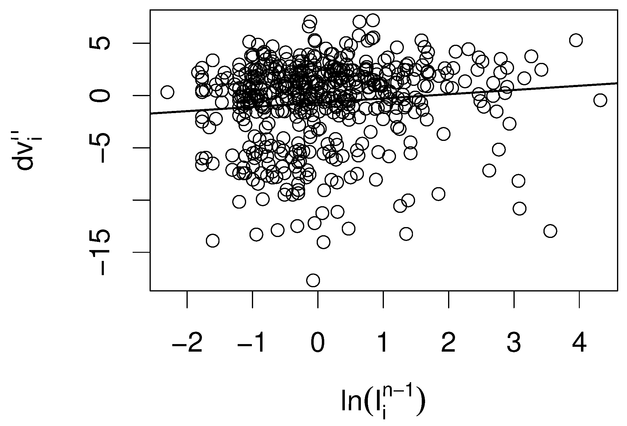
While it is intuitive that vaccination helps not only individuals but also the protection of the population, it is less clear if parents respond to local measles outbreaks such that vaccination coverage increases. Moreover, we test for a delay in the response of the parents to an outbreak. Thus, we consider the difference in the vaccination coverage of next year and this year, and test by a linear model for an effect of the incidence of this year, last year, and the year before last year.

We find that only the incidence with a delay of one year has a significant ($p=0.015$) positive point estimate (

Table 3. $v_i^n$ denotes the vaccination coverage, and $I_i^n$ the incidence (per 100,000). We explain $d{v}_i^n=v_i^{n+1}-v_i^n|I_i^n>0$ by a linear model with the factor $ln\left(I_i^{n-\tau }\right)$, where $\tau$ is the delay ($\tau =0$, $\tau =1$, and $\tau =2$ is tested). “Coeff.”: coefficient estimate. p-value: significance level.

	Coeff. ln(Incidence)	p-Value
No delay	−0.1	0.51
1 year delay	0.4	0.015
2 years delay	−0.3	0.08

and Figure 3), while the other two years have negative point estimates.

3. Mechanistic Model for Measles Dynamics

The findings of the statistical data analysis showed that vaccination reduces incidence. Furthermore, a measles outbreak does induce a higher vaccination rate, but with a certain delay. In order to cover both effects, we combine a Kermack–McKendrick-type model and an opinion-dynamics model. The Kermack–McKendrick model augmented by vaccination is standard to address the time course of the infection [31,32]. In our model, the vaccination rate is under control of an opinion dynamics model, which bears some similarity with the zealot model [33,34,35,36]. The public opinion is influenced by measles outbreaks, but only with a certain delay.

We start off with a stochastic opinion model. At time t, a population of finite size $N\in \mathbb{N}$ is made up of $X_t$ pro-vaccination individuals and $N-X_t$ individuals holding an anti-vaccination opinion. We assume this composition is at a dynamic equilibrium in the absence of infections, with an equal rate for each person to reconsider her opinion. In absence of the infection, there are fixed rates from pro- to anti-vaccination and opposite, such that we will observe an invariant distribution. However, parents might respond to the presence of the infection. The rate from anti-vaxxers to pro-vaccination is assumed to depend linearly on the prevalence. If we fix the prevalence I, the rates from pro- to anti-vaccination and vice versa become

$$\begin{array}{ccc}\hfill X_t& \to & X_t+1\mathrm{at} \mathrm{rate}(N-X_t)(b+cI(t-\tau )/N)\hfill \\ \hfill X_t& \to & X_t-1\mathrm{at} \mathrm{rate} X_{t}a\hfill \end{array}$$

where $a,b,c>0$ are parameters of the opinion model, and $\tau$ is the delay in the response of the opinion dynamics on the prevalence.

If $x\left(t\right)=E(X_t/N)$, we easily find the ODE

$$\frac{d}{dt}x\left(t\right)=(1-x\left(t\right))(b+cI(t-\tau )/N)-ax\left(t\right)$$

with only one, globally stable, stationary state $\widehat{x}$,

$$\widehat{x}=\frac{b+cI(t-\tau )/N}{a+b+cI/N}.$$

That is, $E(X_t/N)\to \widehat{x}$ in the long run in case of constant I.

We now formulate the infection dynamics, first without opinion dynamics. We have a classical SIR model with population dynamics and vaccination, where a fraction $\rho$ of the newborn is vaccinated (no vaccination of older children). This is, for sure, a strong simplification, but this simple model is sufficient to understand the effects we aim at. We find

$$\begin{array}{ccc}\hfill S^{\prime }& =& (1-\rho )N\mu -\beta \frac{SI}{N}-\mu S\hfill \\ \hfill I^{\prime }& =& \beta \frac{SI}{N}-\gamma I-\mu I\hfill \\ \hfill R^{\prime }& =& \rho N\mu +\gamma I-\mu R.\hfill \end{array}$$

As usual, N is the total population, $\mu$ the recruiting rate, $\beta$ the proportionality constant of the standard incidence term, and $\gamma$ the recovery rate.

To combine the opinion and the infection model, we implicitly assume that the opinion formation model is in equilibrium (which does mean we have a time scale separation, $a,b,c\gg 0$). We then assume that the expected fraction of the pro-vaccination population determines the fraction of vaccinated kids,

$$\rho =F(I(t-\tau )/N),F\left(x\right)=\frac{b+cx}{a+b+cx}.$$

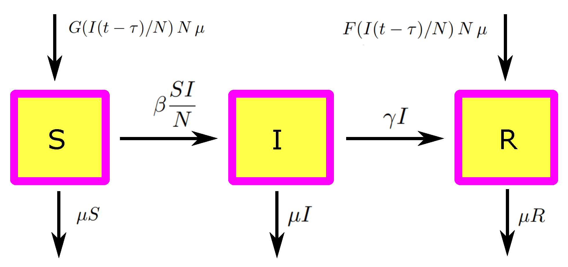
Therewith, we obtain the complete model depicted in Figure 4 (which is focused on the basic mechanisms, and can easily extended to become more realistic).

$$\begin{array}{ccc}\hfill S^{\prime }& =& G\left(I(t-\tau )\right)/N)N\mu -\beta \frac{SI}{N}-\mu S\hfill \\ \hfill I^{\prime }& =& \beta \frac{SI}{N}-\gamma I-\mu I\hfill \\ \hfill R^{\prime }& =& F\left(I\right(t-\tau )/N)N\mu +\gamma I-\mu R\hfill \\ \hfill F\left(x\right)& =& \frac{b+cx}{a+b+cx},G\left(x\right)=1-F\left(x\right)=\frac{a}{a+b+cx}\hfill \end{array}$$

As the equations for S and I are independent of R, we can reduce the system, and consider only

$$\begin{array}{ccc}\hfill S^{\prime }& =& G(I(t-\tau )/N)N\mu -\beta \frac{SI}{N}-\mu S\hfill \end{array}$$

(1)

$$\begin{array}{ccc}\hfill I^{\prime }& =& \beta \frac{SI}{N}-\gamma I-\mu I\hfill \end{array}$$

(2)

$$\begin{array}{ccc}\hfill G\left(x\right)& =& \frac{a}{a+b+cx}.\hfill \end{array}$$

(3)

3.1. Analysis

We first identify stationary states; particularly, we aim at the usual dichotomy, that there is only a disease-free equilibrium (DFE) if the effective reproduction number $R_{eff}$, which is the reproduction number in the presence of vaccination, is below one and that there is additionally a stationary endemic state (a stationary state with non-trivial I component) in case of $R_{eff}>1$.

Proposition 1.

The DFE is provided by $(S_0,I_0)=(G\left(0\right)N,0)$. The effective reproduction number in presence of vaccination is provided by

$$R_{eff}=\frac{\beta G\left(0\right)}{\mu +\gamma }.$$

Proof. 

In the DFE, we have $I=0$, and hence $I^{\prime }=0$ is satisfied. From $S^{\prime }=0$, we obtain $S=S_0=G\left(0\right)N$. Now, we linearize the equation for $I^{\prime }$ at $(S,I)=(S_0,0)$ and obtain

$$I^{\prime }=\beta \frac{S_0}{N}I-\gamma I-\mu I=(\beta G\left(0\right)-\gamma -\mu )I.$$

Therewith, we define $R_{eff}={\int }_0^{\infty }\beta G\left(0\right)e^{-(\mu +\gamma )a}da=\beta G\left(0\right)/(\mu +\gamma )$. □

Proposition 2.

If $R_{eff}>1$, there is a unique endemic equilibrium $(S^{*},I^{*})$, which satisfies

$$\begin{array}{c}\hfill S^{*}=\frac{\gamma +\mu }{\beta }N,G(I^{*}/N)=\frac{\mu +\gamma }{\mu }{I}^{*}/N+\frac{\gamma +\mu }{\beta }.\end{array}$$

(4)

Proof. 

We aim at an equilibrium $(S^{*},I^{*})$ with $I^{*}>0$: From $I^{\prime }=0$ and $I>0$, we obtain

$$\beta \frac{S^{*}}{N}-\gamma -\mu =0\Rightarrow S^{*}=\frac{\gamma +\mu }{\beta }N.$$

We plug this result into $S^{\prime }=0$ and find $0=G(I^{*}/N)N\mu -(\mu +\gamma )I^{*}-\mu \frac{\gamma +\mu }{\beta }N$; that is, with $i^{*}=I^{*}/N\in [0,1]$, we find the condition

$$G\left(i^{*}\right)=\frac{\mu +\gamma }{\mu }{i}^{*}+\frac{\gamma +\mu }{\beta }.$$

Note that $G^{\prime }<0$ and the r.h.s. of the equation is increasing in $i^{*}$. There is, hence, at most one solution.

As $R_{eff}>1$, we know $G\left(0\right)\beta >\mu +\gamma$, and hence

$$G\left(i^{*}\right){|}_{i^{*}=0}>\left(\frac{(\mu +\gamma )}{\mu }{i}^{*}+\frac{\gamma +\mu }{\beta }\right){|}_{i^{*}=0}.$$

Furthermore,

$$G\left(i^{*}\right){|}_{i^{*}=1}\le 1<1+\frac{\gamma }{\mu }<\left(\frac{\mu +\gamma }{\mu }{i}^{*}+\frac{\gamma +\mu }{\beta }\right){|}_{i^{*}=1}.$$

Thus, we have a unique solution that establishes the proposition. □

We now turn to the local stability analysis. For the DFE, we find the usual result: it is (globally) stable if $R_{eff}<1$, and unstable for $R_{eff}>1$.

Proposition 3.

If $R_{eff}<1$, the DFE is globally (in the positive quadrant) stable.

Proof. 

Step 1: First of all, due to the definition of $G\left(x\right)$ in (3), we have $G\left(0\right)\ge G\left(I\right(t-\tau )/N)$, and hence

$$S^{\prime }\le G\left(0\right)N\mu -\mu S$$

such that

$$\underset{t\to \infty }{lim\; sup}S\left(t\right)\le G\left(0\right)N.$$

If $\epsilon >0$, we have hence that any trajectory $(S,I)\in {\mathbb{R}}_{+}^2$ will after finite time enter the the strip

$$\Omega =\left\{\right(S,I\left)\right|0\le S\le G\left(0\right)N+\epsilon N\}.$$

Step 2: We choose $\epsilon$ small enough, such that

$$R_{eff}+\beta \frac{\epsilon }{\mu +\gamma }=\beta \frac{G\left(0\right)+\epsilon }{\mu +\gamma }<1.$$

This is possible as $R_{eff}<1$. We now use $L(S,I)=I$ as a Lyapunov function in $\Omega$,

$$\frac{d}{dt}L(S,I)=I^{\prime }\left(t\right)=\left(\beta \frac{S}{N}-\mu -\gamma \right)\hspace{0.17em}I\le (\mu +\gamma )\left(\beta \frac{G\left(0\right)+\epsilon }{\mu -\gamma }-1\right)\hspace{0.17em}I\le 0$$

where $\frac{d}{dt}L(S,I)=0$ iff $I=0$. Hence, $I\left(t\right)\to 0$. The principle of Lassale now tells us that the $\omega$ limit set of $(S,I)$ is contained in the largest invariant set of $I=0$, which is $\{S=S_0\}$. □

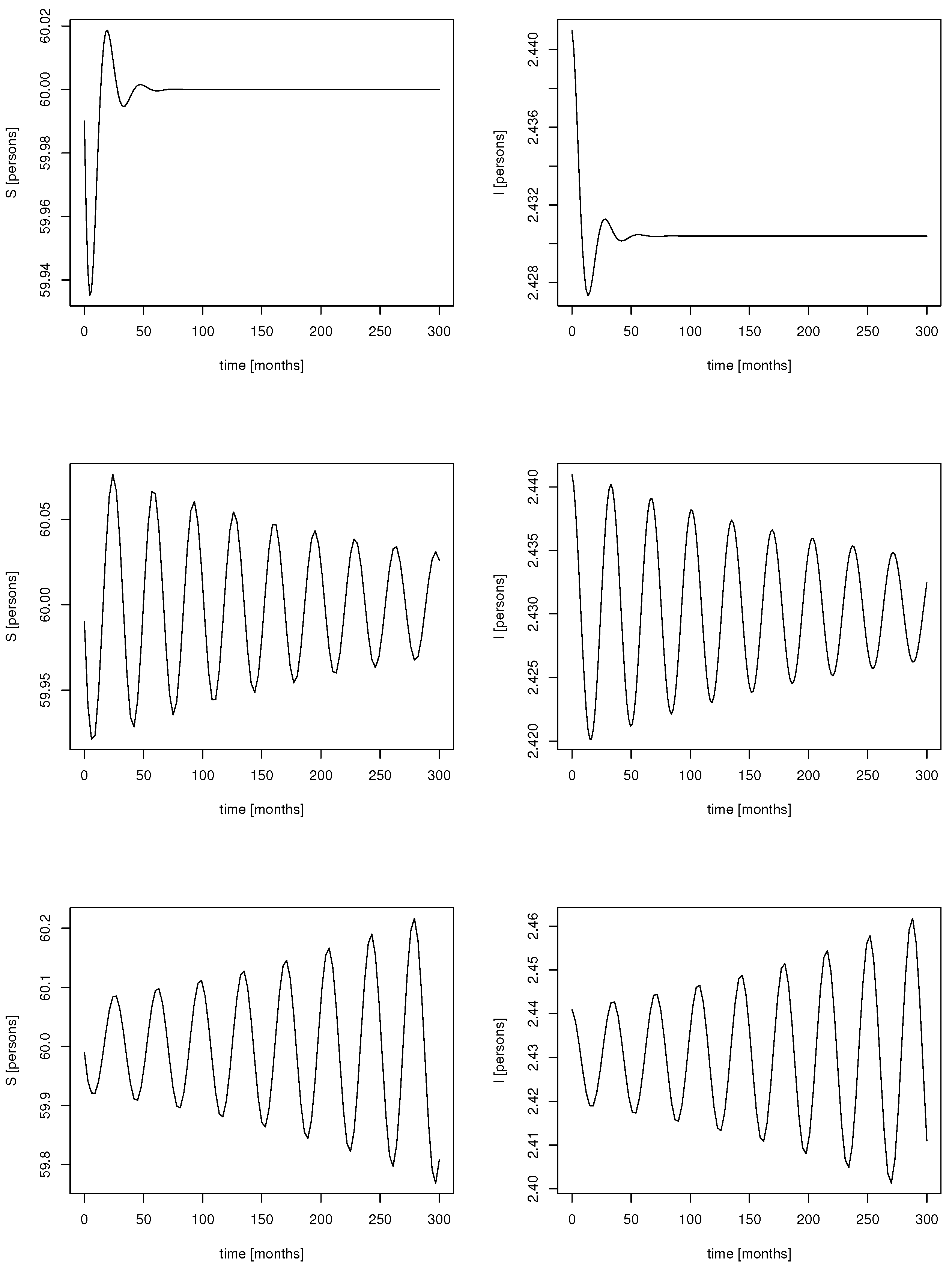
We move to the stability behavior of the endemic equilibrium. As a delay is involved in the dynamics, the endemic equilibrium might lose (linear) stability via a Hopf bifurcation. Indeed, simulations for different delays indicate that sustained oscillations appear if the delay crosses a certain threshold (Figure 5).

Proposition 4.

Let $i^{*}=I^{*}/N$ and $u^{*}=\frac{{(\beta i^{*}+\mu )}^2}{2\beta i^{*}\left|G^{\prime }\left(i^{*}\right)\right|\mu }$. There is ${\tau }_0>0$, such that we have a Hopf point at $\tau ={\tau }_0$, if and only if in case of $u^{*}<1$

$$G^{\prime }{\left(\tilde{i}\right)}^2\ge \frac{{(\beta i^{*}+\mu )}^2[\beta i^{*}(\mu /2+\gamma )-\frac{1}{4}{(\beta i^{*}-\mu )}^2]}{{\left(\beta i^{*}\mu \right)}^2}=:G_{crit}^2.$$

respectively in case of $u^{*}\ge 1$

$$\left|G^{\prime }\left(i^{*}\right)\right|\ge \left(1+\frac{\gamma }{\mu }\right).$$

The endemic equilibrium is locally asymptotically stable for $\tau \in [0,{\tau }_0)$.

The proof, which follows the standard arguments [32] but is slightly technical, can be found in Appendix A. For a Hopf bifurcation to happen, additional non-degeneracy conditions are necessary [37], which we do not check. Instead, we indicate that we indeed find oscillations in numerical simulations (see Figure 5).

Note that, for $G^{\prime }\left(i^{*}\right)=0$ (or sufficiently small), no Hopf point appears, and the endemic solution is for any delay locally asymptotically stable. The response of the population to the incidence needs to be strong enough ($|G^{\prime }\left(i^{*}\right)|$ sufficiently large) to trigger oscillations.

3.2. Realistic Parameter Range

We find that oscillations are possible if the delay is sufficiently large. However, the question arises if these oscillations, driven by the delay we identified in the data, are something to expect. Here, time scales are crucial. We identify parameters accordingly.

First of all, the system is homogeneous of degree 1; that is, for $s\left(t\right)=S\left(t\right)/N$, $i\left(t\right)=I\left(t\right)/N$, and $r\left(t\right)=R\left(t\right)/N$, we again find a proper ODE,

$$\begin{array}{ccc}\hfill s^{\prime }& =& G\left(i\right(t-\tau \left)\right)\mu -\beta si-\mu s\hfill \\ \hfill i^{\prime }& =& \beta si-\gamma i-\mu i\hfill \\ \hfill r^{\prime }& =& F\left(i\right(t-\tau \left)\right)\mu +\gamma i-\mu r\hfill \\ \hfill F\left(x\right)& =& \frac{b+cx}{a+b+cx},G\left(x\right)=1-F\left(x\right)=\frac{a}{a+b+cx}=\frac{1}{1+(b/a)+(c/a)x}.\hfill \end{array}$$

Therefore, we do not need to specify N. As we are only interested in children under 5 years old, say, we take $\mu =1/5$ (with years as the basic time unit). The time a person is sick is about 9 days, which gives us $\gamma =365/9\approx 39.5$. Furthermore, the basic reproduction number $R_0=\beta /(\mu +\gamma )\approx 10$, and thus we choose $\beta \approx 400$. The only parameters that remain to be determined are the opinion dynamics parameters. We only require two lumped parameters here: $\tilde{b}:=b/a$ and $\tilde{c}:=c/a$. We find that $\tilde{b}/(1+\tilde{b})=F\left(0\right)$ denotes the fraction of vaccinated children in absence of a previous measles outbreak. Unlike the epidemic parameters, we do not have standard values for the opinion formation part of the model; therefore, we consider two different scenarios (

Table 4. Values for the deterministic model that are in a reasonable range. Recall that $F\left(0\right)$ denotes the fraction of vaccinated newborns in absence of the infection (baseline vaccination). For a discussion of the parameter choice, see text.

Meaning	Variable	Scenario 1	Scenario 2
removal rate	$\mu$	0.2 yr−1	0.2 yr−1
recovery rate	$\gamma$	39.5 yr−1	39.5 yr−1
contact rate	$\beta$	400 yr−1	400 yr−1
delay	see text	1 year	see text
opinion model, basic parameter	$\tilde{b}=b/a$	4 (⇒F(0) = 0.8)	0.1 (⇒F(0) = 0.1)
opinion model, response to an outbreak	$\tilde{c}=c/a$	100	100

). For scenario 1, we take the typical vaccination coverage of Germany as a basis, s.t. $\tilde{b}/(1+\tilde{b})\approx 0.5,\dots ,0.9$. We choose $\tilde{b}=4$, corresponding to $F\left(0\right)=0.8$. In scenario 2, we consider a much lower average vaccination coverage, where only 10% of the children are vaccinated, such that $\tilde{b}=0.1$. Last, we need to specify how strong the response to a local outbreak might be. We assume the rather optimistic value $\tilde{c}=100$ for both scenarios; we need to take into account that the prevalence, the fraction of infected children at a given time point, will be tiny, such that $\tilde{c}$ needs to be large in order to allow the prevalence to have a distinct influence.

For scenario 1, we find $R_{eff}=G\left(0\right)\beta /(\gamma +\mu )\approx 2>1$, such that we have a positive endemic equilibrium. Herein,

$$s^{*}=\frac{S^{*}}{N}=\frac{\gamma +\mu }{\beta }\approx 0.1$$

while the prevalence in equilibrium $i^{*}=I^{*}/N$ is provided by the fixed point equation stated in (4). Numerical analysis yields

$$i^{*}=0.0005.$$

Therewith, we numerically obtain $u^{*}=0.51$, $G^{\prime }{\left(i^{*}\right)}^2=15.4$, while the corresponding threshold for $G^{\prime }{\left(i^{*}\right)}^2$ stated in Theorem 4 is $G_{crit}^2=792$. A Hopf point is not possible, even in case of a long delay. A much stronger response is required until periodic orbits can appear.

If we turn to scenario 2, we have $R_{eff}=G\left(0\right)\beta /(\gamma +\mu )\approx 10>1$, and, as before,

$$s^{*}=\frac{S^{*}}{N}=\frac{\gamma +\mu }{\beta }\approx 0.1,$$

as the fraction of susceptibles is not affected by the opinion model. We find by numerical analysis

$$i^{*}=0.003,u^{*}=0.08.G^{\prime }{\left(i^{*}\right)}^2=2579.5>1634.1=G_{crit}^2.$$

Therefore, periodic orbits may appear if the delay is sufficiently long. Again, numerical analysis (based on the formula developed in Appendix A) indicates a minimal length for the delay of ${\tau }_0=0.134$ years (ca. $1.5$ months), leading to a period of $T=0.84$ years (ca. 10 months).

In Figure 6, the bifurcation diagram is shown for three levels of the baseline vaccination. Theorem 4 indicates that, only for a baseline vaccination coverage that is sufficiently small, oscillations are possible; we have seen above that, for scenario 1, with 80% baseline vaccination, no oscillation can be induced. Figure 6 indicates that, for 50% vaccination and below, we easily find sustained oscillation, provided that the social response appears with a certain strength. If that is given, even a short or moderate delay of a few weeks (2–4 weeks) leads to sustained oscillations with a period of about one year. The period of these oscillations does not depend crucially on the delay or the strength of the response.

4. Discussion

In this study, we discuss a possible social response of the population to the presence of measles. In the first part of the study, we focused on the statistical analysis of vaccination data and measles prevalence for 345 districts in Germany, for the years 2008–2012. It is not surprising that a higher vaccination coverage indicates a lower size of a local outbreak. What might be surprising is that the probability of an outbreak is unrelated to the vaccination coverage. Here, we note that the overall vaccination coverage in Germany at this time is sufficiently high to break local transmission chains [38]. The central cause for the appearance of local outbreaks is non-local infectious contacts. The frequency of these contacts is approximately independent of the vaccination coverage but depends on the global force of infection.

The central finding of the present study is that an increase in vaccination converges on a local outbreak. The only parallel finding known by the authors is the study by Philipson [7] in 1996, who found strong evidence in data for the US between 1984 and 1990 that children are vaccinated at younger ages if the measles incidence is high. As the data we use are noisy, we are only able to identify the effects of local outbreaks due to the fact that we have localized data, which means on the one hand that parents have a chance to be aware of these outbreaks (the outbreak did take place, most likely, in the vicinity), and we have a large sample. However, we do not test for spatial interaction effects: outbreaks in neighboring districts might also have some effect. Most interesting is the delay in the response. As vaccination usually takes place between 11 and 14 months, it is most likely that the mother was still pregnant with the child during the outbreak. This finding may indicate that particularly pregnant women are susceptible to information about infectious diseases, which should be investigated in more focused studies.

The statistical analysis reveals another aspect, namely that significant spatial differences in vaccination coverage exist. Possible explanations are the different histories of former West and East Germany [38], which still influence the population. Also, opinion dynamics might contribute, as investigated in [22].

In the second part of the paper, we turn to the investigation of a mechanistic model, in the same spirit as Philipson [7] (where his model is mainly concerned with the effects of the price of the vaccine). In the present study, we particularly focus on the delay in opinion dynamics. The analysis shows that this delay is able to trigger periodic orbits, and a consistency check with realistic parameter values indicates that the periodic orbits might be reasonable if the vaccination coverage is rather low and the response is rather strong. However, because measles is influenced by periodically changing contact patterns [39] (school vacations or rainy seasons in Africa), it is likely that the periodicity triggered by the social response is overshadowed by these periodic background patterns. The interaction between the nonlinear intrinsic social feedback and the extrinsically caused periodicity in the contact rate might induce bifurcations, which lead to complex behavior. In case of other infections, the importance of social response was presumably more distinct, although it is perhaps more difficult to clearly identify in data. During the COVID-19 pandemic, part of the population initially adhered strictly to the rules of social distancing but eventually became tired of these rules and behaved carelessly again [40,41]. One might speculate that the incidence first went down to eventually rise again. The waves we have observed can be mostly attributed to new virus variants, but the social response might also have contributed.

We learn from this study that social responses in the dynamics of infectious diseases cannot be neglected. From a modeling perspective, it is unclear how to account for these social mechanisms. The scientific community agrees on Kermack–McKendrick-like models, which are powerful tools for the analysis and prediction of the time course of infectious diseases but do not incorporate social feedback. However, if mathematical epidemiology aims to be a reliable tool for public health authorities, a better understanding of the behavioral changes and social responses of the population to the presence of infections is necessary. We have many rather theoretical attempts speculating about the behavioral effects based on game theory [9,10,11] or social learning [13,14]. We only have very few examples that aim to find these effects in data: for example, the study of Philipson [7] for measles, or that of Barzon et al. [1] for COVID-19. We need more studies that tightly integrate statistical and mechanistic models to reach a clear agreement on how to model this effect, how important such effects are in situations of practical relevance, which consequences to expect, and how to estimate the parameters of these models in a reliable way.