Article

Computationally Efficient Poisson Time-Varying Autoregressive Models through Bayesian Lattice Filters

1
Amazon.com, Inc., New York, NY 10001, USA
2
Department of Statistics, University of Missouri, Columbia, MO 65211-6100, USA
3
Office of the Associate Director for Research and Methodology, Research and Methodology Directorate, U.S. Census Bureau, Washington, DC 20233-9100, USA
4
School of Agriculture and Food Sciences, The University of Queensland, St Lucia, QLD 4072, Australia
5
School of Mathematics and Physics, The University of Queensland, St Lucia, QLD 4072, Australia
*
Author to whom correspondence should be addressed.
Stats 2023, 6(4), 1037-1052; https://doi.org/10.3390/stats6040065
Submission received: 16 August 2023 / Revised: 26 September 2023 / Accepted: 4 October 2023 / Published: 9 October 2023

Abstract

:
Estimation of time-varying autoregressive models for count-valued time series can be computationally challenging. In this direction, we propose a time-varying Poisson autoregressive (TV-Pois-AR) model that accounts for the changing intensity of the Poisson process. Our approach can capture the latent dynamics of the time series and therefore make superior forecasts. To speed up the estimation of the TV-AR process, our approach uses the Bayesian Lattice Filter. In addition, the No-U-Turn Sampler (NUTS) is used, instead of a random walk Metropolis–Hastings algorithm, to sample intensity-related parameters without a closed-form full conditional distribution. The effectiveness of our approach is evaluated through model-based and empirical simulation studies. Finally, we demonstrate the utility of the proposed model through an example of COVID-19 spread in New York State and an example of US COVID-19 hospitalization data.

1. Introduction

Modeling count time series is essential in many applications such as pandemic incidences, insurance claims, and integer financial data such as transactions. Different types of count time series models have been broadly developed within the two classes of observation-driven and parameter-driven models [1,2], where in an observation-driven model, current parameters are deterministic functions of lagged dependent variables as well as contemporaneous and lagged exogenous variables, while in parameter-driven models, parameters vary over time as dynamic processes with idiosyncratic innovations. The observation-driven models include the integer-valued generalized autoregressive conditional heteroskedasticity (INGARCH) model [3,4], integer-valued autoregressive model, also called Poisson autoregressive model [5], generalized linear autoregressive moving average (GLARMA) model [6,7], and Poisson AR model [8], among others (see [9,10] for a comprehensive overview). The parameter-driven models include the Poisson state space model [11], Poisson exponentially weighted moving average (PEWMA) model [12], and dynamic count mixture model [13], among others. Some of this research proceeds under a Bayesian framework [13,14,15].
For nonstationary count time series with changing trends, e.g., daily new COVID cases data, the stationary methods [3,4,8,12] may not capture local trends or give good multi-step-ahead forecasts. The motivation for our study is to propose an efficient method by which to capture the time-varying pattern of the means for such nonstationary count time series and therefore make better forecasts than traditional methods. To capture the evolutionary properties, a parameter-driven (process-driven) model with a time-varying coefficient latent process is a good choice. Moreover, a latent process with appropriately modeled innovations can address the potential over-dispersion issue, which is common in count time series modeling.
We propose a time-varying Poisson autoregressive (TV-Pois-AR) model for nonstationary count time series and utilize the efficiency of the Bayesian lattice filter (BLF, [16]) and the no-U-turn sampler (NUTS, [17,18]) together to estimate the model parameters. We use a time-varying autoregressive (TV-AR) latent process to model the nonstationary intensity of the Poisson process. This flexible model can capture the latent dynamics of the time series and therefore make superior forecasts. The estimation of such a TV-AR process is greatly sped up by using BLF. Moreover, NUTS is used to sample the intensity-related parameters which have no analytical forms of full conditional distributions. NUTS is an extension to the Hamilton Monte Carlo (HMC, [19,20,21]) algorithm via automatic tuning of the step size and the number of steps. The use of the HMC method inside the Gibbs sampling was investigated in [22]. According to their paper, as a self-tuned extension to HMC, NUTS should work well as a univariate sampler inside the Gibbs sampling. Benefiting from the joint use of the Bayesian lattice filter and no-U-turn sampler, the estimation of the TV-Pois-AR model is efficient and fast, especially for higher model orders or longer length time series. In short, our main contribution is computational in that we develop a methodology for the efficient estimation of Poisson time-varying autoregressive models.
The rest of the paper is organized as follows. In Section 2, we formulate the proposed Bayesian time-varying coefficient Poisson model. In Section 3, we present a simulation study that illustrates the small sample properties of the proposed Bayesian estimators. In Section 4, our proposed model is demonstrated through an example of COVID-19 spread in New York State and an example of US COVID-19 hospitalization data. In Section 5, we summarize the proposed method and discuss possible future research directions. In the Appendices, the detailed algorithms are introduced.

2. Methodology

2.1. TV-Pois-AR(P) Model

For a univariate count-valued series,  z t t = 1 , , T , we propose a TV-Pois-AR model of order P (TV-Pois-AR(P)) defined as
z t | X t ψ , y t Pois ( exp ( X t ψ + y t ) ) , y t = j = 1 P a j , t y t j + ξ t , ξ t N ( 0 , σ t 2 ) ,
where exp ( · )  stands for the exponential function,  X t  is  1 × K  vector of covariates,  ψ  is a  K × 1  vector of coefficients, and  y t  is the autoregressive component of the logarithm of the Poisson intensity, which follows a TV-AR process. Depending on the specific application case,  X t ψ  can be a constant term  μ  or removed from the model. Throughout the context, we use a constant term  μ  and do not consider any covariate. We define  a j , t  and  σ t 2  to be the time-varying AR coefficients of TV-AR(P) associated with time lag j at time t and the innovation variance at time t, respectively. The innovations,  ξ t , are defined to be independent Gaussian errors.

2.2. Bayesian Lattice Filter for the TV-AR Process

Under the Bayesian framework, a major part of the model inference is the estimation of parameters in the latent TV-AR process of  y t , the posterior distributions of which are not conjugate. Using Monte Carlo methods to generate converged sample chains for the time-varying parameters constitutes a large computational burden. BLF provides an efficient way to directly obtain the posterior means of these time-varying parameters. Using the posterior means as MC samples greatly accelerates the convergence of sample chains. According to the Durbin–Levinson algorithm, there exists a unique correspondence between the partial autocorrelation (PARCOR) coefficients and the AR coefficients [16,23,24]. This lattice structure provides an efficient way to estimate the PARCOR coefficients, which are associated wit AR models (see [25] and the Supplemental materials [16]). The efficient estimation of this TV-AR process can be conducted through the following P-stage lattice filter. We denote  f t ( P )  and  b t ( P )  to be the prediction error at time t for the forward and backward TV-AR(P) models, respectively, where
f t ( P ) = y t j = 1 P a j , t ( P ) y t j , b t ( P ) = y t j = 1 P d j , t ( P ) y t + j ,
and  a j , t ( P )  and  d j , t ( P )  are the forward and backward autoregressive coefficients of the corresponding TV-AR(P) models. Then, in the jth stage of the lattice filter for  j = 1 , , P , the forward and the backward coefficients and the forward and backward prediction errors have the following relationship:
f t ( j ) = f t ( j 1 ) α j , t ( j ) b t j ( j 1 ) , b t ( j ) = b t ( j 1 ) β j , t ( j ) f t + j ( j 1 ) ,
where  α j , t ( j )  and  β j , t ( j )  are the lag j forward and backward PARCOR coefficients at time t, respectively. The initial condition,  f t ( 0 ) = b t ( 0 ) = y t , can be obtained from the definition in (3). This implies that the samples of  y t  are plugged in as the initial values of  f t ( 0 )  and  b t ( 0 )  in the Gibbs sampling. At the jth stage of the lattice structure, we fit time-varying AR(1) models to estimate  α j , t ( j )  and  β j , t ( j ) . The corresponding forward and backward autoregressive coefficients at time t a j , t ( j )  and  d j , t ( j )  can be obtained according to the following equations:
a i , t ( j ) = a i , t ( j 1 ) a j , t ( j ) d j i , t ( j 1 ) , d i , t ( j ) = d i , t ( j 1 ) d j , t ( j ) a j i , t ( j 1 ) ,
with  i = 1 , , j 1 a j , t ( j ) = α j , t ( j )  and  d j , t ( j ) = β j , t ( j ) . Finally, the distribution of  a j , t ( P )  and  ξ t  for  j = 1 , , P  are obtained. These distributions are used as conditional distributions of  a j , t  and  ξ t  in the Gibbs sampling.

2.3. Model Specification and Bayesian Inference

We assume that each coefficient in  β  has a conjugate normal prior distribution, i.e.,  β k i . i . d . N ( μ 0 , τ 0 2 ) , and the initial state of the latent variable  y 0  follows a normal distribution, s.t.,  y 0 N ( m 0 , s 0 2 ) . In Gibbs sampling,  μ  is sampled efficiently by NUTS, and this speeds up the mixing of the sample chains. Compared to the Metropolis–Hastings algorithm, which uses a Gaussian random walk as proposal distribution, NUTS generates samples converging to the target distribution. The target distribution of  y t , for  t = 1 , , T , is its conditional distribution with the density function
p ( y t | z t , y t , θ ) = p ( z t | μ , y t ) p ( y t | y t , θ ) p ( z t | μ + y t ) p ( y t | y t 1 , θ ) p ( y t + 1 | y t , θ ) ,
where  y t = ( y t , , y t P + 1 ) θ  denotes  a j , t , and  σ t 2  for all t and  y t  denotes  y i  for all i but t. According to the previous assumptions, the conditional distributions of  z t  is Poisson and the conditional distributions of  y t  and  y t + 1  are Gaussian. Having the target distribution, NUTS can adaptively draw samples of  y t  conditional on all other variables for all t.
To use the BLF to derive the conditional distributions of the parameters in the latent autoregressive process of  y t , we define the distribution of its coefficients  a j , t ( P )  by defining the distributions of the forward and backward PARCOR coefficients in (3). To give time-varying structures to the forward and backward PARCOR coefficients, we consider random walks for the PARCOR coefficients. The PARCOR coefficients are modeled as
α j , t ( j ) = α j , t 1 ( j ) + ϵ α , j , t , ϵ α , j , t N ( 0 , ω α , j , t ) , β j , t ( j ) = β j , t 1 ( j ) + ϵ β , j , t , ϵ β , j , t N ( 0 , ω β , j , t ) ,
where  ω α , j , t  and  ω β , j , t  are time dependent evolution variance. These evolution variances are defined via the standard discount method in terms of the discount factors  γ f , j  and  γ b , j  within the range  ( 0 , 1 ) , respectively (see Appendix A, Appendix B, Appendix C and Appendix D and [26] for details). The discount factor  γ  controls the smoothness of PARCOR coefficients. Here, we assume  γ f , j = γ b , j = γ j  at each stage j. Similarly, the innovation variances are assumed to follow multiplicative random walks and modeled as
σ f , j , t 2 = σ f , j , t 1 2 ( δ f , j / η f , j , t ) , η f , j , t β ( g f , j , t , h f , j , t ) , σ b , j , t 2 = σ b , j , t 1 2 ( δ b , j / η b , j , t ) , η b , j , t β ( g b , j , t , h f , j , t ) ,
where  δ f , j  and  δ b , j  are also discount factors in the range (0, 1), and the multiplicative innovations,  η f , j , t  and  η b , j , t , follow beta distributions with hyperparameters ( g f , j , t , h f , j , t ) and ( g b , j , t , h f , j , t ) (see Appendix A, Appendix B, Appendix C and Appendix D and [26] for details). The smoothness of innovation variance is controlled by both  γ  and  δ . Similar to the PARCOR coefficients, we assume  δ f , j = δ b , j = δ j  at each stage. Note that  ϵ α , j , t ϵ β , j , t η f , j , t , and  η b , j , t  are mutually independent and are also independent of any other variables in the model. The discount factors  γ  and  δ  are selected adaptively through a grid-search based on the likelihood (see the Appendix A, Appendix B, Appendix C and Appendix D for details) in each iteration of MCMC.
We specify conjugate initial priors for the forward and backward PARCOR coefficients, so that
p ( α j , 0 | D f , j , 0 , σ f , j , 0 ) N ( μ f , j , 0 , C f , j , 0 ) , p ( β j , 0 | D b , j , 0 , σ b , j , 0 ) N ( μ b , j , 0 , C b , j , 0 ) ,
where  p = 1 , , P D f , j , 0 D b , j , 0  denotes the information available at the initial time  t = 0 , and  μ f , j , 0  and  C f , j , 0  are the mean and the variance of the normal prior distribution. We also specify conjugate initial priors for the forward and backward innovation variance, so that
p ( σ f , j , 0 2 | D f , j , 0 ) G ( ν f , j , 0 / 2 , κ f , j , 0 / 2 ) , p ( σ b , j , 0 2 | D b , j , 0 ) G ( ν b , j , 0 / 2 , κ b , j , 0 / 2 ) ,
where  G ( · , · )  is the gamma distribution, and  ν f , j , 0 / 2  and  κ f , j , 0 / 2  are the shape and rate parameters for the gamma prior distribution. Usually, we treat these starting values as constants over all stages. In order to reduce the effect of the prior distribution, we choose  μ f , j , 0 / 2  and  C f , j , 0  to be zero and one, respectively, and fixed  ν f , j , 0 = 1  and set  κ f , j , 0  equal to  ν f , j , 0  divided by the sample variance of the initial part of each series according to the formula for the expectation of the gamma distribution. The conjugate initial priors for  β j , 0  and  σ b , j , 0 2  are specified in manner analogous to those of  α j , 0  and  σ f , j , 0 2 . A sensitivity analysis was conducted and showed that the simulation studies in Section 3 and the case studies in Section 4 are not sensitive to the choice of the priors and the hyperparameters. In such prior settings, we can use the DLM sequential filtering and smoothing algorithms [26] to derive the joint conditional posterior distributions of the forward and backward PARCOR coefficients and innovation variances in (3). Conditional on the other variables and the data, the full conditional distribution of the latent variable  y t  can easily be obtained individually. To efficiently draw samples from the individual full conditional distribution for the  y t s , we use the NUTS algorithm [17] instead of a traditional random walk Metropolis. The detailed algorithms for the Gibbs sampling, the BLF and the sequential filtering and smoothing are given in Appendix A, Appendix B, and Appendix C.

2.4. Model Selection

In order to determine the model order, we set a maximal order  P m a x  and fit TV-Pois-AR(P) for  P = 1 , , P m a x . The model selection criteria are computed one by one for any specified order. By comparing model selection criteria, we can select the best model order. Since Bayesian inference for the TV-Pois-AR model is conducted through MCMC simulations, we choose the deviance information criterion (DIC) [27,28] and the widely applicable information criterion (WAIC) [29,30].

2.5. Forecasting

Having estimated all parameters, we consider 1-step-ahead forecasts of the TV-Pois-AR(P) model. Then, the 1-step-ahead predictive posterior distribution of the PARCOR coefficients and innovation variance can be obtained according to [26]. The samples of the PARCOR coefficients and innovation variance can be drawn from their predictive distribution. The samples of the 1-step-ahead prediction of the parameters  a T + 1 = ( a 1 , T + 1 , , a P , T + 1 )  can be obtained through the Durbin–Levinson algorithm from the samples of the PARCOR coefficients. After drawing the samples of innovation variance  σ T + 1 2  from its predictive distribution, the samples of  y T + 1  are drawn from its predictive distribution, such that
y T + 1 ( j ) | y 1 : T , a T + 1 ( j ) , σ T + 1 2 ( j ) N ( p = 1 P a p , T + 1 ( j ) y T + 1 p , σ T + 1 2 ( j ) ) , j = 1 , , J .
with the samples of  μ  from its posterior distribution, the samples of the 1-step-ahead forecast are given as
z T + 1 ( j ) | y T + 1 ( j ) , μ ( j ) Pois ( exp ( y T + 1 ( j ) + μ ( j ) ) ) , j = 1 , , J .
We use the posterior median of  z T + 1  obtained through the samples in (5) as the 1-step-ahead forecast. This forecast can be easily extended to h-steps ahead. The details of forecasting up to h-steps ahead can be found in the Appendix A, Appendix B and Appendix C.

3. Simulation Study

In this section, first, we simulate the nonstationary Poisson time series from the exact TV-Pois-AR(P) model to evaluate the parameter estimation of the latent TV-AR process. Second, we generate a nonstationary Poisson time series based on a known time-dependent intensity parameter in order to compare our TV-Pois-AR model with other models. This constitutes an empirical simulation.

3.1. Simulation 1

We simulated 100 time series for each of the lengths  T = 200 , 300 , 400  from the following Poisson TV-AR(6) model, for  t = 1 , , T ,
z t | μ , y t Pois ( exp ( μ + y t ) ) , y t = 6 j = 1 ϕ j , t y t j + ξ t , ξ t N ( 0 , 1 ) ,
where  μ = 3 , which gives a constant mean level to the intensity. The latent process of  y t  is the same time-varying TV-AR(6) process as in [31]. This TV-AR(6) process can be defined as  ϕ t ( B ) y t = ξ t t = 1 , , T , through a characteristic polynomial function  ϕ t ( B ) , with B as the backshift operator (i.e.,  B p y t = y t p ). In this TV-AR(6) process, the characteristic polynomial function is factorized as
ϕ t ( B ) = ( 1 ϕ t , 1 B ) ( 1 ϕ t , 1 * B ) ( 1 ϕ t , 2 B ) ( 1 ϕ t , 2 * B ) ( 1 ϕ t , 3 B ) ( 1 ϕ t , 3 * B ) ,
where the superscript * denotes the complex conjugate of a complex number. Moreover, let  ϕ t , j 1 = A p exp ( 2 π i d t , j )  for  p = 1 , 2 , 3 , where the  d t , j s  are defined by  d t , 1 = 0.05 + ( 0.1 / ( T 1 ) ) t d t , 2 = 0.25 , and  d t , 3 = 0.45 ( 0.1 / ( T 1 ) ) t , and the values of  A 1 A 2 , and  A 3  are equal to  1.1 1.12 , and  1.1 , respectively. Here, we take  T = 200 , 300, and 400 to be of a similar order to our case study in Section 4.1. According to DIC and WAIC,  98 %  of the simulated datasets are identified to follow an order-6 model (TV-Pois-AR). To evaluate the parameter estimation of time-varying parameters, we use the mean squared error (MSE); that is, the average of the squared difference between the estimated parameter value and its true value at each observed time point. Table 1 and Figure 1 and Figure 2 show the MSEs of 6 time-varying autoregressive coefficients, the time-varying innovation variance, the mean level  μ , and the latent variable  y t  over 100 simulated datasets. As expected, when the series length increases, the TV-Pois-AR model gives a more accurate estimation of each parameter.

3.2. Simulation 2—An Empirical Simulation

In this study, we simulated the signals based on the COVID-19 data in New York State (see Section 3.1 for a complete discussion) so that they exhibit similar properties. We generated 100 time series of length  T = 278  from a Poisson process:
z t | λ t Pois ( λ t ) , t = 1 , , T ,
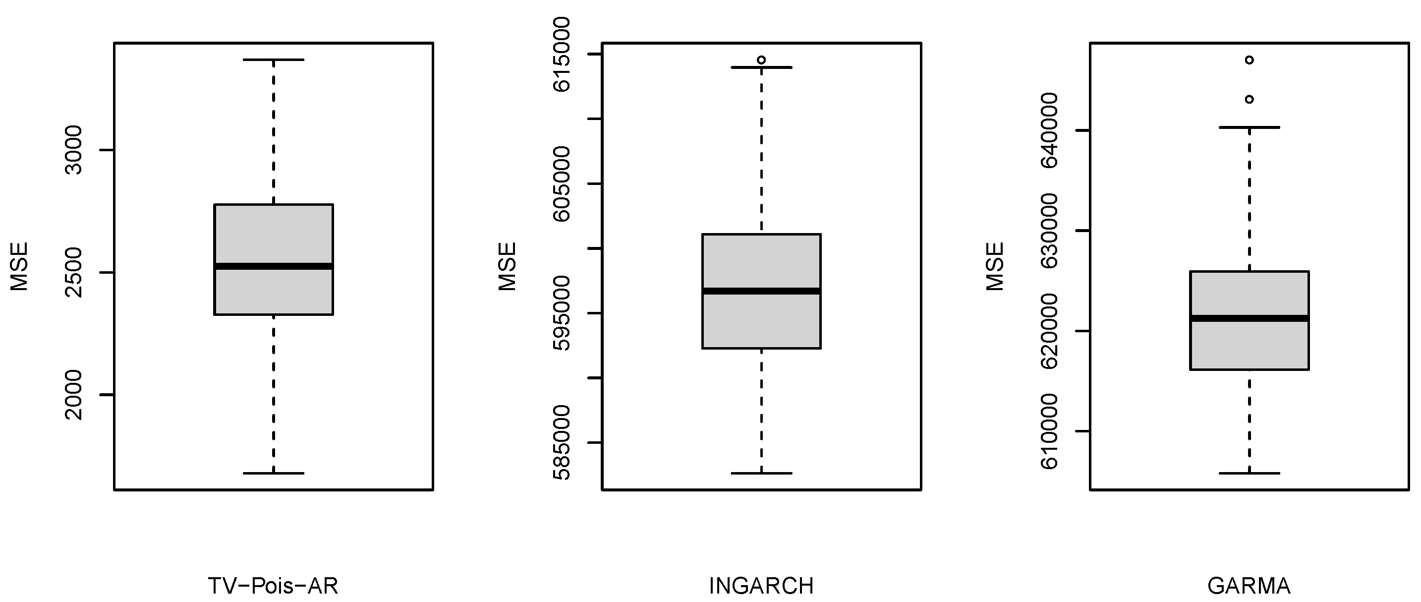
where  λ t  was the 7-day moving average of the estimated intensity of daily new COVID-19 cases in New York State from 3/3/2020 to 12/5/2020. With this type of nonstationary signal, different models are compared by the estimation of the known time-varying intensity parameter  λ t , including the INGARCH and GLARMA model. The INGARCH and GLARMA models are conducted via tsglm from R package tscount. Although these models have different underlying assumptions, they are sometimes used in practices as they can still provide reasonable forecasts. Using the Akaike information criterion (AIC) and the quasi information criterion (QIC) [32], INGARCH(1,0) and GLARMA(1,0) are selected. Both DIC and WAIC indicate that TV-Pois-AR(1) is the best model for these simulated datasets (see details in Section 2.4). To compare the estimation from the frequentist and Bayesian models, the average MSE (AMSE) of the Poisson intensity parameter is computed and shown in Table 2 and Figure 3, where  AMSE = 1 100 T s = 1 100 t = 1 T ( λ t λ ^ t ) 2 . The boxplots in Figure 4 summarize the MSEs of 100 simulated datasets. The estimated intensity figure shows the mean and  90 %  coverage interval by the three models. As shown, TV-Pois-AR makes better forecasts on these simulated datasets. We expect the TV-Pois-AR model to give a better performance than INGARCH and GLARMA on similar pandemic data and other nonstationary count time series that show similar characteristics.

4. Case Studies

To illustrate our proposed methodology, we provide two case studies. The first case study considers COVID-19 case in the New York State; whereas the second case study considers COVID-19 hospitalizations in the U.S. Both case studies are meant to be an illustration of the methodology and thus do not represent a substantive analysis of the COVID-19 pandemic.

4.1. Case Study 1: COVID-19 in New York State

We obtained the 278 daily numbers of confirmed COVID-19 cases in New York State from 3/3/2020 to 12/5/2020 from The COVID Tracking Project (https://covidtracking.com (accessed on 2/7/2021)). We picked New York State data as New York city remained an epicenter in the U.S. for about a month. Our research is motivated by the time-varying nature of the COVID-19 data. Inferences on the trend of the data may give us some insight into the spread of COVID-19 and, possibly, insight into the effect of government interventions.
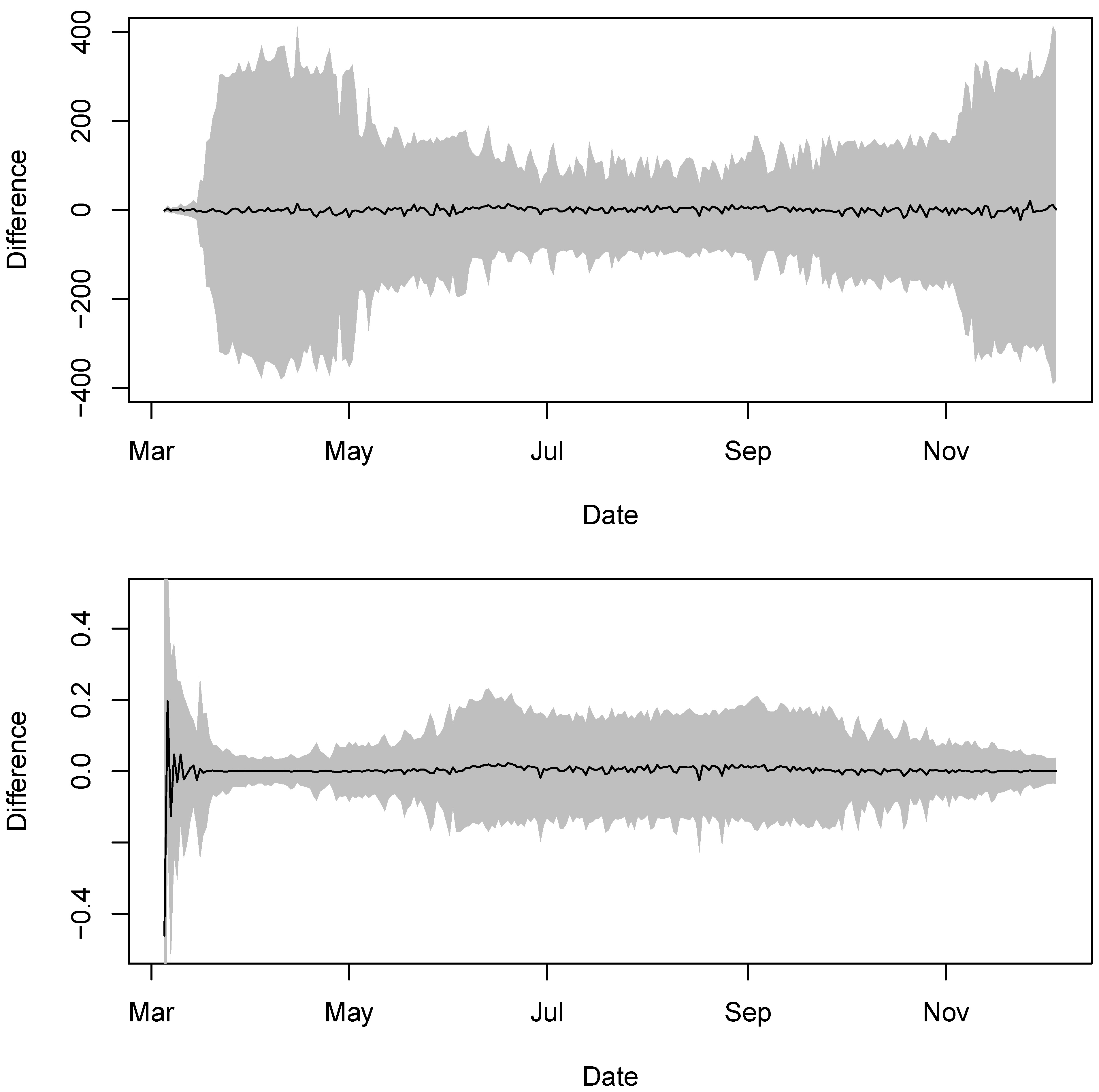
A TV-Pois-AR model was applied without the fix effect,  X β , because we do not have scientific information about any potential covariates. By setting a maximum order of 5, order 2 was considered as the best based on DIC and WAIC. The difference between the estimated exponential of the intensity parameter,  exp ( λ t ) , and the observed series is shown in Figure 5. Figure 6 shows the estimated parameters. Table 3 shows the model selection results. A series of restrictions in New York State began on 3/12/2020, and a state-wide stay-at-home order was declared on 3/20/2020. The number of new cases reached its peak about two weeks after the lockdown. In Figure 6, the first dashed line in the first two plots denotes 3/20/2020, the time when the state-wide stay-at-home order was declared. We can see that the estimated autoregressive coefficients keep changing significantly after this date. This change in the autoregressive coefficients coincides with the lockdown process. The second dashed line in the first two plots denotes 9/26/2020. On that day, the number showed an uptick in cases, with more than 1000 daily COVID-19 cases, which was the first time since early June. About two weeks before this date, the coefficients show some evidence of pattern change. This may be an indication that the lockdown affected the spread of COVID-19. The innovation variance of the intensity is becoming smaller and smaller, probably due to the improvement in testing and reporting. The dashed line in the third plot denotes the date when the peak number of new cases occurred. Since then, the innovation variance has stabilized at a low level.
To evaluate the performance of forecasting, we conducted a rolling one-day-ahead prediction and compared the mean squared prediction errors (MSPE). We picked a starting date and made a one-day-ahead prediction based on the data up to this date. Then, we moved to the next day and made a one-day-ahead prediction based on the data up to the new date. By repeating this until one day before the last day, we obtained the rolling one-day-ahead prediction. Additionally, we conducted a 20-day prediction to evaluate the performance of the long-term forecast.
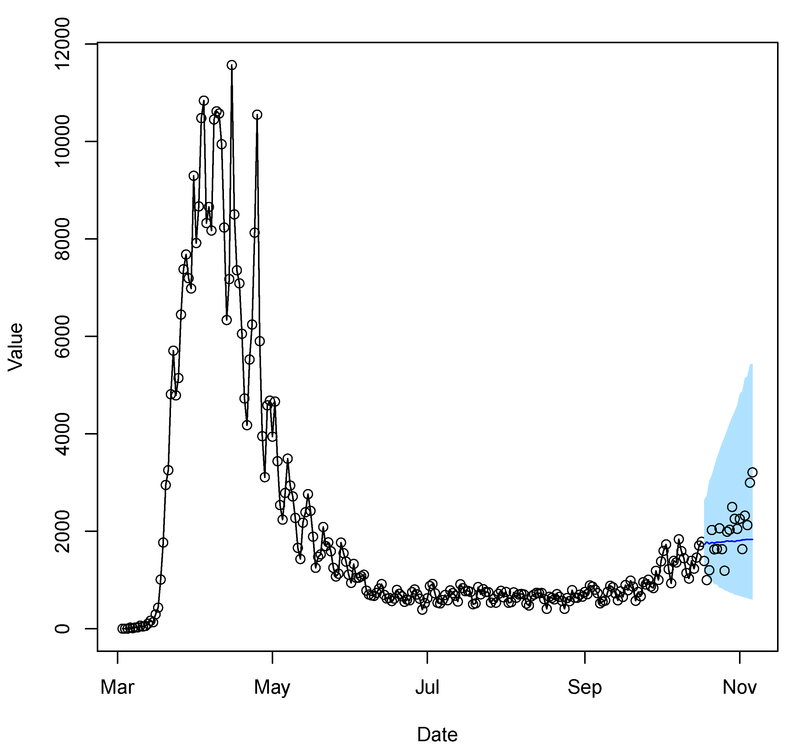
We compare the forecast performance of four methods, where Naive denotes the naive forecast; that is, using the previous period to forecast for the next period (carry-forward). The average MSPE over these days is used for comparison. Table 4 presents the performance of the rolling one-day-ahead prediction. The TV-Pois-AR forecasting outperforms the two existing models and the Naive forecasting. Figure 7 shows an example of a 20-day forecast of the daily new COVID-19 cases from 10/18/2020 to 11/6/2020 in New York State. The example demonstrates how the TV-Pois-AR model captures the time-varying trend.

4.2. Case Study 2: COVID-19 hospitalization in the U.S.

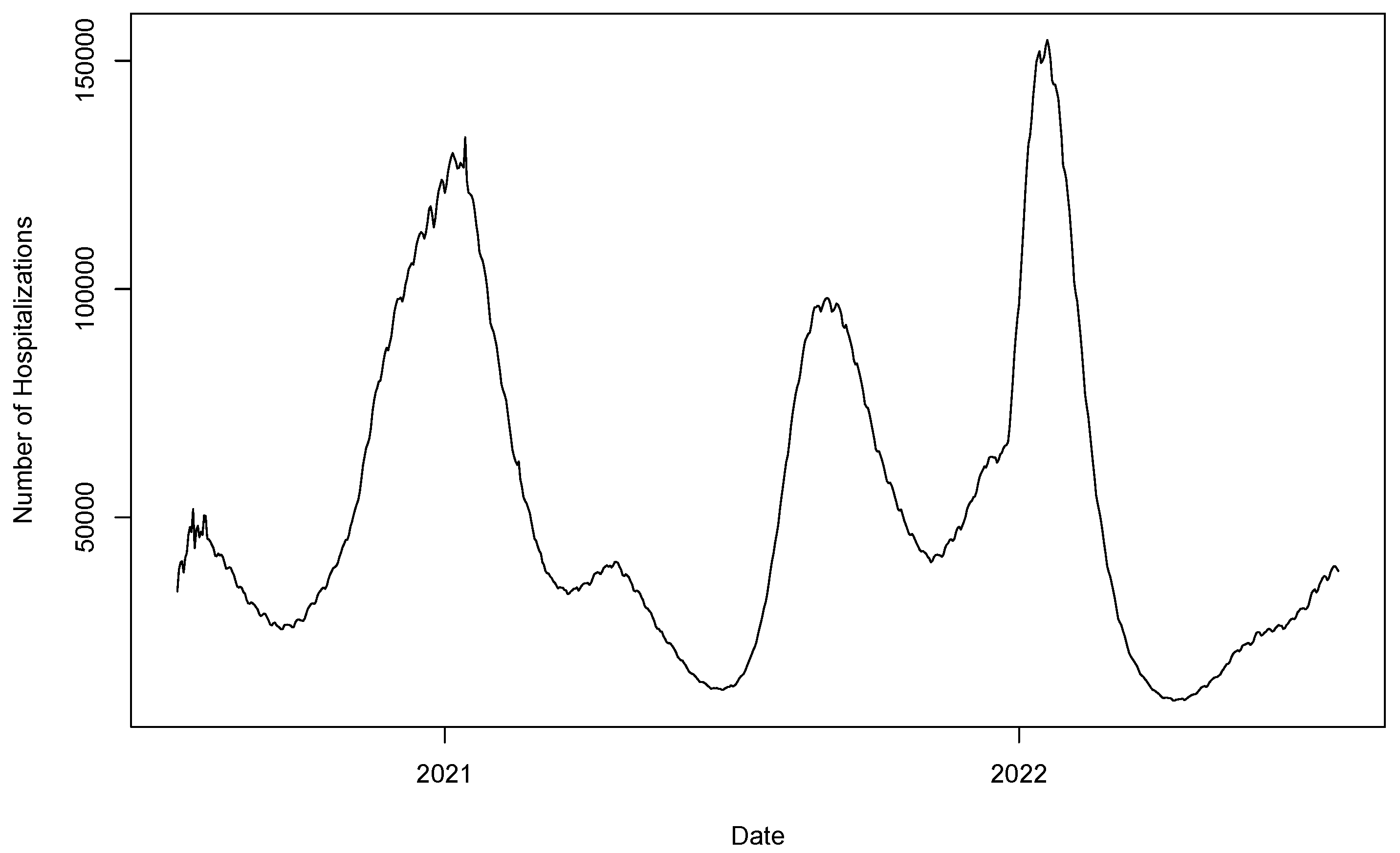
Since the number of daily new COVID-19 cases is no longer systematically collected (starting from early 2022), we use the 739 daily numbers of COVID-19 patients in hospitals in the US from 7/15/2020 to 7/23/2022 (shown in Figure 8) from Our World in Data (https://ourworldindata.org/ (accessed on 11/29/2022)) as another data example. A TV-Pois-AR model is applied, with the model order selected based on DIC and WAIC. By setting a maximum order of 10, order 4 is considered the best, as shown in Table 5. To evaluate the forecasting performance, we make a rolling one-day-ahead prediction and compare the mean squared prediction error (MSPE), as in Case Study 1. The rolling prediction start dates are from 8/19/2021 to 6/14/2022. We compare the forecast performance of four methods, as in Case Study 1. Table 6 shows the rolling one-day-ahead forecast performance of each method in terms of MSPE over the rolling observed COVID data.

5. Discussion

We develop a novel hierarchical Bayesian model to model the nonstationary count time-varying models and propose an efficient estimation approach using an MCMC sampling scheme with embedded NUTS algorithm. We also provide a model selection method by which to choose the discount factors and the optimal model order. The simulation cases show that the parameter estimates have a small mean squared error that, as expected, decreases as the sample size increases. The data example shows that the time-varying coefficients and innovation covariance can reveal the changing pattern over time. The proposed method can be applied not only to the confirmed cases of COVID-19 but also to the number of deaths, number of recovered cases, number of critical cases, and many other parameters for different diseases. Such studies may provide important insights into the spread and the measures required.
The current study is limited to univariate nonstationary count-valued time series. One subject for future research is an extension of the model to multivariate and/or spatiotemporal cases by adding some region-specific effects and jointly modeling the series in multiple regions. Modeling multivariate count-valued time series data is an important research topic in ecology and climatology. Moreover, regarding univariate applications on epidemic disease data, we can consider different government interventions as covariates, which usually have an essential impact on the spread of any infectious disease.

Author Contributions

Methodology, Y.S., S.H.H. and W.-H.Y.; software, Y.S. and W.-H.Y.; writing—original draft preparation, Y.S., S.H.H. and W.-H.Y.; writing—review and editing, Y.S., S.H.H. and W.-H.Y. All authors have read and agreed to the published version of the manuscript.

Funding

This research was partially supported by the U.S. National Science Foundation (NSF) under NSF grants SES-1853096 and NCSE-2215168.

Institutional Review Board Statement

Not applicable.

Informed Consent Statement

Not applicable.

Data Availability Statement

Not applicable.

Acknowledgments

We thank the anonymous referees for providing comments that helped improve an earlier version of this article. This article is released to inform interested parties of ongoing research and to encourage discussion. The views expressed on statistical issues are those of the authors and not those of the NSF or U.S. Census Bureau.

Conflicts of Interest

The authors declare no conflict of interest.

Appendix A. Algorithm of Fitting Poisson TV-AR Time Series

To fit a TV-Pois-AR model, we use Gibbs sampling to generate samples from the full conditional distribution of each of the parameters and the latent variables iteratively. After burn-in, the sample distributions of these parameters and latent variables are the estimated posterior distributions. These samples are generated via Gibbs sampling with the following steps:
  • Draw samples of  y = ( y 1 , , y T )  from the full conditional distritbution  p ( y | z , μ , a , σ 2 ) p ( z | y , μ ) p ( y | a , σ 2 )  using a No-U-Turn Sampler [17,18];
  • Use the posterior means of  a  and  σ 2  obtained from the BLF (see Appendix B) as samples, where  a = ( a 1 , , a T )  and  σ 2 = ( σ 1 2 , , σ T 2 ) ;
  • Draw samples of  μ  from the full conditional distribution  p ( μ | z , y ) p ( z | y , μ ) p ( μ )  using a a no-U-turn sampler.

Appendix B. Bayesian Lattice Filter

  • Step 1. Repeat Step 2 for stage  p = 1 , , P ;
  • Step 2. Apply the sequential filtering and smoothing algorithm (see Appendix C) to the prediction errors of last stage,  f t ( p 1 )  and  b t ( p 1 ) , to obtain  α ^ t ( p ) = μ t ( p )  and  σ 2 ^ t ( p ) = s t ( p )  of the forward and backward equations, and the forward and backward prediction errors,  f t ( p )  and  b t ( p ) , for  t = 1 , , T ;
  • Step 3. The posterior mean of  a t  and  σ t 2  are  α ^ t ( P ) = μ t ( P )  and  σ 2 ^ t ( P ) = s t ( P )  obtained from the Pth stage Step 2.

Appendix C. Sequential Filtering and Smoothing Algorithm

The filtering and smoothing algorithm can be obtained for the backward case in a similar manner. For any series, any stage, we denote the posterior distribution at time t as  ( α t | D t ) T ν t ( μ t , C t ) , a multivariate T distribution with  ν t  df, location parameter  μ t , and scale matrix  C t , and  ( σ t 2 | D t ) G ( ν t / 2 , κ t / 2 ) , a gamma distribution with shape parameter  ν t / 2  and scale parameter  κ t / 2 . These parameters can be computed for all t using the filtering equations below. Note that we use  s t = κ t / ν t  to denote the usual point estimate of  σ t 2 f t  in the equation is the forward prediction error. For  t = 2 , , T , we have
μ t = μ t 1 + z t e t , C t = ( R t z t z t q t ) ( s t / s t 1 ) ,
and
ν t = δ ν t 1 + 1 , κ t = δ κ t 1 + s t 1 e t 2 / q t ,
where
e t = f t z t 1 m t 1 , q t = z t 1 R t z t 1 + s t 1 ,
and
z t = R t f t 1 / q t , R t = C t 1 + G t , G t = C t ( 1 β ) / β .
After applying the filtering equations up to T, we compute the full marginal posterior distribution  ( α t | D T ) T ν t ( μ t , T , C t )  and  ( σ t 2 | D T ) G ( ν t , T / 2 , κ t , T / 2 )  through the smoothing equations
μ t , T = ( 1 β ) μ t + β μ t + 1 , T C t , T = [ ( 1 β ) C t + β 2 C t + 1 , T ] ( s t , T / s t ) ν t , T = ( 1 δ ) ν t + δ ν t + 1 , T 1 / s t , T = ( 1 δ ) / s t + δ s t + 1 , T
and  κ t , T = ν t , T s t , T  for  t = T 1 , , 1 .

Appendix D. Forecasting

We can undertake h-step-ahead forecasting by following these steps.
  • For stage p, compute the h-step-ahead predictive distribution of the PARCOR coefficients following [26 ( α p , T + h ( p ) | D T ) N ( μ T ( p ) ( h ) , C T ( p ) ( h ) )  where  μ T ( h ) = μ T ( p )  and  C T ( p ) ( h ) = C T ( p ) + h G T + h ( p )  with  G T + 1 ( p ) = C t ( p ) ( 1 β ) / β ;
  • Draw J samples of  { α p , T + h ( p ) , p = 1 , , P }  from their predictive distribution;
  • For stage p, compute the h-step-ahead predictive distribution of innovation variance following [26]:  ( σ T + h 2 ( p ) | D T ) G ( ν T ( p ) ( h ) / 2 , κ T ( p ) ( h ) / 2 ) , where  ν T ( p ) ( h ) = δ h ν T ( p )  and  κ T ( p ) ( h ) = δ h κ T ( p ) ;
  • For stage p, draw J samples of  σ T + h 2 ( p )  from its predictive distribution
    G ( ν k + ( T 1 ) K ( p ) ( h ) / 2 , κ k + ( T 1 ) K ( p ) ( h ) / 2 ) ;
  • Compute the samples of the AR coefficients  { a p , T + h ( P ) , p = 1 , , P }  through the Durbin–Levinson algorithm from the samples of  { α p , T + h ( P ) , p = 1 , , P } ;
  • The samples of  y T + h  are generated from its predictive distribution, such that
    y T + h ( j ) | y 1 : T , y T : ( T + h 1 ) ( j ) , a T + h ( j ) , σ T + h 2 ( j ) N ( p = 1 P a p , T + h ( j ) y T + h p ( j ) , σ T + h 2 ( j ) ) , j = 1 , , J ,
    where  y T + h p ( j ) = y T + h p  if  h p 0 ;
  • With the samples of  μ  from its posterior distribution, the samples of the h-step-ahead forecast are drawn as
    z T + h ( j ) | y T + h ( j ) , μ ( j ) Pois ( exp ( y T + h ( j ) + μ ( j ) ) ) , j = , , J ;
  • We use the posterior median of  z T + h  obtained through the samples in (A1) as the h-step-ahead forecast.

References

  1. Cox, D.R.; Gudmundsson, G.; Lindgren, G.; Bondesson, L.; Harsaae, E.; Laake, P.; Juselius, K.; Lauritzen, S.L. Statistical analysis of time series: Some recent developments [with discussion and reply]. Scand. J. Stat. 1981, 8, 93–115. [Google Scholar]
  2. Koopman, S.J.; Lucas, A.; Scharth, M. Predicting time-varying parameters with parameter-driven and observation-driven models. Rev. Econ. Stat. 2016, 98, 97–110. [Google Scholar] [CrossRef]
  3. Ferland, R.; Latour, A.; Oraichi, D. Integer-valued GARCH process. J. Time Ser. Anal. 2006, 27, 923–942. [Google Scholar] [CrossRef]
  4. Fokianos, K.; Rahbek, A.; Tjøstheim, D. Poisson autoregression. J. Am. Stat. Assoc. 2009, 104, 1430–1439. [Google Scholar] [CrossRef]
  5. Al-Osh, M.; Alzaid, A.A. First-order integer-valued autoregressive (INAR (1)) process. J. Time Ser. Anal. 1987, 8, 261–275. [Google Scholar] [CrossRef]
  6. Zeger, S.L. A regression model for time series of counts. Biometrika 1988, 75, 621–629. [Google Scholar] [CrossRef]
  7. Dunsmuir, W.T. Generalized Linear Autoregressive Moving Average Models. In Handbook of Discrete-Valued Time Series; Chapman & Hall/CRC: Boca Raton, FL, USA, 2016; p. 51. [Google Scholar]
  8. Brandt, P.T.; Williams, J.T. A linear Poisson autoregressive model: The Poisson AR (p) model. Political Anal. 2001, 9, 164–184. [Google Scholar] [CrossRef]
  9. Davis, R.A.; Holan, S.H.; Lund, R.; Ravishanker, N. (Eds.) Handbook of Discrete-Valued Time Series; Chapman & Hall/CRC: Boca Raton, FL, USA, 2016. [Google Scholar]
  10. Davis, R.A.; Fokianos, K.; Holan, S.H.; Joe, H.; Livsey, J.; Lund, R.; Pipiras, V.; Ravishanker, N. Count time series: A methodological review. J. Am. Stat. Assoc. 2021, 116, 1533–1547. [Google Scholar] [CrossRef]
  11. Smith, R.; Miller, J. A non-Gaussian state space model and application to prediction of records. J. R. Stat. Soc. Ser. B (Methodol.) 1986, 48, 79–88. [Google Scholar] [CrossRef]
  12. Brandt, P.T.; Williams, J.T.; Fordham, B.O.; Pollins, B. Dynamic modeling for persistent event-count time series. Am. J. Political Sci. 2000, 44, 823–843. [Google Scholar] [CrossRef]
  13. Berry, L.R.; West, M. Bayesian forecasting of many count-valued time series. J. Bus. Econ. Stat. 2019, 38, 872–887. [Google Scholar] [CrossRef]
  14. Bradley, J.R.; Holan, S.H.; Wikle, C.K. Computationally efficient multivariate spatio-temporal models for high-dimensional count-valued data (with discussion). Bayesian Anal. 2018, 13, 253–310. [Google Scholar] [CrossRef]
  15. Bradley, J.R.; Holan, S.H.; Wikle, C.K. Bayesian hierarchical models with conjugate full-conditional distributions for dependent data from the natural exponential family. J. Am. Stat. Assoc. 2020, 115, 2037–2052. [Google Scholar] [CrossRef]
  16. Yang, W.H.; Holan, S.H.; Wikle, C.K. Bayesian lattice filters for time–varying autoregression and time–frequency analysis. Bayesian Anal. 2016, 11, 977–1003. [Google Scholar] [CrossRef]
  17. Hoffman, M.D.; Gelman, A. The No-U-Turn sampler: Adaptively setting path lengths in Hamiltonian Monte Carlo. J. Mach. Learn. Res. 2014, 15, 1593–1623. [Google Scholar]
  18. Märtens, K. HMC No-U-Turn Sampler (NUTS) Implementation in R. 2017. Available online: https://github.com/kasparmartens/NUTS (accessed on 27 July 2020).
  19. Neal, R.M. An improved acceptance procedure for the hybrid Monte Carlo algorithm. J. Comput. Phys. 1994, 111, 194–203. [Google Scholar] [CrossRef]
  20. Neal, R.M. MCMC using Hamiltonian dynamics. In Handbook of Markov Chain Monte Carlo; Chapman & Hall/CRC: Boca Raton, FL, USA, 2011; Volume 2, p. 2. [Google Scholar]
  21. Duane, S.; Kennedy, A.D.; Pendleton, B.J.; Roweth, D. Hybrid Monte Carlo. Phys. Lett. B 1987, 195, 216–222. [Google Scholar] [CrossRef]
  22. Martino, L.; Yang, H.; Luengo, D.; Kanniainen, J.; Corander, J. A fast universal self-tuned sampler within Gibbs sampling. Digit. Signal Process. 2015, 47, 68–83. [Google Scholar] [CrossRef]
  23. Shumway, R.H.; Stoffer, D.S. Time Series Analysis and Its Applications, 2nd ed.; Springer: Berlin/Heidelberg, Germany, 2006. [Google Scholar]
  24. Kitagawa, G. Introduction to Time Series Modeling; Chapman & Hall/CRC: Boca Raton, FL, USA, 2010. [Google Scholar]
  25. Hayes, M.H. Statistical Digital Signal Processing and Modeling; John Wiley & Sons: Hoboken, NJ, USA, 1996. [Google Scholar]
  26. West, M.; Harrison, J. Bayesian Forecasting and Dynamic Models, 2nd ed.; Springer: Berlin/Heidelberg, Germany, 1997. [Google Scholar]
  27. Spiegelhalter, D.J.; Best, N.G.; Carlin, B.P.; Van Der Linde, A. Bayesian measures of model complexity and fit. J. R. Stat. Soc. Ser. B (Stat. Methodol.) 2002, 64, 583–639. [Google Scholar] [CrossRef]
  28. Gelman, A.; Carlin, J.B.; Stern, H.S.; Dunson, D.B.; Vehtari, A.; Rubin, D.B. Bayesian Data Analysis; Chapman & Hall/CRC: Boca Raton, FL, USA, 2013. [Google Scholar]
  29. Watanabe, S. Asymptotic equivalence of Bayes cross validation and widely applicable information criterion in singular learning theory. J. Mach. Learn. Res. 2010, 11, 3571–3594. [Google Scholar]
  30. Watanabe, S. A widely applicable Bayesian information criterion. J. Mach. Learn. Res. 2013, 14, 867–897. [Google Scholar]
  31. Rosen, O.; Stoffer, D.S.; Wood, S. Local spectral analysis via a Bayesian mixture of smoothing splines. J. Am. Stat. Assoc. 2009, 104, 249–262. [Google Scholar] [CrossRef]
  32. Pan, W. Akaike’s information criterion in generalized estimating equations. Biometrics 2001, 57, 120–125. [Google Scholar] [CrossRef] [PubMed]
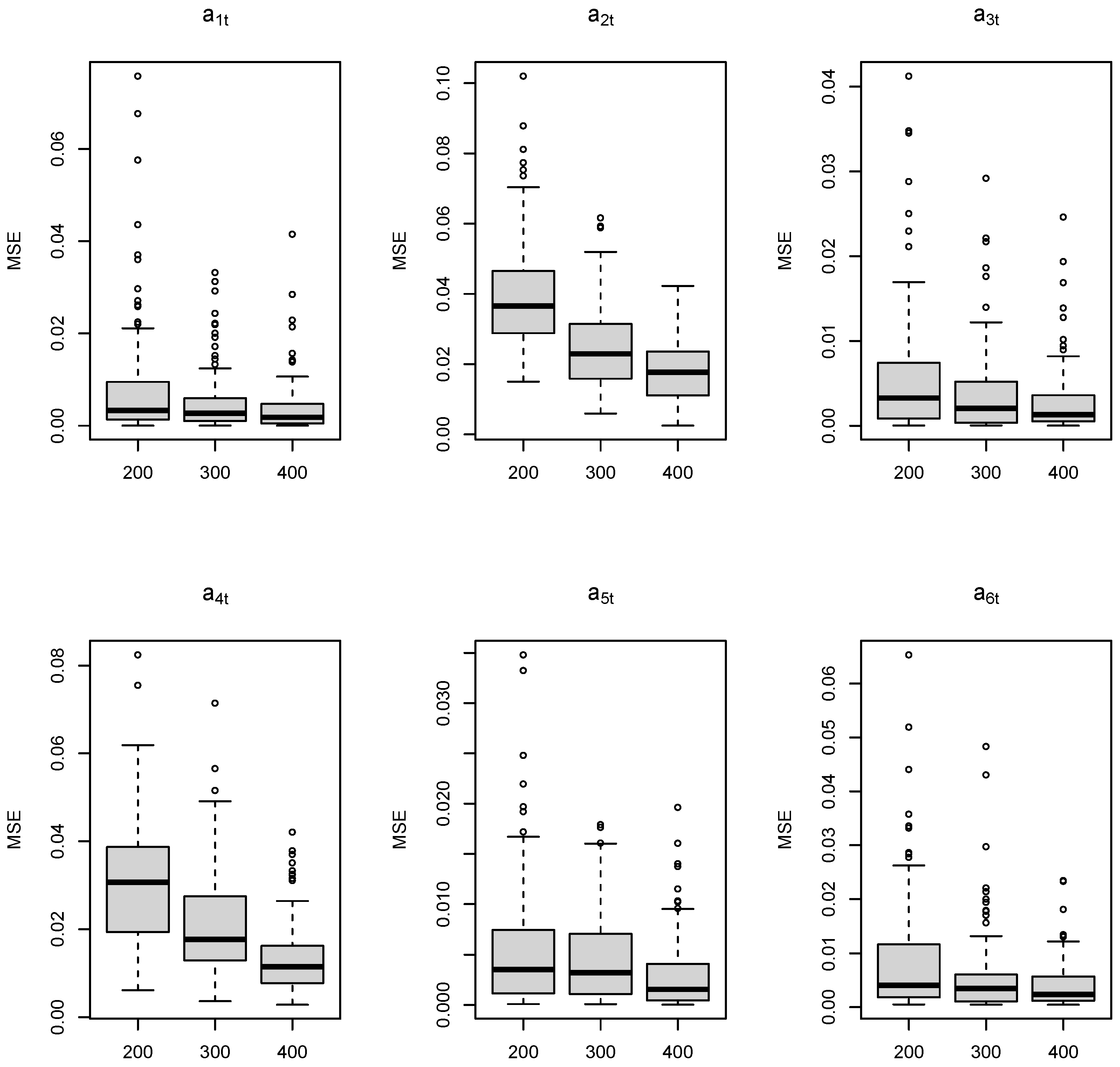
Figure 1. Boxplots of the MSEs of each of the six time-varying coefficients  a 1 , t  through  a 6 , t  for 100 simulated datasets of different lengths: 200, 300, 400.
Stats 06 00065 g001
Figure 2. Boxplots of the MSEs of the intensity and the parameters in the latent process for 100 simulated datasets of different lengths. For each of them, three boxplots of length  200 , 300 , 400  are put side by side from left to right. The left plot shows the MSEs of the innovation variance. The middle plot shows the MSEs of the mean level  μ . The right plot shows the MSEs of the latent variable  y .
Stats 06 00065 g002
Figure 3. The mean and  90 %  pointwise credible intervals of estimated intensity over 100 simulated datasets using different methods. The blue line denotes the estimated values, and the band denotes  90 %  pointwise credible intervals. The red line denotes the true values of intensity. Note that “pointwise credible intervals" are calculated from 100 point estimates independently at each time.
Stats 06 00065 g003
Figure 4. Boxplots of MSE of the estimated intensity over 100 simulated datasets using different methods. Note that the scales of the three boxplots are different.
Stats 06 00065 g004
Figure 5. The difference between daily new COVID-19 cases in New York State and the estimated expected values. The black line is the difference and the grey region shows the corresponding  90 %  credible intervals. The top plot shows the difference in the original scale and the bottom plot shows the difference in the log scale.
Stats 06 00065 g005
Figure 6. The estimated  a 1 , t a 2 , t , and  σ t 2  of the Poisson TV-VAR(2) model applied to daily new COVID-19 cases in New York State from top to bottom, respectively. The grey region shows the corresponding  90 %  credible intervals.
Stats 06 00065 g006
Figure 7. The 20-day forecast of the daily new COVID-19 cases of the last 20 days in New York State. The black overplotted points and lines are the observed daily new cases used for model fitting from 3/3/2020 to 10/17/2020. The black dots are the true daily new cases in the forecast region from 10/18/2020 to 11/6/2020. The blue line shows the 20-day forecast. The light blue region is the  90 %  prediction interval.
Stats 06 00065 g007
Figure 8. The daily number of COVID-19 patients in hospital in the US.
Stats 06 00065 g008
Table 1. Average and standard deviation (s.d.) of MSEs of each of the six time-varying coefficients  a 1 , t  through  a 6 , t  for 100 simulated datasets of different length: 200, 300, 400.s.
Average of MSEs (s.d. of MSEs)
200300400
  a 1 t 0.0086 (0.0136)0.0055 (0.0070)0.0040 (0.0063)
  a 2 t 0.0404 (0.0165)0.0254 (0.0119)0.0183 (0.0083)
  a 3 t 0.0061 (0.0080)0.0039 (0.0052)0.0030 (0.0042)
  a 4 t 0.0307 (0.0139)0.0212 (0.0121)0.0136 (0.0086)
  a 5 t 0.0058 (0.0068)0.0047 (0.0047)0.0031 (0.0039)
  a 6 t 0.0091 (0.0117)0.0058 (0.0081)0.0044 (0.0049)
Table 2. Average mean squared error (AMSE) of the estimated intensity over the 100 simulated datasets using different methods.
ModelINGARCHGLARMATV-Pois-AR
AMSE597,041.3621,732.52568.6
Table 3. Model selection of Poisson TV-AR model for the daily new COVID-19 cases in New York State. Each column gives the model order P and the value of the model selection criteron.
P12345
DIC1738.5401735.7481783.4841779.9461796.255
WAIC303.004295.531317.326316.626320.476
Table 4. One-step-ahead predictive performance of TV-Pois-AR(2) and other models on COVID-19 data in New York State from 7/19/2020. There are two start dates for the rolling predictions.
ModelMPSE
TV-Pois-AR(2)2.277 × 10 5
GLARMA(6,2)2.363 × 10 5
INGARCH(1,0)2.675 × 10 5
Naive2.286 × 10 5
Table 5. Model selection of Poisson TV-AR model for the daily COVID-19 hospitalization in the U.S. Each column gives the model order P and the value of the model selection criteron.
P12345
DIC24,481.3923,898.0723,248.0822,726.5823,278.76
WAIC6518.816190.7465863.4225612.3375881.701
Table 6. Percentage of TV-Pois-AR(4) giving better forecasts of one-step-ahead rolling predictions on US COVID-19 hospitalization data from 11/27/2021 to 9/22/2022. The posterior medians of the future observations are used as the forecast values.
ModelMSPE
Pois-TVAR1.51 × 10 6
GLARMA(6,2)16.00 × 10 6
INGARCH(1,0)11.10 × 10 6
Naive3.20 × 10 6
Disclaimer/Publisher’s Note: The statements, opinions and data contained in all publications are solely those of the individual author(s) and contributor(s) and not of MDPI and/or the editor(s). MDPI and/or the editor(s) disclaim responsibility for any injury to people or property resulting from any ideas, methods, instructions or products referred to in the content.