Omnibus Tests for Multiple Binomial Proportions via Doubly Sampled Framework with Under-Reported Data

Abstract

Previously, Rahardja (2020) paper (in the first reference list) developed a (pairwise) multiple comparison procedure (MCP) to determine which (proportions) pairs of Multiple Binomial Proportions (with under-reported data), the significant differences came from. Generally, such an MCP test (developed by Rahardja, 2020) is the second part of a two-stage sequential test. In this paper, we derived two omnibus tests (i.e., the overall equality of multiple proportions test) as the first part of the above two-stage sequential test (with under-reported data), in general. Using two likelihood-based approaches, we acquire two Wald-type (Omnibus) tests to compare Multiple Binomial Proportions (in the presence of under-reported data). Our closed-form algorithm is easy to implement and not computationally burdensome. We applied our algorithm to a vehicle-accident data example.

1. Introduction

As stated in the Abstract, this paper is the continuation of Rahardja (2020) paper [1]. In regard to counts-and-proportions (categorical) type of data, the topic of interest here is about miscategorization of categorical data, particularly, binomial outcome data. For example, counts of disease/no-disease cancer screening in a hospital, proportions of male/female vehicle-driver accidents in an insurance company, counts of correct/incorrect audited payments in an accounting firm, etc. In an ideal (error-free) world, there is no miscategorization. Then, the simple and straightforward estimators (counts-and-proportions) taught in an introductory statistics (Stat 101) course can just be applied. However, the fact that in this imperfect world, errors or flaws (miscategorization) exist and cannot be ignored because such presence of under-reported or over-reported errors may create severe bias [2,3]. The fact that such imperfections exist in this world (due to the presence of under-reported or over-reported errors) is the motivation behind this research: to remedy the bias by incorporating a doubly sampled framework and to achieve model identifiability. Consequently (as a brief overview), our objective here is to provide a (bias remedy) method, by using a doubly sampled framework, in the presence of either under-reported or over-reported data. In the next paragraphs, we will go over the bibliography and novelty of this research.

In reality, we frequently run into data structure of a binomial output variable and a nominal input variable with multiple groups or levels, within that nominal input variable. In the scenario that both the binomial output variable and the nominal input variable are perfectly counted with no mistake, one can just use the Pearson chi-square statistics (taught in a Stat 101 course) to test the relationship between the input and output variables. Nevertheless, there are data cases where the nominal input variable (for example, a patient-category nominal input variable with g = 3 levels: male/female/pediatric) is categorized flawlessly with no error, while the binomial/binary output variable (e.g., disease/no-disease) is categorized using an error-prone classifier. Such error-prone classifier can misclassify a disease-free (male/female/pediatric) patient into disease output category and vice versa. Therefore, the objective is to examine whether there is any relationship between the nominal input variable (patient-category, with three levels: male/female/pediatric) and the binomial output variable. In other words, to test if the patient-category matters (i.e., testing whether the proportions of the three patient-category are the same, hence, H₀: p_male = p_female = p_pediatric) in determining the output (disease-free/not). Among many past research, Bross in 1954 [2] and Goldberg in 1975 [3] examined that with error-prone classifier, the bias can be severe, in their case of determining the odds ratio for misclassified binomial data with two levels (g = 2) of input variables. Subsequently, to adjust for the bias, a sampling framework is needed to obtain valid estimators.

In the case that an error-free classifier is also accessible for acquiring the binomial output variable, one can use a doubly sampled framework, pioneered by Tenenbein in 1970 [4], to reach model identifiability and to remedy bias. Here, is how the doubly sampled framework operates. First, one chooses either an arbitrary subset from the main data or another new sample. In the former scenario where one chooses an arbitrary subset from the main data, the error-free classifier is utilized to attain the correct measurement of the binomial output variable for such subset. In the second scenario, one chooses another new sample, and utilize both the error-prone and the error-free classifier to attain the binomial output variable for such new sample. Additionally, one also measures the nominal input variable for this new sample. To put it another way, the subset or new sample can contain three categorical variables: a nominal input variable measured with no error, a miscategorized output variable by the error-prone classifier, and an output variable measured with no error by the error-free classifier. In both scenarios, we designate the sample categorized only by the error-prone classifier for the binomial output variable as the original study and the sample categorized by both the error-prone and error-free classifiers for the binomial output variable as the validation substudy. Then, we combine the original study and the validation substudy to be the overall data, where the inferential statistics are based on.

There are a lot of bibliography for g equals 1 or 2 (but not for g ≥ 3). When g = 1 and only over-reported or under-reported data exists, Moors et al. in 2000 [5] proposed a one-sided exact confidence interval and Boese et al. in 2006 [6] devised several likelihood-based confidence intervals (CIs) for the proportion parameter. Moreover, Raats and Moors in 2003 [7] and Lee and Byun in 2008 [8] considered Bayesian credible intervals for the proportion parameter. When g = 1 and both over-reported and under-reported data exist, Raats and Moors in 2003 [7] obtained both an exact confidence interval and a Bayesian credible set for the proportion parameter while Lee in 2013 [9] offered a Bayesian approach. When g = 2 with only over-reported or under-reported data, Rahardja et al. derived both Bayesian in 2019 [10] and Likelihood-Based inference in 2019 [11] for the difference of two proportion parameters. For g = 2 with both over-reported and under-reported data, Prescott and Garthwaite in 2002 [12] offered Bayesian credible interval; while Morrissey and Spiegelman in 1999 [13] presented likelihood-based confidence intervals for the odds ratio.

Usually, we encounter both over-reported and under-reported data at the same time. However, occasionally data also exist for only over-reported or only under-reported. From the existing bibliography, the statistical methods derivation and the corresponding computing-algorithm developments are different and cannot be used automatically for either type of misclassifications. Hence, it is necessary to specifically derive different method for each type of misclassification. To date, the bibliography only presented methods for g = 1 with only one error type (over-/under-reported only); g = 1 for both error types; g = 2 with only one error type (over-/under-reported only); g = 2 for both error types; moreover, all their algorithms are non-closed form (except, in all the aforementioned Rahardja et al. [10,11] papers, where algorithms were closed-form) and hence, their algorithms encountered a lot of computational difficulties, hard to reproduce, and computationally very burdensome.

Therefore, in light of novelty, in this article, we propose two likelihood-based (two Wald-type Omnibus Testing: naïve and modified) methods to analyze data obtained via a doubly sampled framework for g ≥ 3. Without loss of generality (WLOG), here we limit the scope of our omnibus testing methods to only one error type (under-reported or over-reported only) data. Again, the objective is to test the relationship between the nominal input variable (with multiple levels or groups) and the binomial output variable. Equivalently, this objective translates into H₀: p₁ = p₂ = … = p_g, or testing the equality of the multiple binomial proportions among g groups (i.e., the equality of the levels of this nominal input variable). If the proportions are not significantly different, i.e., H₀ is not rejected, then there is no relationship between the nominal input variable and the binomial output variable. Vice versa, if H₀ is rejected, then there is relationship. The rest of the article is managed (described) this way. In Section 2 we lay down the data structure. In Section 3 we formulate two omnibus tests (Wald-type) statistics to test the relationship between the two variables (input and output). In Section 4, as an example, we demonstrate our two omnibus tests by employing real data. In Section 5 we assess the Type I error rates and power of the tests via simulations. Finally, in Section 6, we present the conclusion, limitations, and future research.

2. Data Structure

In this section, we consider multiple-sample binomial data with only under-reported data obtained using a doubly sampled framework. Since there has been various discussion and methods proposed in the literature, for g = 1 and g = 2, here we provide a description of the kind of data structure that has been discussed (see

Table 1. Data for group i.

Study	Error-Free Classifier	Error-Prone Classifier
		0	1	Total
Validation	0	ni00	ni01	ni0∙
	1	NA	ni11	ni11
	Total	ni00	ni∙1	ni
Original	NA	yi	xi	mi

NA: Not Available.

for such data structure under consideration) and generalized it to g ≥ 3 scenario.

As previously mentioned in Section 1, for each of the g groups, the overall data structure is composed of two independent datasets: the original study and the validation substudy. Due to economic viability, one only utilizes the perfect classifier in the validation substudy; while using the imperfect classifier in both the original and validation studies. We exhibit the summary counts in both the original and the validation studies for the data structure in Table 1. We let the size of observations m_i and n_i in both the original and the validation studies, for each group i (i = 1, …, g), respectively. We then define N_i = m_i + n_i be the total number of units for group i.

In the original study, we define x_i and y_i be the numbers of positive and negative classifications in group i using the error-prone classifier. In the validation study (for i = 1, …, g, j = 0, 1, and k = 0, 1), we denote n_ijk as the sample size in group i classified as j and k using the error-free and the error-prone classifiers, respectively.

Here, we have more notations to define. For the jth unit in the ith group, while i = 1, …, g and j = 1, …, N_i, we designate F_ij and T_ij as the binomial output variables for the error-prone and error-free classifiers, respectively. Note that both F_ij and T_ij are observable for all units in both the original and the validation studies, while T_ij is only observable units in the validation substudy. If the result is positive by the error-prone classifier, we mark F_ij = 1; else, F_ij = 0. Likewise, we mark T_ij = 1 if the result is truly positive using the error-free classifier; else, T_ij = 0. Clearly, misclassification occurs when F_ij ≠ T_ij.

Next, we mark the parameters for group i as follows. Again, in this article, WLOG we consider under-reported data only, since the same formulation generality will apply (to over-reported only), as well. We let the true proportion parameters of interest be $p_i=\mathrm{Pr}(T_{ij}=1)$, the proportion parameters of the error-prone classifier be ${\pi }_i=\mathrm{Pr}(F_{ij}=1)$, and the false positive rates of the error-prone classifier be ${\phi }_i=\mathrm{Pr}(F_{ij}=1|T_{ij}=0)$ for i = 1, 2, …, g. Note that π_i is not an additional unique parameter because it is obtainable by using all other parameters. In particular, using the law of total probability, we have

$${\pi }_i=\mathrm{Pr}(T_{ij}=1)\mathrm{Pr}(F_{ij}=1|T_{ij}=1)+\mathrm{Pr}(T_{ij}=0)\mathrm{Pr}(F_{ij}=1|T_{ij}=0)=p_i+q_i{\phi }_i,$$

(1)

where q_i = 1 − p_i. In relation to the summary counts arranged in Table 1, we exhibit the associated cell probabilities in

Table 2. Cell probabilities for group i.

Study	Error-Free Classifier	Error-Prone Classifier
		0	1	Total
Validation	0	qi (1 − φi)	qi φi	qi
	1	NA	pi	pi
Original	NA	1 − πi	πi	1

NA: Not Available.

.

Our goal is to test the relationship between the categorical (nominal) input variable and the (binomial) output variable. In other words, whether the levels within the (nominal) input variable matters (testing equal proportions), in predicting the binomial output variable. In particular, the statistical hypotheses of interest can be written as

$$H_0:p_1=p_2=\dots =p_g\mathrm{vs.}{H}_1:\mathrm{at}\mathrm{least}\mathrm{one}\mathrm{pair}\mathrm{is}\mathrm{not}\mathrm{equal}.$$

(2)

Again, this goal translates into testing the equality of the multiple binomial proportions among g groups (i.e., if the proportions are not significantly different, or H₀ is not rejected, then there is no relationship between the categorical (nominal) input variable and the binomial output; and vice versa, if H₀ is rejected, then there is association).

3. Methods

In this section we aim to derive two (omnibus) statistical tests for testing the hypotheses in Expression (2). We begin with estimating the Maximum Likelihood Estimator (MLE) along with its asymptotic variance-covariance matrix for every single one of the parameters based on the full-likelihood function. Next, we acquire two chi-square tests for testing the Expression (2) where the second test is essentially an improved version of the first test.

3.1. The Maximum Likelihood Estimator (MLE)

We display the data structure under consideration in Table 1. For group i, the observed counts $(n_{i00},n_{i01},n_{i11})$ from the validation substudy have a Trinomial distribution with total size n_i and associated probabilities displayed in an upper right 2 × 2 submatrix in Table 2, i.e.,

$$(n_{i00},n_{i01},n_{i11})|p_i,{\phi }_i~\mathrm{Trinomial}\left[n_i,\left(q_i(1-{\phi }_i),q_i{\phi }_i,p_i\right)\right].$$

Note that Multinomial Distribution [14] is the generalization of Binomial [15] distribution. Trinomial Distribution [16] is another special case of Multinomial Distribution [14]. Moreover, the observed counts (x_i, y_i) in the original study have the following binomial distribution:

$$(x_i,y_i)|p_i,{\phi }_i~\mathrm{Bin}\left[m_i,\left({\pi }_i,1-{\pi }_i\right)\right].$$

Since $(n_{i00},n_{i01},n_{i11})$ and $(x_i,y_i)$ are independent for group i and these cell counts are independent across groups, up to a constant, the full-likelihood function is

$$L(\eta )={\displaystyle \prod _{i=1}^g\left\{{\left[q_i\left(1-{\phi }_i\right)\right]}^{n_{i00}}{\left[q_i{\phi }_i\right]}^{n_{i01}}{p}_i{}^{n_{i11}}{\pi }_i^{x_i}{\left(1-{\pi }_i\right)}^{y_i}\right\}},$$

(3)

where $\eta =\left(p_1,{\phi }_1,\dots ,p_g,{\phi }_g\right)$ is the parameter vector.

Directly maximizing (3) with respect to η is not straightforward. Instead of using numerical methods or non-closed form algorithm (which have been the historical challenges in the bibliography), we use a reparameterization of η and derive a closed-form solution. Specifically, we newly introduce

$${\lambda }_i=\frac{p_i}{{\pi }_i}.$$

(4)

Then, we introduce the new set of parameters to be a vector $\mathsf{\gamma }=\left({\lambda }_1,{\pi }_1,\dots ,{\lambda }_g,{\pi }_g\right)$. Via Expression (3), the full log likelihood function in γ is

$$l(\mathsf{\gamma })={\displaystyle \sum _{i=1}^g[n_{i11}\log {\lambda }_i+n_{i01}\log \left(1-{\lambda }_i\right)+}\left(x_i+n_{i•1}\right)\log {\pi }_i+\left(y_i+n_{i00}\right)\log \left(1-{\pi }_i\right)].$$

The corresponding score vector has the following form:

$$(\frac{n_{111}}{{\lambda }_1}-\frac{n_{101}}{1-{\lambda }_1},\frac{x_1+n_{1•1}}{{\pi }_1}-\frac{y_1+n_{100}}{1-{\pi }_1},\dots ,\frac{n_{g11}}{{\lambda }_g}-\frac{n_{g01}}{1-{\lambda }_g},\frac{x_g+n_{g•1}}{{\pi }_g}-\frac{y_g+n_{g00}}{1-{\pi }_g}).$$

(5)

By setting the above score vector to 0, we obtain the MLE for γ as a vector ${\widehat{\lambda }}_i=n_{i11}/n_{i•1}$ and ${\widehat{\pi }}_i=(x_i+n_{i•1})/N_i$. By solving Expressions (1) and (4) and applying the invariance property of MLE, the MLE for the vector η is ${\widehat{p}}_i={\widehat{\pi }}_i{\widehat{\lambda }}_i$ and ${\widehat{\phi }}_i=(1-{\widehat{\lambda }}_i){\widehat{\pi }}_i/{\widehat{q}}_i.$

Using Expression (5), the expected Fisher information matrix $I(\mathsf{\gamma })$ is computed as a diagonal matrix with the following diagonal elements:

$$\left(\frac{n_1{\pi }_1}{{\lambda }_1(1-{\lambda }_1)},\frac{N_1}{{\pi }_1(1-{\pi }_1)},\dots ,\frac{n_g{\pi }_g}{{\lambda }_g(1-{\lambda }_g)},\frac{N_g}{{\pi }_g(1-{\pi }_g)}\right).$$

We can inspect that the regularity conditions are fulfilled for this model. Hence, the MLE $\widehat{\mathsf{\gamma }}=\left({\widehat{\lambda }}_1,{\widehat{\pi }}_1,\dots ,{\widehat{\lambda }}_g,{\widehat{\pi }}_g\right)$ has an asymptotic multivariate normal distribution with mean γ and covariance matrix $I^{-1}(\mathsf{\gamma })$, which is a diagonal matrix with the following diagonal elements:

$$\left(\frac{{\lambda }_1(1-{\lambda }_1)}{n_1{\pi }_1},\frac{{\pi }_1(1-{\pi }_1)}{N_1},\dots ,\frac{{\lambda }_g(1-{\lambda }_g)}{n_g{\pi }_g},\frac{{\pi }_g(1-{\pi }_g)}{N_g}\right).$$

Hence, asymptotically, we have

$$V({\widehat{\lambda }}_i)={\lambda }_i(1-{\lambda }_i)/(n_i{\pi }_i)\mathrm{and}V({\widehat{\pi }}_i)={\pi }_i(1-{\pi }_i)/N_i.$$

Moreover, ${\widehat{\lambda }}_1,{\widehat{\pi }}_1,\dots ,{\widehat{\lambda }}_g,{\widehat{\pi }}_g$ are asymptotically independent.

Since ${\widehat{p}}_i={\widehat{\pi }}_i{\widehat{\lambda }}_i$ and ${\widehat{\lambda }}_i,{\widehat{\pi }}_i$ are asymptotically independent, using the Delta method, the variance of ${\widehat{p}}_i$ can be written as follows:

$${\sigma }_i^2=\frac{{\pi }_i{\lambda }_i(1-{\lambda }_i)}{n_i}+\frac{{\lambda }_i{}^2{\pi }_i(1-{\pi }_i)}{N_i}.$$

A consistent estimator of ${\sigma }_i^2$ is

$${\widehat{\sigma }}_i^2=\frac{{\widehat{\pi }}_i{\widehat{\lambda }}_i(1-{\widehat{\lambda }}_i)}{n_i}+\frac{{\widehat{\lambda }}_i{}^2{\widehat{\pi }}_i(1-{\widehat{\pi }}_i)}{N_i}.$$

3.2. The Two Chi-Square Tests

Here, we present two chi-square tests: the naïve Wald test and the modified Wald test, where the second test is essentially an improved version of the first test. The hypotheses in Expression (2) are equivalent to

$$H_0^{(1)}:Cp=0\mathrm{vs.}{H}_1^{(1)}:\mathrm{Not}{H}_0^{(1)},$$

(6)

where $C=\left[\begin{array}{ccccc}1& -1& 0& \cdots & 0\\ \cdots & \cdots & \cdots & \cdots & \cdots \\ 1& 0& 0& \cdots & -1\end{array}\right]$ and $p=\left(p_1,\dots ,p_g\right)$.

3.2.1. Naïve Wald (nWald) Test

Under Expressions (2) or (6), asymptotically, we have

$$T_1={\left(\mathbf{C}\widehat{\mathbf{p}}\right)}^T{\left(C\widehat{\mathbf{\Sigma }}{C}^T\right)}^{-1}\left(\mathbf{C}\widehat{\mathbf{p}}\right)~{\chi }_{g-1}^2,$$

where $\widehat{\mathbf{p}}=\left({\widehat{p}}_1,\dots ,{\widehat{p}}_g\right)$ and $\widehat{\mathbf{\Sigma }}=\mathrm{diag}({\widehat{\sigma }}_1^2,\dots ,{\widehat{\sigma }}_g^2)$. Hence, we reject the null hypothesis in Expressions (2) or (6) at Type I error level α if $T_1>{\chi }_{g-1,1-\alpha /2}^2$, where ${\chi }_{g-1,1-\alpha /2}^2$ is the $(1-\alpha /2)$ quantile of the chi-square distribution with $g-1$ degrees of freedom. Note that we derive T₁ by applying a naïve Wald test procedure and therefore we name it as a naïve Wald (nWald) test. Such tests are known to be liberal and tend to have Type I error rates above the nominal level.

3.2.2. Modified Wald (mWald) Test

To better refine the naïve Wald test, we utilize $s_i=\mathrm{logit}(p_i)$. The MLE for $s_i$ is ${\widehat{s}}_i=\mathrm{logit}({\widehat{p}}_i)$. Since the range of $s_i$ is the real line, the asymptotic distribution of ${\widehat{s}}_i$ is better approximated by a normal distribution than that of ${\widehat{p}}_i$. Subsequently, in what follows we will construct a test based on ${\widehat{s}}_i$. By the Delta method, we have ${\tau }_i^2\equiv V({\widehat{s}}_i)={\sigma }_i^2/{[p_i(1-p_i)]}^2$. A consistent estimator for ${\tau }_i{}^2$ is ${\widehat{\tau }}_i^2={\widehat{\sigma }}_i^2/{[{\widehat{p}}_i(1-{\widehat{p}}_i)]}^2$.

We note that the hypotheses in Expression (2) are also equivalent to

$$H_0^{(2)}:Cs=0\mathrm{vs.}{H}_1^{(2)}:\mathrm{Not}{H}_0^{(2)},$$

(7)

where $s=\left(s_1,\dots ,s_g\right)$. Now, because under Expressions (2) or (7), asymptotically, we have

$$T_2={\left(\mathbf{C}\widehat{\mathbf{s}}\right)}^T{\left(C\widehat{\mathbf{\Omega }}{C}^T\right)}^{-1}\left(\mathbf{C}\widehat{\mathbf{s}}\right)~{\chi }_{g-1}^2,$$

where $\widehat{\mathbf{s}}=\left({\widehat{s}}_1,\dots ,{\widehat{s}}_g\right)$ and $\widehat{\mathbf{\Omega }}=\mathrm{diag}({\widehat{\tau }}_1^2,\dots ,{\widehat{\tau }}_g^2)$.

We reject the null hypothesis in Expressions (2) or (7) at Type I error level α if $T_2>{\chi }_{g-1,1-\alpha /2}^2$. Such testing method is called the modified Wald (mWald) test.

4. Example

To demonstrate the two Omnibus tests (nWald and mWald) derived in Section 3 of this manuscript (as the First Part/Stage of our Two-Stage Sequential Test), here (for example-continuity purpose), we apply the same vehicle-accident data published by Hochberg in 1977 [17] and demonstrated by Rahardja in 2020 [1] as the Second Part/Stage of our Two-Stage Sequential Testing development.

To recap, the narrative of such vehicle-accident data [1,17] is as follows. There are two classifiers for categorizing accidents into two [output] categories: with injuries (=1) or without injuries (=0). Our error-prone classifier is the police classifier which is prone to error. The other error-free classifier (gold standard) is the non-police classifier which does not miscategorize (e.g., hospital records of injury examination and vehicle-insurance company examination). The original study is based on police reports on vehicle accidents in North Carolina in 1974. The validation substudy is based on accidents that occurred in North Carolina during an unspecified short period in early 1975. The vehicle-accident data are displayed in

Table 3. Vehicle accident data.

Group	Study	Error-Free Classifier	Error-Prone Classifier
			0	1
A (Male and High Vehicle Damage)	Validation	0	369	NA
		1	75	132
	Original	NA	19,631	7329
B (Female and High Vehicle Damage)	Validation	0	123	NA
		1	61	87
	Original	NA	7692	4004
C (Male and Low Vehicle Damage)	Validation	0	529	NA
		1	59	39
	Original	NA	25,542	1886
D (Female and Low Vehicle Damage)	Validation	0	249	NA
		1	43	30
	Original	NA	12,461	1539

NA: Not Available.

.

In such vehicle-accident example [1,17], the objective is to contrast the probability of injury among four (4) groups: Male and High vehicle damage (A), Female and High vehicle damage (B), Male and Low vehicle damage (C), and Female and Low vehicle damage (D). Again, for example and continuity with Rahardja’s manuscript in 2020 [1], we adopt the same Hochberg vehicle-accident data published in 1977 [17] as displayed in Table 3.

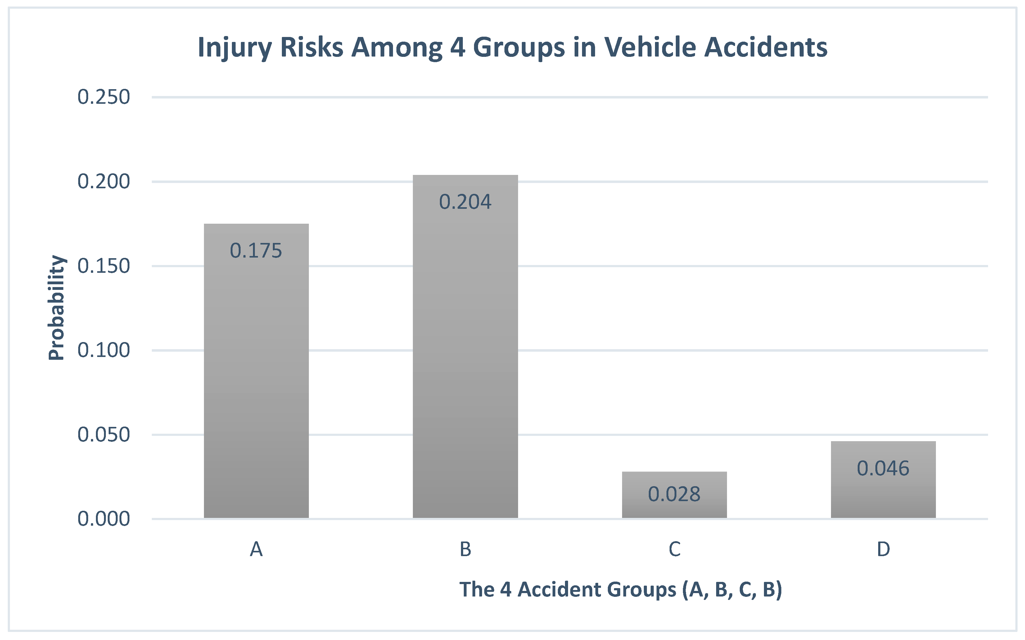
Recall that from Expression (2), the null hypothesis in this context is to test if the chance of injuries among the four (4) accident groups are equal. Using the two (omnibus) tests developed in Section 3, the probabilities of injury for the four groups are obtained as p₁ = 0.175, p₂ = 0.204, p₃ = 0.028, and p₄ = 0.046. The chi-square statistics and p-values for testing the equality of the four proportions are nWald (T₁ = 220.67, p-value < 0.0001) and mWald (T₂ = 143.98, p-value < 0.0001). Since the p-value are less than 0.05 (hence, at the 5% level of significance), we conclude that the vehicle-accident study provided enough statistical evidence in support of an association/relationship between the output (injure risks) and the (nominal) input variable (with four-level of category: A = Male and High vehicle damage, B = Female and High vehicle damage, C = Male and Low vehicle damage, and D = Female and Low vehicle damage) because those risks of injuries (p₁ = 0.175, p₂ = 0.204, p₃ = 0.028, and p₄ = 0.046) are significantly different among those four groups (A, B, C, D). In other words, the four category as levels of input variable matters in predicting the injury risks (4-category). Since there were statistically significant differences among the four-level of input variable, then it is necessary to proceed to the Second Part/Stage (of the Two-Stage Sequential Testing Procedures) to determine which pair(s) contributes the proportions difference. In addition to the numeric version of results described above (in terms of test statistics, p-value, and probabilities of injuries), it is also evidenced from the graphical version of results graphed in Figure 1—visually, the height (probabilities) of the histogram showed significant different among the four accident groups (A, B, C, D). As anticipated, both the numeric and graphical versions of results are consistent in showing that there are significant different among the four accident groups. Such results concluded the First Part/Stage testing (of the Two-Stage Sequential Testing Procedure). Next, one can proceed to the Second Part/Stage testing.

Note again that such Second Part/Stage testing (of the Two-Stage Sequential Testing Procedures) was already completed/demonstrated by Rahardja in 2020 manuscript [1]; and as a summary recap, those significant differences came from the following pairs: AC, AD, BC, and BD.

5. Simulation

In this Simulation Section, we would like to mention that there is no software package and/or library package readily available for such methodology developed above (in Section 3) because generally, the methodology was developed first, before the software package. Then, typically, after a decade or more, when the method developed has become popular then commercial/non-commercial software companies or individuals start building software package and/or library package; not the reverse. Hence, we resorted to writing our own manual coding via R software [18] version 4.1.2. Since the methodologies or algorithm developed above (in Section 3) are closed-form (unlike those non-closed form algorithms formerly developed in all the previous literature reviews), it does not require much/intensive computing resource. Consequently, we can merely utilize a regular laptop/desktop computer. In other words, parallel super computers are not necessary. Here, we use a regular computer with the following specifications: Dual Core Processor of 4GB RAM CPU and a hard drive storage of 1TB; and each case of the simulations we describe below only takes about 2 min to run.

Simulations were performed to evaluate and contrast the performance of nWald and mWald tests under varying cases using empirical Type I error rate. A two-sided nominal-level Type I error rate of α = 0.1 was used for a selection of g = 3 levels. Even though not required by the two tests, for the sake of simplifying the simulation and display of results, equal sample sizes N₁ = N₂ = N₃ = N, substudy sample sizes n₁ = n₂ = n₃ = n, and false-positive (over-reported) rates φ₁ = φ₂ = φ₃ = φ were utilized in simulations. For each simulation configuration, we generated K = 10,000 datasets.

5.1. Type I Error Rate

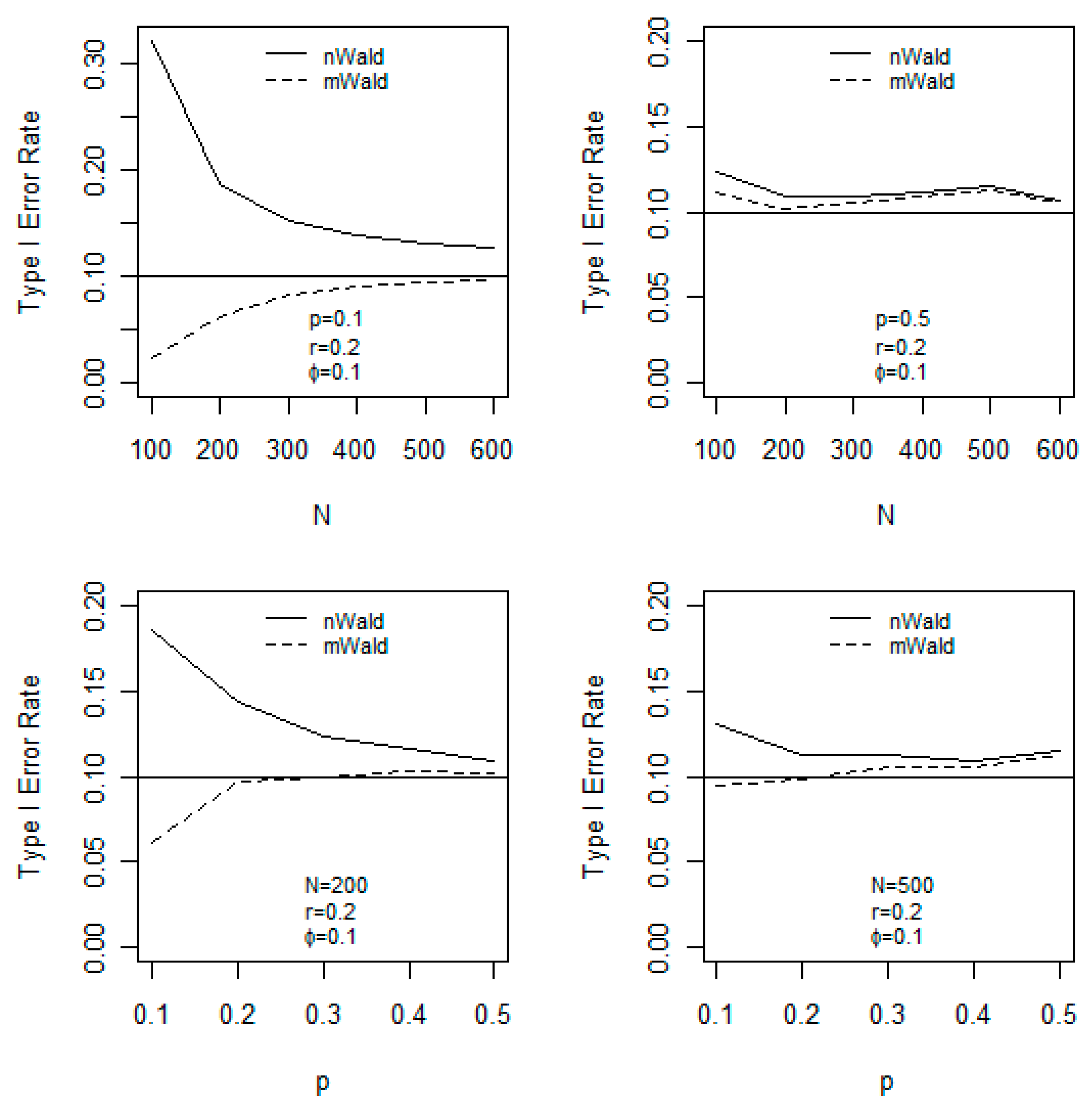
First, the performance of these two tests was investigated in terms of Type-I error rate by differing the total sample sizes. In these simulations, we assumed:

• False positive rate φ = 0.1;
• Ratio of validation sample size versus the total sample size r = n/N = 0.2;
• Total sample sizes N = 100, 200, 300, 400, 500, 600;
• True proportion parameters of interest p = 0.1 and p = 0.5.

The upper two panels in Figure 2 display the graphs of Type I error rate of both tests versus N for p = 0.1 and p = 0.5, respectively. On the upper-left panel (p = 0.1), binomial distributions are skewed; hence are not sufficiently well-behaved (because the distribution is not symmetric but skewed). Hence, in this scenario, the two tests are not anticipated to behave/carry-out well for (relatively) small samples. Nevertheless, the mWald test is conservative (as the graph showed close-to-nominal, in this case, type I error rate of 10% horizontal line) for all sample sizes studied. Both tests have close-to-nominal Type I error rates when the sample size N is greater than 300 (i.e., as the sample size larger than 300, the graph approaches to the nominal/horizontal line, asymptotically). On the contrary, it is well-known that on the upper-right panel (p = 0.5), binomial distributions are quite symmetric around their means and therefore we anticipate both tests to behave/carry-out well in this scenario. It is not surprising that the upper right panel of Figure 2 shows that both tests have close-to-nominal Type I error rates in any case of the sample sizes (i.e., both graphs approach to the nominal level or the horizontal line, in all sample sizes on the graph). The Type I error rate of the mWald test is consistently better than that of the nWald test (because the graphs consistently showed that the mWald have smaller Type I error rates, across all sample size studied).

Second, we examine the performance of the two tests in terms of Type-I error by varying p. In these simulations, the following are assumed:

• False positive rate φ = 0.1;
• Ratio of validation sample size versus the total sample size r = n/N = 0.2;
• Total sample sizes N = 200 and 500;
• True proportion parameters of interest p = 0.1, 0.2, 0.3, 0.4, 0.5.

The lower two panels of Figure 2 graph the Type-I error rate of both tests versus p. On the lower-left panel (N = 200), the graph showed that the mWald test (dashed-line curve) reaches nominal level of the Type-I error rate (which is the horizontal line) when p > 0.2 (as shown on the x-axis), while the nWald test (solid-line curve) attains nominal level of the Type-I error rate when p > 0.4. On the lower-right panel (N = 500), the mWald test reaches nominal level of the Type-I error rate for all p, while the nWald test attains nominal level of the Type-I error rate when p > 0.2. We note that via manually coding [18] using R version 4.1.2 software with the above specified computer machine, it took 2.069883 min to produce the simulations displayed in Figure 2.

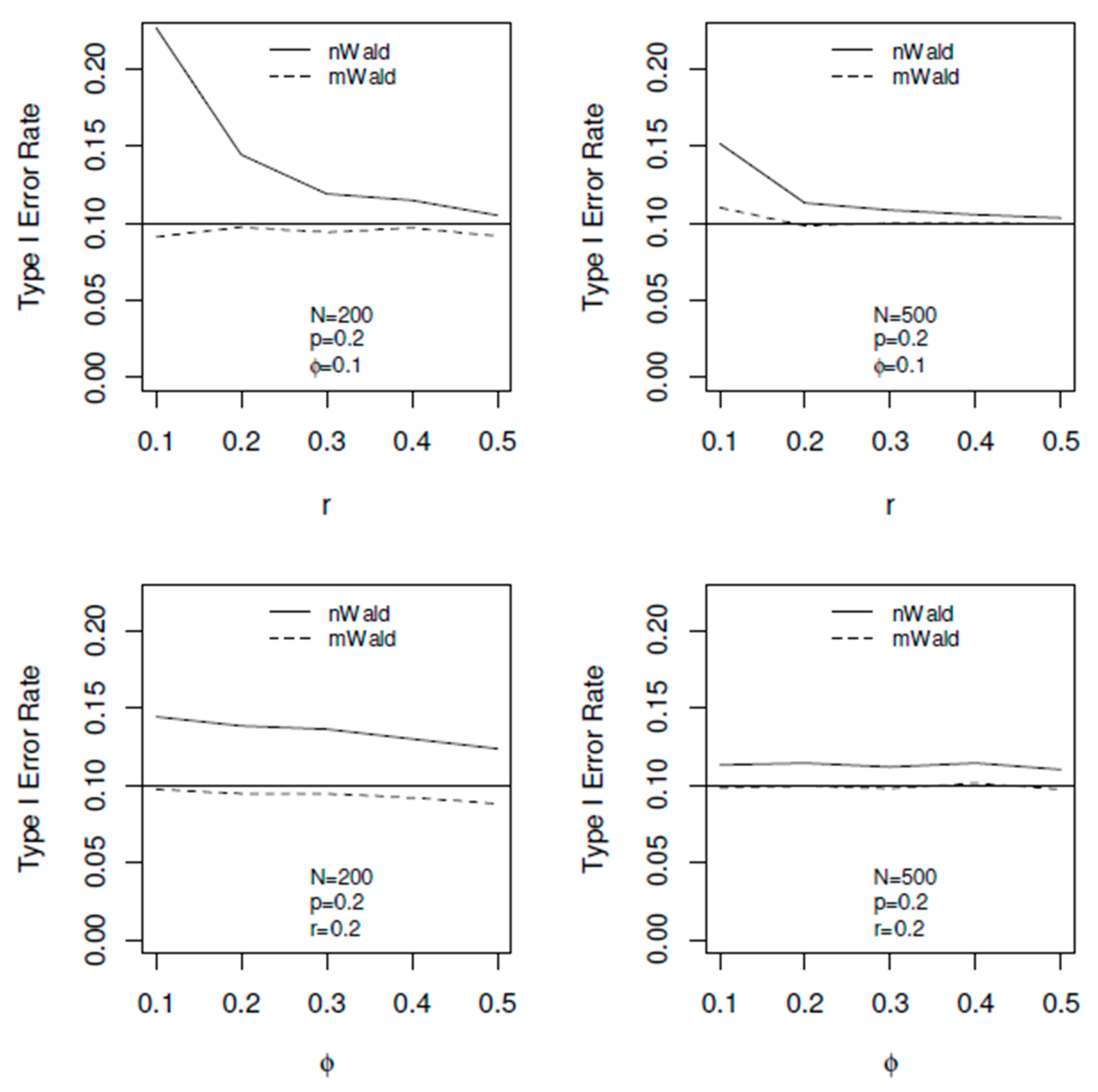
Third, we also evaluate the Type-I error rate of the two tests by varying r. In the simulations, the following are the specifications.

• False positive rate φ = 0.1.
• Ratio of substudy sample size versus the total sample size r = n/N = 0.1, 0.2,…, 0.5.
• Total sample sizes N = 200 and 500.
• True proportion parameters of interest p = 0.2.

In the upper two panels of Figure 3, we graph Type I error rate of both omnibus tests versus r for N = 200 and N = 500, subsequently. When N = 200, the upper left panel of Figure 3 demonstrates that the nWald test (solid-line curve) has inflated Type-I error rates for all r (since the solid-line curve are way above the nominal/horizontal line), especially when r is small. The nWald test has better coverage as r increases. On the contrary, the mWald test has close-to-nominal levels for all the r values studied here (since the dashed-line curve are very close to the horizonal line). Similar observations can be made for N = 500 with both tests having better Type-I error rates.

Forth and finally, we assess the Type-I error rate of the two tests by varying φ. In the simulations, below are the specifications:

• False positive rate φ = 0.1, 0.2, …, 0.5.
• Ratio of substudy sample size versus the total sample size r = n/N = 0.2.
• Total sample sizes N = 200 and 500.
• True proportion parameters of interest p = 0.2.

The lower two panels in Figure 3 graph Type-I error rate of both tests versus φ for N = 200 and 500, respectively. For both N, the lower two panels of Figure 3 demonstrate that the nWald test has inflated Type-I error rates (because the solid-line curve are inflated above the horizontal line), while the mWald test has close-to-nominal levels for all the φ values studied here (because the dashed-line curve almost overlapped the horizontal line). The values of φ do not affect the Type-I error rates for both tests and both N (because both curves are quite flat across all studied values of φ, as shown in the graph). Note that the above computer machine took 1.548624 min using R version 4.1.2 software [18] to run the simulations displayed in Figure 3.

5.2. Power

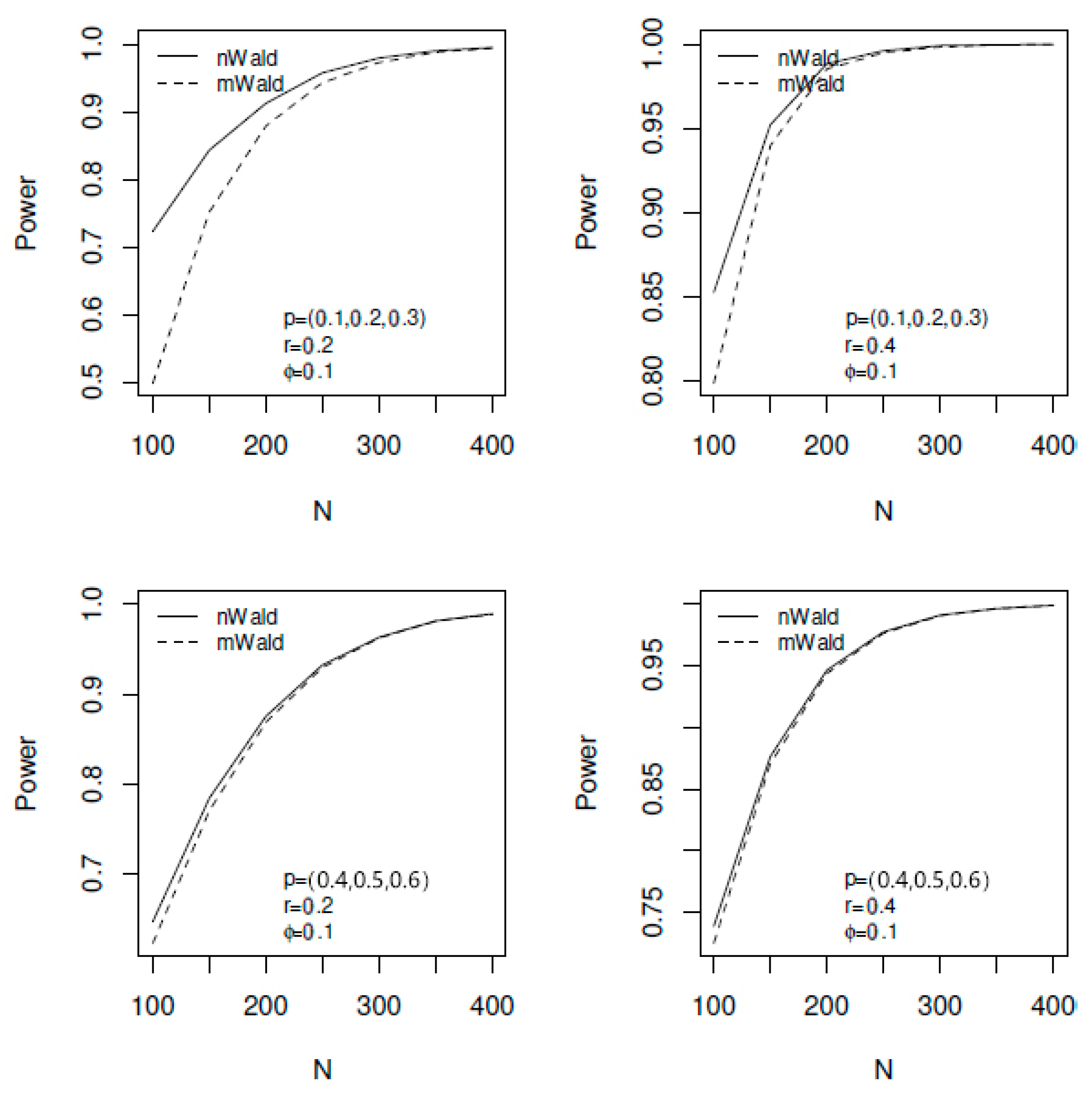
We also examine the power of the two tests. In these simulations, we choose the following.

• False-positive rate φ = 0.1.
• Ratio of substudy sample size versus the total sample size r = n/N = 0.2, 0.4.
• Total sample sizes N = 100, 150, …, 400.
• True proportion parameters of interest p = (0.1, 0.2, 0.3) and p = (0.4, 0.5, 0.6).

The upper two panels of Figure 4 graph the power of both tests versus N for p = (0.1, 0.2, 0.3); the lower two panels graph the power of both tests versus N for p = (0.4, 0.5, 0.6). Note that theoretically, binomial distribution sufficiently well behaved when p close to 0.5 (i.e., “fair-coin” behavior) and not sufficiently well behaved when p is further away from 0.5—this is why we selected such contrasted selections of p = (0.1, 0.2, 0.3) and p = (0.4, 0.5, 0.6). For both sets of p and both r values, the nWald test is uniformly more powerful than the mWald test (as shown on the graph that the solid-line curve uniformly lay above the dashed-line curve), especially when the sample size is small. For larger sample sizes, both tests have similar powers. However, note that when sample size is small, the nWald test inflates the Type-I error rate and, therefore, should be not be used; therefore, the power comparison is not meaningful in these cases. Additionally, note that with the above computer machine specifications, the processing time in R software [18] is 1.904431 min for the simulation results displayed in Figure 4.

6. Summary Discussion, Limitations and Future Research

The summary is as follows. In this manuscript, we considered testing the relationship between a nominal input variable (with multiple levels or groups) and a binomial output variable in doubly sampled framework with under-reported data. We begin with deriving closed-form formulas for the MLE of all the parameters via reparameterization. Subsequently, we constructed two omnibus tests (nWald test and mWald test) by applying the Wald test procedures.

As example to demonstrate the procedures, both tests were applied to the same vehicle-accident dataset used in the Rahardja (2020) paper [1], first introduced by Hochberg in 1977 [17]. Note that to be deemed valid, in general, most statistical methodologies developed and published historically in the bibliography are derived based on the Asymptotic (Large-Sample) Theory. This is why in the standard university-level introductory statistics (Stat 101) course, as the general rule-of-thumb and simplified case, students are taught that large sample was defined as big as 30 samples. Therefore, as anticipated, by Asymptotic (Large-Sample) Theory, the two omnibus tests yielded similar results due to their large-sample size nature of Hochberg (1977) vehicle-accident dataset [17].

Note also that in the case of small sample situations, for examples, in the Biology field, or in a Pilot Study of typical drug developments, where practitioners often encounter small sample, then the results should be noted with precautions. Meaning, if the results from the omnibus test and/or MCP test are not significant, it does not necessarily mean that it is truly not significant; it could be due to insufficient (small) sample size. Such precaution should be included/noted in the labeling or study report. Then, more information needs to be consulted with the subject matter experts (SME) in the field of study, for the final direction of decision making for such small-sample (biology or pilot) study. For example, whether making the decision of “Go/No-Go”; in other words, whether proceeding/not, to next phase (large sample) study, by spending more funds to recruit more patients/sample (with such noted risk or precaution); or terminate the study since it is not promising, etc.

Simulation studies were performed to assess the empirical Type I error rate of both tests under various simulation configurations. Since the two tests were developed based on large-sample theories, both methods were anticipated to implement well under large samples. Such anticipation was affirmed since the resulting Type I error rates were close to the nominal level for large samples. When sample size is relatively small and p is close to 0 or 1, the nWald test resulted in a lot more inflated Type I error rate while the mWald test preserved the Type I error rate. Hence, the mWald test is recommended over nWald test.

The limitations are as follows. When sample size is afforded at relatively small size, p is close to 0 or 1, even in larger samples, both methods still suffer from inflation of type I error rate due to: not only asymptotic approximation, but also both tests can be conservative, i.e., slow to reject the null hypothesis (Figure 2). In the standard/built-in statistical software packages such as R, SAS, etc., there is the use of continuity adjustment in chi-square test which is most useful for small sample sizes, to prevent overestimation of statistical significance for small data. The formula is chiefly used when at least one cell of the table has an expected count smaller than five (5). Unfortunately, such correction may tend to overcorrect. This use of the continuity adjustment is somewhat controversial and can result in an overly conservative result that cause the chi-square test fails to reject the null hypothesis when it should (i.e., too conservative), for small sample size.

Finally, in this manuscript, as the first part of a two-stage sequential test (with over-reported data), we have contributed the development of two omnibus tests (first-stage), to test the statistical hypothesis in expression (2), with an easy-to-implement, closed-form algorithm. Indeed, due to our closed-form algorithm via reparameterization, we were able to derive such omnibus tests for g ≥ 3 scenario with the under-report (or WLOG, over-report), which was the reason why previously other researchers were not able to derive such scenario. If such test in expression (2) is not rejected then we declare there is no proportion difference among the g groups. Otherwise, if the test is rejected, then we may want to proceed to the second stage (of the two-stage sequential test) to find-out which pair(s) contributes the difference. In such case, Rahardja pairwise comparison method developed in 2020 [1], which also known as Pairwise Multiple Comparison Procedures (MCP) with over-reported adjustment incorporated via doubly sampled framework, can further be applied. Note also that without incorporating any misclassification (under-reported or over-reported) into the statistical model, such MCP tests are just the standard/classical procedures in the literature review, as prescribed by Hsu in 1996 [19], Edwards and Hsu in 1983 [20], Hsu and Edwards in 1983 [21], and Hsu in 1982 [22]. Moreover, for the future research, one can add multiple covariates (with multiple levels, too) as the input variables, into considerations—in the presence of under-reported or over-reported (output) data. Examples of such multiple-level (input) covariates may be: age category (below 25, 25–40, 40–60, above 60), height category, body-mass-index category, drinking category (never, sometimes, often), etc.

7. Conclusions

In conclusion, we have completed a Two-Stage Sequential Testing development (for multiple binomial proportions using doubly sampled framework with only under-reported or over-reported data). In this manuscript, we derived two Omnibus Tests with the under-reported or over-reported only. Such Omnibus Tests function as the First-Stage of the Two-Stage Sequential Test. Additionally, the Pairwise-MCP Test was already developed by Rahardja in 2020 [1] and function as the Second-Stage of the Two-Stage Sequential Test (with the over-reported or under-reported).