Properties and Limiting Forms of the Multivariate Extended Skew-Normal and Skew-Student Distributions

Abstract

This paper is concerned with the multivariate extended skew-normal [MESN] and multivariate extended skew-Student [MEST] distributions, that is, distributions in which the location parameters of the underlying truncated distributions are not zero. The extra parameter leads to greater variability in the moments and critical values, thus providing greater flexibility for empirical work. It is reported in this paper that various theoretical properties of the extended distributions, notably the limiting forms as the magnitude of the extension parameter, denoted $\tau$ in this paper, increases without limit. In particular, it is shown that as $\tau$, the limiting forms of the MESN and MEST distributions are different. The effect of the difference is exemplified by a study of stockmarket crashes. A second example is a short study of the extent to which the extended skew-normal distribution can be approximated by the skew-Student.

1. Introduction

The skew-normal distribution was introduced in [1] and the skew-Student in [2]. These two distributions share the property that they may be derived formally. There are several methods of derivation of which probably the best known is to consider the bivariate normal distribution of X and Y each with zero mean, unit variance, and correlation $\rho$. The skew-normal distribution then arises by then considering the distribution of X conditional on $Y<0$ [or $Y>0$]. A second method of construction is to consider a random variable $X+\lambda U$ where U has a standard normal distribution truncated from below at zero, written $U\sim TN{\left(0,1;0\right)}^{+}$, where $TN{\left(\mu ,{\sigma }^2;x\right)}^{+}$ denotes a normally distributed variable with mean $\mu$ and standard deviation $\sigma$ truncated from below at x and $\lambda \in \mathbb{R}$. There are similar and equally well-known constructions for the skew-Student and for the multivariate versions of these distributions. That the conditioning variable Y is required to be less than (greater than) zero and that U follows a standard normal distribution truncated from below at zero are, however, limitations. This is for four principal reasons. First, using negative (positive) values of Y to determine whether or not X is observed is self-evidently a limitation. Depending on the application, the appropriate threshold or truncation point for Y might take any nonzero value, as might the value of the mean of its underlying normal distribution. For example, in his recent paper [3] refers to early work by [4]. The latter was concerned with the scores from admission examinations: in such a case, the mean of Y would surely be greater than zero, as would the truncation point. Similarly, there is often no reason a priori for the underlying mean of U to be zero.

Second, empirical evidence reported in the financial economics literature suggests that in the absence of truncation from below at zero, the distribution of the unobserved variable U, denoted $N\left(\tau ,1\right)$ in this paper, exhibits nonzero values of $\tau$ (see, for example, [5] or [6]). In the first method of derivation above, the corresponding conditioning event would that $Y<\tau$ ($Y>\tau$). Such distributions are referred to in the literature (see [7,8]), as extended skew-normal or extended skew-Student. The importance of nonzero values of $\tau$ also arises in stochastic frontier analysis, commonly referred to as SFA. SFA models are used to measure the efficiency of manufacturing companies and organizations such as banks. There is a detailed review of SFA models and methods in [9]. In its basic form, SFA employs linear regression models in which the unobserved residual has two components, commonly written as $ϵ-\nu$. The first term, $ϵ$, is a standard $N\left(0,{\sigma }_{ϵ}^2\right)$ variate. The second term, $\nu$, is a non-negative variate assumed to have an $N\left(0,{\sigma }_{\nu }^2\right)$ distribution, which is truncated from below at zero; that is, a half normal distribution. The expected value of $\nu$, which is nonzero, measures inefficiency. With these assumptions, the residual $ϵ-\nu$ has a skew-normal distribution. A somewhat different model was introduced by [10] in which the half normal variable is replaced one which has an exponential distribution. The paper by [11] shows that under the limit as $\tau \to -\infty$, and with suitable choice of other model parameters, the extended skew-normal distribution encompasses both the half-normal and exponential distributions for the inefficiency term $\nu$. Use of the extended version of the distribution offers greater flexibility in modeling inefficiency: the distribution of the inefficiency variable may exhibit a nonzero mode or may decay steeply.

Nonzero and negative values $\tau$ also arise in the study of stock market crashes. The standard model in financial economics is that returns on risky financial assets follow a multivariate normal distribution. Under this assumption, formally, the basic model of portfolio theory is to consider the conditional distribution of asset returns given a specified return on a market index. The resulting conditional distribution is multivariate normal, leading in essence to regression models for the return on individual assets. In the same manner, a market crash may be studied by considering the distribution of asset returns given that the return on the market index is less than a specified negative value. The resulting distribution is multivariate extended skew-normal. For market crashes, the value of the parameter denoted $\tau$ is both negative and of substantial magnitude. Analogous results arise if it is assumed that returns follow a multivariate Student distribution. In both the normal and Student cases, the distributions that arise as $\tau \to -\infty$ are of interest, one reason being that the limiting properties are different.

Third, use of extended versions of the skew-normal or skew-Student gives greater variability in the moments and critical values of the distributions. For empirical applications, this offers the possibility of better model fit. For some applications, the implied flexibility in the formal foundations may offer insights into the underlying data generation process. Last, in the multivariate case, conditional distributions are always in general of the extended type. Thus, for applications where conditional distributions play a role, extended versions are important if not unavoidable. The formal derivation of a skew-normal regression model as in [5] offers an example of this.

Extended versions of the skew-normal and skew-Student distributions have explicit advantages for some purposes. They offer the potential for greater flexibility in empirical work and, in addition, methodological advantages in some cases. The main aim of this paper is to present properties of the multivariate extended skew-normal (MESN) and multivariate extended skew-Student (MEST) distributions. The results demonstrate the differences from the standard versions. The paper also studies limiting cases of the distributions as the magnitude of the extension parameter $\tau$ increases without limit, extending a result reported in [11]. As the paper shows, these limiting cases are of interest from a theoretical point of view and offer insights for some applications.

The methodological results are illustrated by two applications. First, there is a study of the effect of a stock market crash. The results are different depending on whether the underlying distributions are multivariate normal or Student. The study presented here is theoretical, but its results can inform the development of econometric models of stock returns. Second, some researchers in this area of statistics have suggested informally that the skew-Student could be used as an alternative to the extended skew-normal. For a specified univariate application, it would be straightforward to estimate the parameters of both distributions and then make an informed choice using a test of fit or, for example, consideration of the tails of the distribution. Such an alternative may be attractive, but the suggestion could equally well be made in reverse: the extended skew-normal could be an alternative to the skew-Student. A general investigation of the similarity of the two distributions, particularly for multivariate cases, would be a major task and beyond the scope of this paper. To inform further research into this issue, this paper contains a short study designed to investigate this conjecture.

The structure of this paper is as follows. In Section 2 and Section 3, results for the MESN and MEST distributions, respectively, are presented. The results in these two sections are based on the extended versions of the second method of construction referred to above. Section 4 is concerned with the first method of construction, sometimes referred to in the literature as a hidden truncation model. This section contains the illustrative example of the effect of a stock market crash. The example shows that different behavior arises depending on the choice of model. Section 5 describes a brief investigation into the use of the skew-Student as an alternative to the extended skew-normal. Section 6 offers some concluding remarks. The abbreviations (E)SN and (E)ST are used for the univariate (extended) skew-normal and (extended) skew-Student distributions, respectively, with MSN and MST for the multivariate versions. Examples and graphs are based on univariate distributions, with most numerical results rounded to four decimal places. Notation not defined explicitly in the text is that in common use.

2. Multivariate Extended Skew-Normal Distribution

The multivariate skew-normal distribution was introduced by [12]. The multivariate extended skew-normal distribution, MESN, with an additional parameter, was first described in [13], independently by [8,14]. Following the notation in the third of these papers, the distribution of an n-vector $\mathit{X}$ that follows this distribution is denoted $MES{N}_n(\mathit{\mu },\sum ,\mathit{\lambda },\tau )$. The authors of reference [13] derive the MESN distribution as a hidden truncation model. The authors of reference [8] present a direct derivation and link it to results in [7], who show that conditional distributions are in general of the extended type. The authors of reference [14] derive it as the convolution $\mathit{X}=\mathit{U}+\mathit{\lambda }V$, where the random vector $\mathit{U}$ has the multivariate normal distribution $N_n\left(\mathit{\mu },\sum \right)$ and the scalar random variable V is independently normally distributed as $N\left(\tau ,1\right)$ truncated from below at 0, denoted $V\sim TN{\left(\tau ,1;0\right)}^{+}$. The basic properties of the MESN distribution are described in this section using the notation in [14]. The probability density function of the distribution of $\mathit{X}$ is

$$f_{\mathit{X}}\left(\mathit{x}\right)={\varphi }_n\left(\mathit{x},\mathit{\mu }+\mathit{\lambda }\tau ,\sum +\mathit{\lambda }{\mathit{\lambda }}^T\right)\frac{\mathrm{\Phi }\left\{\tau \omega +{\mathit{\lambda }}^T{\sum }^{-1}\left(\mathit{x}-\mathit{\mu }-\mathit{\lambda }\tau \right)/\omega \right\}}{\mathrm{\Phi }\left(\tau \right)},$$

(1)

where

$$\omega =\sqrt{1+{\mathit{\lambda }}^T{\sum }^{-1}\mathit{\lambda }}.$$

(2)

${\varphi }_n\left(\mathit{x},\mathit{\mu },\sum \right)$ is the probability density function of an n-vector $\mathit{X}$, which has a multivariate normal distribution with mean vector $\mathit{\mu }$ and covariance matrix $\sum$ evaluated at $\mathit{x}$. $\mathrm{\Phi }\left(z\right)$ is the standard normal distribution function evaluated at z, with $\varphi \left(z\right)$ denoting the corresponding density function. The distribution is denoted $\mathit{X}\sim MES{N}_n(\mathit{\mu },\sum ,\mathit{\lambda },\tau )$. The moment generating function of $\mathit{X}$ is

$$M_{\mathit{X}}\left(\mathit{t}\right)=exp\left\{{\left(\mathit{\mu }+\mathit{\lambda }\right)}^T\mathit{t}+{\mathit{t}}^T\left(\sum +\mathit{\lambda }{\mathit{\lambda }}^T\right)\mathit{t}/2\right\}\mathrm{\Phi }\left(\tau +{\mathit{\lambda }}^T\mathit{t}\right)/\mathrm{\Phi }\left(\tau \right).$$

(3)

The mean vector and covariance matrix of the $MESN$ distribution are, respectively

$$E\left(\mathit{X}\right)=\mathit{\mu }+\mathit{\lambda }\left\{\tau +{\xi }_1\left(\tau \right)\right\}=\mathit{\alpha },cov\left(\mathit{X}\right)=\sum +\mathit{\lambda }{\mathit{\lambda }}^T\left\{1+{\xi }_2\left(\tau \right)\right\}=\mathbf{\Omega },$$

(4)

where the function ${\xi }_k\left(z\right)$ is defined as

$${\xi }_k\left(z\right)={\partial }^{k}log\mathrm{\Phi }\left(z\right)/\partial z^k.$$

(5)

Note that the covariance matrix may also be written

$$cov\left(\mathit{X}\right)=\sum +\mathit{\lambda }{\mathit{\lambda }}^T\left\{1-\tau {\xi }_1\left(\tau \right)-{\xi }_1{\left(\tau \right)}^2\right\},$$

(6)

a form that is referred to in Section 3.3. Coskewness and cokurtosis, defined here as the 4th cumulant, are given by

$${\lambda }_i{\lambda }_j{\lambda }_k{\xi }_3\left(\tau \right);{\lambda }_i{\lambda }_j{\lambda }_k{\lambda }_l{\xi }_4\left(\tau \right),$$

(7)

respectively.

For the skew-normal distribution itself, the mean of the underlying truncated normal variable denoted V equals $\sqrt{2/\pi }$. Rounded to four decimal places, this value is shown in panel 2, column 1 of

Table 1. Moments of the truncated normal distribution.

Panel 1: Min
	$\left|\tau \right|\le 1$	$\left|\tau \right|\le 5$	$\left|\tau \right|\le 30$
mean	0.5251	0.1865	0.0333
variance	0.1991	0.0327	0.0011
skewness	0.1169	0.0000	0.0000
kurtosis	0.1981	0.0083	0.0000
kappa4	0.0005	−0.1879	−0.1879
standardized-skewness	0.5918	0.0000	0.0000
standardized-kurtosis	3.0014	2.7609	2.7609
Panel 2: SN
	$\left|\tau \right|\le 1$	$\left|\tau \right|\le 5$	$\left|\tau \right|\le 30$
mean	0.7979	0.7979	0.7979
variance	0.3634	0.3634	0.3634
skewness	0.2180	0.2180	0.2180
kurtosis	0.5109	0.5109	0.5109
kappa4	0.1148	0.1148	0.1148
standardized-skewness	0.9953	0.9953	0.9953
standardized-kurtosis	3.8692	3.8692	3.8692
Panel 3: Max
	$\left|\tau \right|\le 1$	$\left|\tau \right|\le 5$	$\left|\tau \right|\le 30$
mean	1.2876	5.0000	30.0000
variance	0.6297	1.0000	1.0000
skewness	0.2957	0.2957	0.2957
kurtosis	1.1901	2.9998	3.0000
kappa4	0.1148	0.1148	0.1148
standardized-skewness	1.3162	1.8311	1.9935
standardized-kurtosis	4.9974	7.7592	8.9472

Kurtosis is the fourth moment about the mean.

in the row named “mean”. When $\left|\tau \right|\le 1$ the minimum and maximum values of the mean are 0.5251 and 1.2876, respectively, as shown in panels 1 and 3. The corresponding results for the higher moments are shown in in the other rows of column 1 of the table. Columns 2 and 3 shown the analogous results when $\left|\tau \right|\le 5$ and ≤30, respectively. Thus, as well as arising automatically under conditioning, the extended version of the skew-normal provides for more flexibility in the moments of the distribution.

In their Lemma 2, reference [11] report an apparently known result concerning the limiting distribution of $\mathit{X}$ as $\tau \to -\infty$. The lemma is reported here for convenience.

Lemma 1

([11]). Let $\mathit{X}$ be distributed as $MES{N}_n(\mathit{\mu },\sum ,\mathit{\lambda },\tau )$. As $\tau \to -\infty$, the distribution of $\mathit{X}$ tends to the multivariate normal distribution $N_n\left(\mathit{\mu },\sum \right)$.

An implication of this result, described in more detail below, is that as $\tau <0$ increases in magnitude, V has an exponential distribution with parameter $1/\left|\tau \right|$, that is, with mean and standard deviation both equal to $1/\left|\tau \right|$. As $\tau \to \infty$, the distribution of $\mathit{X}$ tends to a multivariate normal with an unbounded mean vector $\mathit{\mu }+\mathit{\lambda }\tau$ but a finite covariance matrix $\sum +\mathit{\lambda }{\mathit{\lambda }}^T$.

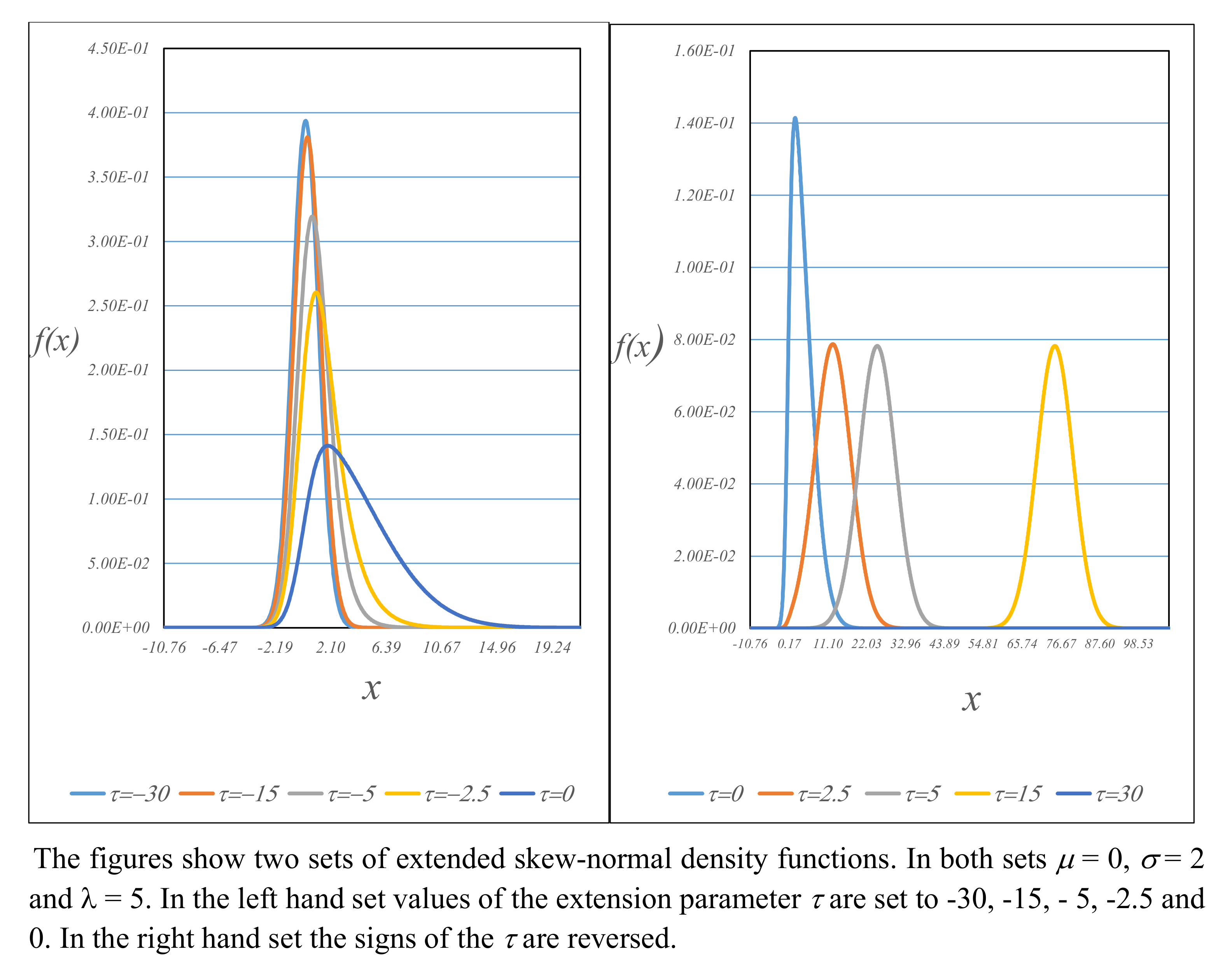
The remainder of this section of the paper presents a number of properties of the MESN distribution. Figure 1 shows two sets of examples of the density function of the (univariate) extended skew-normal distribution for $\tau =\pm 30,\pm 15,\pm 5,\pm 2.5$, and 0. In the left-hand set, the nonzero values of the extension parameter $\tau$ are negative. In the right-hand set, the signs of the $\tau$ are reversed. In both sets, $\mu =0,\sigma =2$, and $\lambda =5$. Both sets demonstrate that asymmetry disappears progressively as $\left|\tau \right|$ increases and exhibit the properties reported in Lemma 1 and the text that follows it.

Papers by [7,15] show that a suitable linear transformation reduces the MSN distribution to a canonical form. Corresponding representations may be derived for the extended version of the distribution and, as shown below, for the extended skew-Student. These representations depend on the following standard result.

Lemma 2.

Let ${\mathit{I}}_{\mathit{n}}$ denote an $n\times n$ unit matrix, $\mathit{\psi }$ an n-vector and ${\mathit{0}}_n$ an n-vector of zeros. The eigenvalues of the matrix ${\mathit{I}}_{\mathit{n}}+\mathit{\psi }{\mathit{\psi }}^T$ are (i) $1+{\mathit{\psi }}^T\mathit{\psi }$ and (ii) 1 repeated $n-1$ times. The corresponding eigenvectors are (i) $\mathit{\psi }/\sqrt{{\mathit{\psi }}^T\mathit{\psi }}$ and (ii) an $n\times \left(n-1\right)$ orthogonal matrix ${\mathit{T}}_0$ which satisfies ${\mathit{\psi }}^T{\mathit{T}}_0={\mathit{0}}_{n-1}^T$.

This is used to establish the following:

Proposition 1.

Let $\mathit{X}\sim MES{N}_n(\mathit{\mu },\sum ,\mathit{\lambda },\tau )$ and let $\mathit{Y}={\sum }^{-1/2}\left(\mathit{X}-\mathit{\mu }\right)$, where ${\sum }^{1/2}$ is a left square-root matrix of Σ. Then, $\mathit{Y}\sim MES{N}_n({\mathit{0}}_n,{\mathit{I}}_n,\mathit{\psi },\tau )$, $\mathit{\psi }={\sum }^{-1/2}\mathit{\lambda }$, and there exists an orthogonal transformation of $\mathit{Y}$

$${\mathit{T}}^T\mathit{Y}={\left(Z_0,{\mathit{Z}}^T\right)}^T,$$

such that $Z_0$ and $\mathit{Z}$ are independently distributed, $Z_0\sim ESN(0,1,\sqrt{{\mathit{\psi }}^T\mathit{\psi }},\tau )$ and $\mathit{Z}\sim N_{n-1}({\mathit{0}}_{n-1},{\mathit{I}}_{n-1})$.

Note that from Lemma 1, as $\tau \to -\infty$, the limiting distribution of $Z_0$ is the standard normal.

2.1. The Truncated Normal Distribution and Its Approximations

The probability density function of the distribution of the truncated normal variable $V\sim TN{\left(\tau ,1;0\right)}^{+}$ is

$$f_V\left(v\right)=\frac{{\varphi }_1\left(v,\tau ,1\right)}{\mathrm{\Phi }\left(\tau \right)}.$$

(8)

The moment-generating function (MGF), originally reported in [16], is

$$M_V\left(t\right)=e^{\tau t+t^2/2}\frac{\mathrm{\Phi }\left(\tau +t\right)}{\mathrm{\Phi }\left(\tau \right)},$$

(9)

with the MGF valid for all $t\in \mathbb{R}$. Following on from [17], numerous authors present results for the moments of the truncated normal distribution and generalizations thereof. These include [18,19,20,21,22] and, recently, [23], among others. For values of $\tau$ that are less than zero, the asymptotic expansion of $\mathrm{\Phi }\left(\tau \right)$ from page 932 of [24] is

$$\varphi \left(\tau \right)\left\{\frac{1}{\left|\tau \right|}+\sum _{j=1}^m\frac{{\left(-1\right)}^j\mathrm{\Gamma }\left(2j\right)}{\mathrm{\Gamma }\left(j\right)2^{j-1}{\left|\tau \right|}^{2j+1}}+R_m\left(\left|\tau \right|\right)\right\}\simeq \varphi \left(\tau \right)\left\{D_m\left(\left|\tau \right|\right)\right\}.$$

(10)

Noting that with suitable choices of m and values of $\tau$, the remainder term $R_m\left(.\right)$

$$R_m\left(\left|\tau \right|\right)=\frac{{\left(-1\right)}^{m+1}\mathrm{\Gamma }\left(2m\right)\left(2m+1\right)}{\mathrm{\Gamma }\left(m\right)2^{m-1}}{\int }_{-\infty }^{\tau }\frac{\varphi \left(x\right)}{x^{2m+1}}dx,$$

(11)

may be ignored. In this case, the moment-generating function of V is

$$M_V\left(t\right)\simeq D_m{\left(\left|\tau \right|\right)}^{-1}\left\{\frac{1}{\left|\tau \right|\left(1-t/\left|\tau \right|\right)}+\sum _{j=1}^m\frac{{\left(-1\right)}^j\mathrm{\Gamma }\left(2j\right)}{\mathrm{\Gamma }\left(j\right)2^{j-1}{\left|\tau \right|}^{2j+1}{\left(1-t/\left|\tau \right|\right)}^{2j+1}}\right\}.$$

(12)

This leads to a distribution for which the corresponding density function is a weighted average of gamma densities

$$f_v\left(v\right)=D_m{\left(\left|\tau \right|\right)}^{-1}\left\{\frac{g\left(v,1/\left|\tau \right|,1\right)}{\left|\tau \right|}+\sum _{j=1}^m\frac{{\left(-1\right)}^j\mathrm{\Gamma }\left(2j\right)g\left(v,1/\left|\tau \right|,2j+1\right)}{\mathrm{\Gamma }\left(j\right)2^{j-1}{\left|\tau \right|}^{2j+1}}\right\},$$

(13)

where $g\left(.\right)$ denotes the density function of the gamma distribution

$$g\left(x,\alpha ,\nu \right)=\frac{x^{\nu -1}{e}^{-x/\alpha }}{{\alpha }^{\nu }\mathrm{\Gamma }\left(\nu \right)};\alpha ,\nu >0.$$

(14)

For sufficiently large values of $\left|\tau \right|$, terms after the first may be ignored, giving an exponential distribution with density function

$$f_V\left(v\right)=\left|\tau \right|e^{-\left|\tau \right|v}.$$

(15)

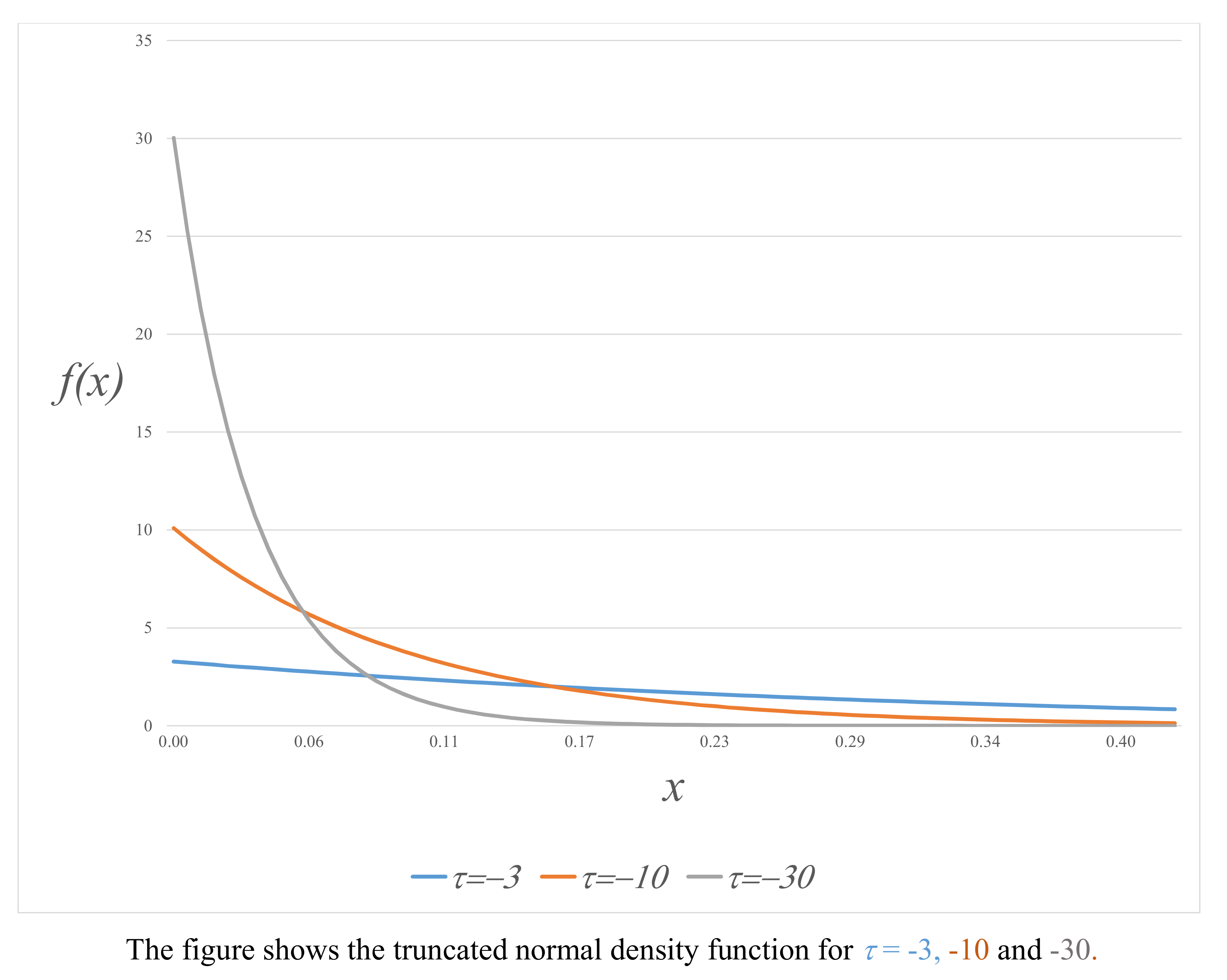
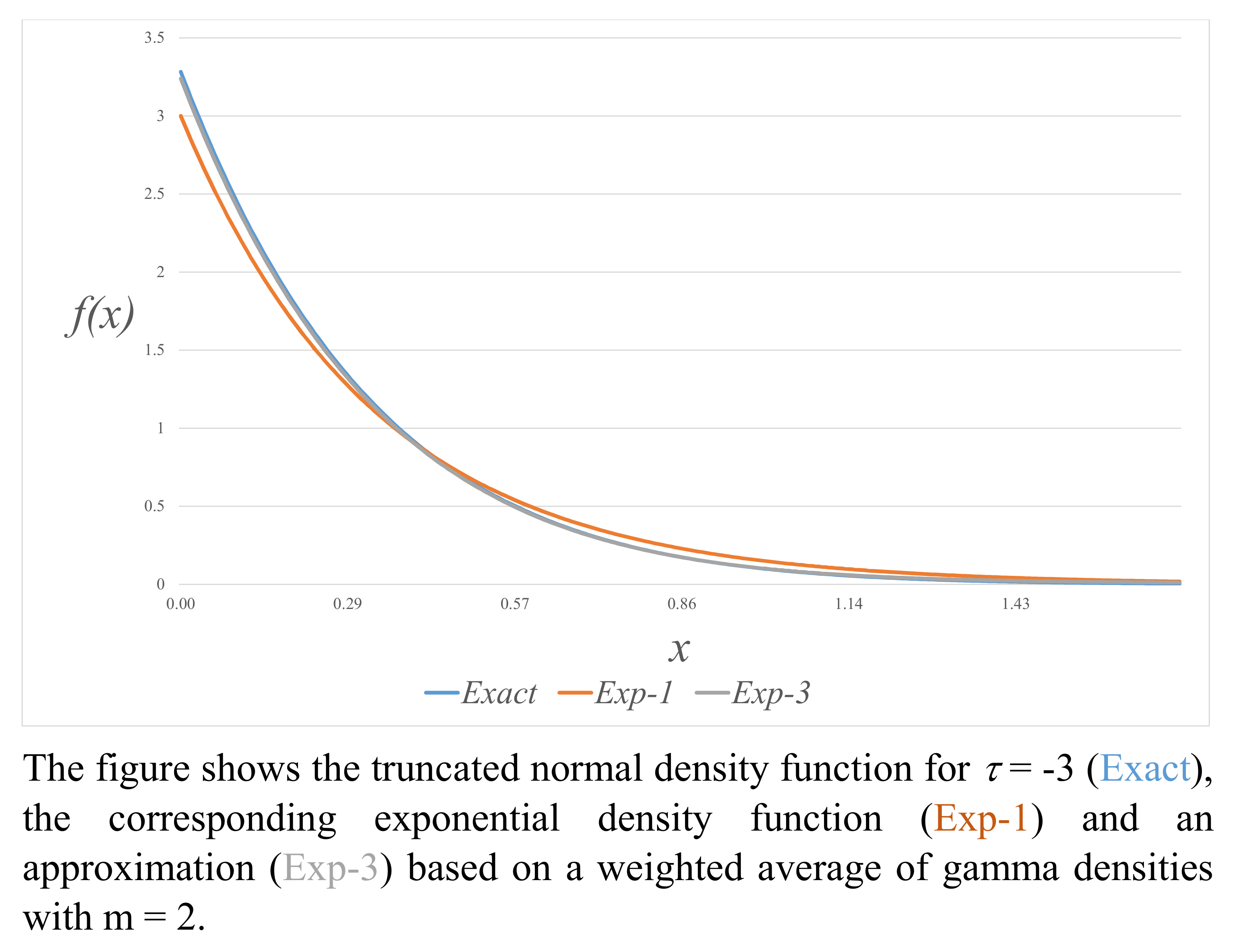
When used to to form the convolution $\mathit{X}=\mathit{U}+\mathit{\lambda }V$, the distribution at (15) leads to the skew-normal exponential distribution described in [11] but originally due to [10]. Figure 2 shows sketches of the truncated normal density function for $\tau =-3,-10$ and $-30$. The steepness of decay increases with $\left|\tau \right|$. Figure 3 shows the truncated normal density function for $\tau =-3$, together with the corresponding exponential density function and and approximation based on the density at Equation (13) with $m=2$. As Figure 3 indicates, the three density functions are visually similar. In particular, there is little difference between the truncated normal density and the three term mixture based on Equation (13).

2.2. Moments of the Truncated Normal Distribution

Expressions for moments of the truncated normal distribution are reported in [21], as well as in references cited above in Section 2.1. In the notation of the present paper, from Equation (9), the mean and variance of the truncated normal distribution are, respectively,

$$E\left(V\right)=\tau +{\xi }_1\left(\tau \right),var\left(V\right)=1+{\xi }_2\left(\tau \right)=1-\tau {\xi }_1\left(\tau \right)-{\xi }_1{\left(\tau \right)}^2={\beta }_1.$$

(16)

Skewness and kurtosis, defined here as the fourth cumulant, are respectively

$${\kappa }_3={\xi }_3\left(\tau \right)={\xi }_1\left(\tau \right)\left\{{\tau }^2-1+3\tau {\xi }_1\left(\tau \right)+2{\xi }_1{\left(\tau \right)}^2\right\}.$$

(17)

and

$${\kappa }_4={\xi }_4\left(\tau \right)={\xi }_1\left(\tau \right)\left(3\tau -{\tau }^3\right)+{\xi }_1{\left(\tau \right)}^2\left(4-7{\tau }^2\right)-12\tau {\xi }_1{\left(\tau \right)}^3-6{\xi }_1{\left(\tau \right)}^4.$$

(18)

Kurtosis, the fourth moment about the mean and denoted by ${\overline{\kappa }}_4$, is

$${\overline{\kappa }}_4={\xi }_4\left(\tau \right)+3{\left\{1+{\xi }_2\left(\tau \right)\right\}}^2.$$

(19)

Expressed in terms of ${\xi }_1\left(\tau \right)$, this is

$${\overline{\kappa }}_4=3-{\xi }_1\left(\tau \right)\left(3\tau +{\tau }^3\right)-{\xi }_1{\left(\tau \right)}^2\left(2+4{\tau }^2\right)-6\tau {\xi }_1{\left(\tau \right)}^3-3{\xi }_1{\left(\tau \right)}^4.$$

(20)

Note that, from [25], ${\kappa }_3\ge 0$ for all $\tau \in \mathbb{R}$. Using the first term of the asymptotic expansion for $\mathrm{\Phi }\left(\tau \right)$ for $\tau \ll 0$, under which V has the exponential distribution at Equation (15), leads to the following expressions for the first four derivatives of $log\mathrm{\Phi }\left(\tau \right)$.

$${\xi }_1\left(\tau \right)\simeq \left|\tau \right|+1/\left|\tau \right|,{\xi }_2\left(\tau \right)\simeq 1/{\tau }^2-1,{\xi }_3\left(\tau \right)\simeq 2/\left|{\tau }^3\right|,{\xi }_4\left(\tau \right)\simeq 6/\left|{\tau }^4\right|,$$

(21)

where in this paper the notation ≃ is taken to mean that the ratio of the two functions tends to unity as, in this case, $\tau \to -\infty$. These results give the same expressions for the first four moments as those computed from the exponential distribution at Equation (15).

Table 2. Moments of the truncated normal distribution and its approximations.

Panel 1: $\mathit{\tau }=-3$
	Exact	Exp-1	Exp-3
mean	0.2831	0.3333	0.2694
variance	0.0706	0.1111	0.0553
skewness	0.0315	0.0741	0.0149
kurtosis	0.0339	0.1111	0.0195
Panel 2: $\mathit{\tau }=-\mathit{10}$
	Exact	Exp-1	Exp-3
mean	0.0981	0.1000	0.0980
variance	0.0094	0.0100	0.0094
skewness	0.0018	0.0020	0.0018
kurtosis	0.0008	0.0009	0.0008
Panel 3: $\mathit{\tau }=-\mathit{30}$
	Exact	Exp-1	Exp-3
mean	0.0333	0.0333	0.0333
variance	0.0011	0.0011	0.0011
skewness	0.0001	0.0001	0.0001
kurtosis	0.0000	0.0000	0.0000

Kurtosis is the fourth moment about the mean. The abbreviations ‘Exact‘, ‘Exp-1‘, and ‘Exp-3‘ are as described in Figure 3.

shows the computed values of the first four moments of the truncated normal distribution, the limiting exponential distribution at Equation (15), and the mixture distribution based on Equation (13) with $m=2$. Values are shown for $\tau =-3,-10$, and $-30$. In the table, kurtosis is the fourth moment about the mean, that is, ${\overline{\kappa }}_4$. As the table shows, the differences between the exact and approximate results are small and decline as $\left|\tau \right|$ increases. Whether a given approximation may be used as a practical alternative to the truncated normal will depend on the magnitude of $\tau$ and the application in question.

2.3. Standardized Form of the Extended Skew-Normal Distribution

Additional insights into the MESN distribution may be obtained by standardization. If ${\mathbf{\Omega }}^{1/2}$ denotes a left square root matrix of $\mathbf{\Omega }$, the random n-vector $\mathit{Z}$ now defined as

$$\mathit{Z}={\mathbf{\Omega }}^{-1/2}\left(\mathit{X}-\mathit{\alpha }\right).$$

(22)

satisfies $E\left(\mathit{Z}\right)={\mathit{0}}_{\mathit{n}}$ and $cov\left(\mathit{Z}\right)={\mathit{I}}_{\mathit{n}}$. The distribution of $\mathit{Z}$ has the density function

$$f_{\mathit{Z}}\left(\mathit{z}\right)={\left|\mathbf{\Omega }\right|}^{1/2}{\varphi }_n\left({\mathbf{\Omega }}^{1/2}\mathit{z},-\mathit{\lambda }{\xi }_1\left(\tau \right),\sum +\mathit{\lambda }{\mathit{\lambda }}^T\right)\frac{\mathrm{\Phi }\left\{{\Delta }_{SSN}\right\}}{\mathrm{\Phi }\left(\tau \right)},$$

(23)

where ${\varphi }_n\left(.\right)$ and $\omega$ are as defined for Equation (1) and

$${\Delta }_{SSN}=\tau \omega +{\mathit{\lambda }}^T{\sum }^{-1}\left({\mathbf{\Omega }}^{1/2}\mathit{z}+\mathit{\lambda }{\xi }_1\left(\tau \right)\right)/\omega .$$

(24)

For the standardized form of extended skew-normal distribution, coskewness and cokurtosis (also defined here in terms of the fourth cumulant) are given by

$${\tilde{\lambda }}_i{\tilde{\lambda }}_j{\tilde{\lambda }}_k{\xi }_3\left(\tau \right);{\tilde{\lambda }}_i{\tilde{\lambda }}_j{\tilde{\lambda }}_k{\tilde{\lambda }}_l{\xi }_4\left(\tau \right),$$

(25)

respectively, where ${\tilde{\lambda }}_i$ is the standardized value of the skewness or shape parameter defined as

$${\tilde{\lambda }}_i=\frac{{\lambda }_i}{{\left[{\sigma }_i^2+{\lambda }_i^2\left\{1+{\xi }_2\left(\tau \right)\right\}\right]}^{1/2}}.$$

(26)

Both coskewness and cokurtosis tend to zero as $\tau \to -\infty$, in which case the limiting distribution of $\mathit{Z}$ is the standard multivariate normal. A suitable transformation similar to that in Proposition 1 shows that the standardized MESN distribution may be expressed in canonical form similar once again to that described in [7] and [15].

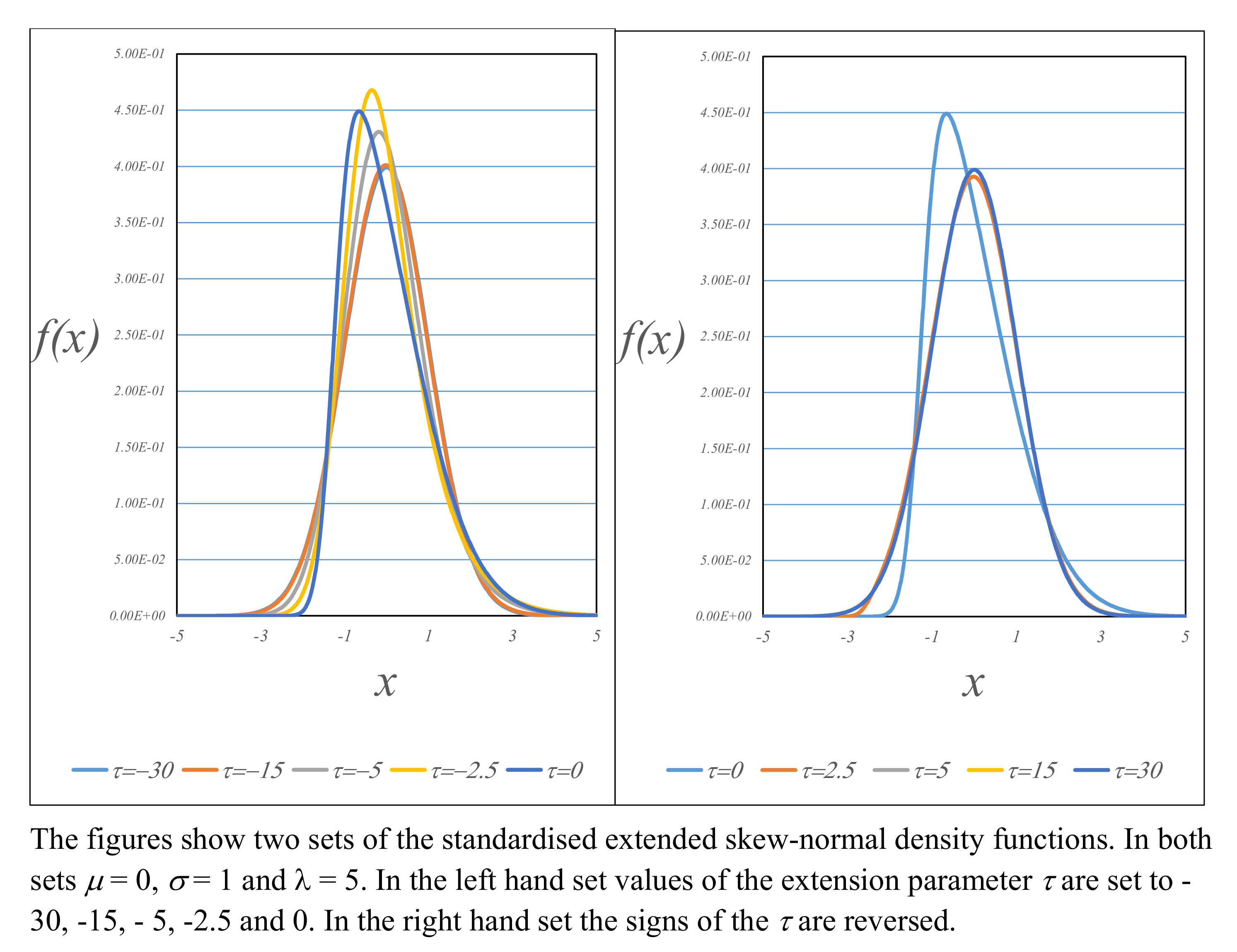
Proposition 2.

Let $\mathit{X}\sim MES{N}_n(\mathit{\mu },\sum ,\mathit{\lambda },\tau )$ and let $\mathit{Y}={\mathbf{\Omega }}^{-1/2}\left(\mathit{X}-\mathit{\alpha }\right)$, where ${\mathbf{\Omega }}^{1/2}$ is a left square-root matrix of Ω and let

$$\mathit{Y}={\left(Y_0,{\tilde{\mathit{Y}}}^T\right)}^T.$$

Then $\tilde{\mathit{Y}}\sim N_{n-1}\left({\mathit{0}}_{n-1},{\mathit{I}}_{n-1}\right)$ and $Y_0\sim ESN\left({\mu }_c,{\sigma }_c^2,{\psi }_c,\tau \right)$ are independently distributed with

$${\mu }_c=-{\psi }_c\left\{\tau +{\xi }_1\left(\tau \right)\right\};{\sigma }_c^2=\frac{1}{\left(1+{\mathit{\psi }}^T\mathit{\psi }{\beta }_1\right)};{\psi }_c=\frac{\sqrt{{\mathit{\psi }}^T\mathit{\psi }}}{\sqrt{\left(1+{\mathit{\psi }}^T\mathit{\psi }{\beta }_1\right)}},$$

and ${\beta }_1$ as defined at Equation (16) and $\mathit{\psi }$ in Proposition 1. Note that as in Proposition 1 as $\tau \to -\infty$ the limiting distribution of $Z_0$ is the standard normal.

Figure 4 shows two sets of standardized extended skew-normal density functions. In both sets $\mu =0$, $\sigma =1$ and $\lambda =5$. In the left-hand set, values of the extension parameter $\tau$ are set to −30, −15, −5, −2.5 and 0. In the right-hand set, the signs of the $\tau$ are reversed. Both sets of densities illustrate that for $\tau \ne 0$ little asymmetry is apparent even when the shape parameter $\lambda$ is substantial; in this case five times greater than the scale parameter $\sigma$. Of the values of $\tau$ shown in the figure, only $\tau =0$ leads to a density function with a discernible amount of asymmetry. 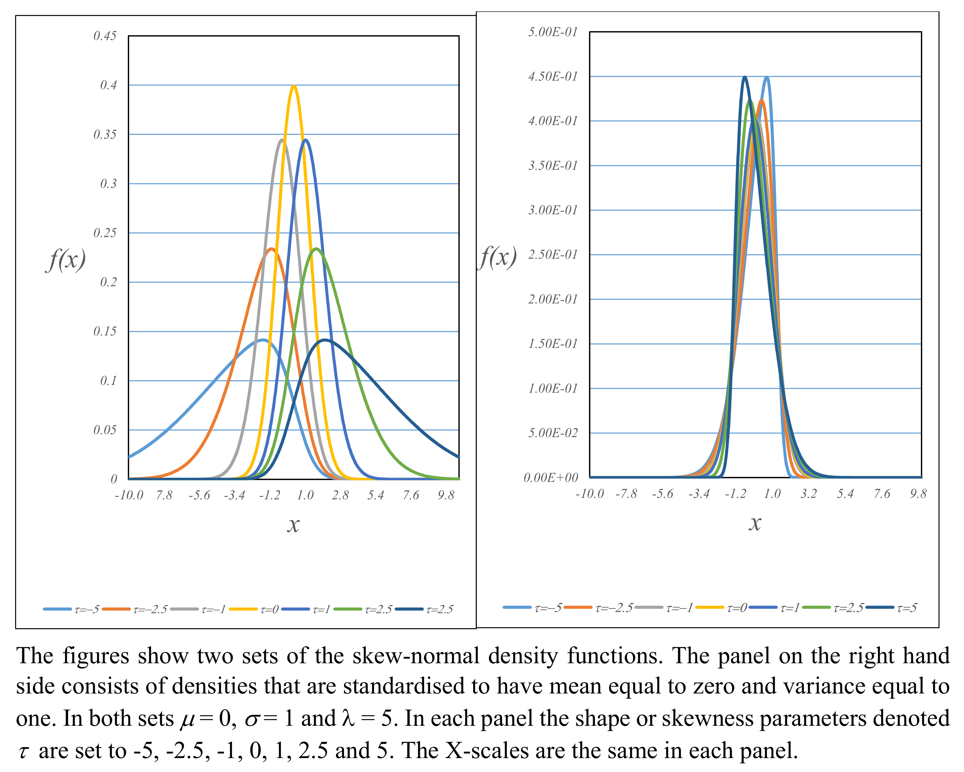Figure 5 shows two more sets of the skew-normal density functions. The panel on the left shows extended skew-normal density functions with $\mu =0,\sigma =1$ and $\lambda =5$. The values of $\tau$ are −5, −2.5, −1, 0, 1, 2.5 and 5. The panel on the right-hand side consists of the corresponding densities standardized to have mean equal to zero and variance equal to one. The X-scales are the same in each panel. As Figure 5 shows, the skewness apparent for the extended skew-normal distributions reduces and largely disappears under standardization. There are analogous results for negative values of $\lambda$.

Table 3. Moments of the extended skew-normal distributions, $\tau \le 0$.

Panel 1: $\mathit{\tau }=0$
	mn	vr	sk	ku	k4	ssk	sku
$\lambda =0$	0.0000	1.0000	0.0000	3.0000	0.0000	0.0000	3.0000
1	0.7979	1.3634	0.2180	5.6912	0.1148	0.1369	3.0617
2.5	1.9947	3.2711	3.4065	36.584	4.4832	0.5758	3.4190
5	3.9894	10.0845	27.2517	376.8234	71.7317	0.8510	3.7053
Panel 2: $\mathit{\tau }=-\mathit{0}.\mathit{5}$
$\lambda =0$	0.0000	1.0000	0.0000	3.0000	0.0000	0.0000	3.0000
1	0.6411	1.2685	0.1626	4.9301	0.1030	0.1138	3.0640
2.5	1.6027	2.6780	2.5407	25.539	4.0239	0.5797	3.5611
5	3.2054	7.7120	20.3255	242.8077	64.3824	0.9491	4.0825
Panel 3: $\mathit{\tau }=-\mathit{1}$
$\lambda =0$	0.0000	1.0000	0.0000	3.0000	0.0000	0.0000	3.0000
1	0.5251	1.1991	0.1169	4.3927	0.0792	0.0891	3.0551
2.5	1.3128	2.2444	1.8270	18.2042	3.0928	0.5434	3.6140
5	2.6257	5.9774	14.6164	156.6738	49.4844	1.0002	4.3850
Panel 4: $\mathit{\tau }=-\mathit{2}.\mathit{5}$
$\lambda =0$	0.0000	1.0000	0.0000	3.0000	0.0000	0.0000	3.0000
1	0.3227	1.0890	0.0429	3.5848	0.0272	0.0377	3.0230
2.5	0.8069	1.5561	0.6700	8.3283	1.0641	0.3452	3.4395
5	1.6137	3.2243	5.3598	48.2146	17.0254	0.9257	4.6376
Panel 5: $\mathit{\tau }=-\mathit{5}$
$\lambda =0$	0.0000	1.0000	0.0000	3.0000	0.0000	0.0000	3.0000
1	0.1865	1.0327	0.0108	3.2045	0.0051	0.0103	3.0048
2.5	0.4663	1.2044	0.1692	4.5501	0.1987	0.1280	3.1370
5	0.9325	1.8174	1.3532	13.0888	3.1799	0.5523	3.9627
Panel 6: $\mathit{\tau }=-\mathit{10}$
$\lambda =0$	0.0000	1.0000	0.0000	3.0000	0.0000	0.0000	3.0000
1	0.0981	1.0094	0.0018	3.0574	0.0005	0.0018	3.0005
2.5	0.2452	1.0590	0.0279	3.3841	0.0194	0.0256	3.0173
5	0.4905	1.2361	0.2233	4.8952	0.3112	0.1625	3.2036
Panel 7: $\mathit{\tau }=-\mathit{20}$
$\lambda =0$	0.0000	1.0000	0.0000	3.0000	0.0000	0.0000	3.0000
1	0.0498	1.0025	0.0002	3.0148	0.0000	0.0002	3.0000
2.5	0.1244	1.0154	0.0038	3.0945	0.0014	0.0037	3.0014
5	0.2488	1.0616	0.0303	3.4032	0.0223	0.0277	3.0198
Panel 8: $\mathit{\tau }=-\mathit{30}$
$\lambda =0$	0.0000	1.0000	0.0000	3.0000	0.0000	0.0000	3.0000
1	0.0333	1.0011	0.0001	3.0066	0.0000	0.0001	3.0000
2.5	0.0831	1.0069	0.0011	3.0418	0.0003	0.0011	3.0003
5	0.1663	1.0276	0.0091	3.1723	0.0045	0.0088	3.0043

Mean, variance, skewness, kurtosis (${\overline{\kappa }}_4$) and 4th cumulant (${\kappa }_4$) are denoted mn, vr, sk, ku & k4 respectively. ssk and sku denote skewness and kurtosis for the standardized distributions.

shows a selection of moments for the extended skew-normal distribution and the corresponding standardized form for values of $\tau$ that are less than or equal to zero. Values of $\tau$ and $\lambda$ are as shown in the table. Values of the location and scale parameter are $\mu =0$ and $\sigma =1$ and are used in all numerical results. As the table shows, when $\tau \le -10$ the values of standardized skewness and kurtosis are numerically close to 0 and 3 respectively, thus supporting the result of Lemma 1. For $\lambda =0$ and 1 there is evidence to support normality for $\tau <-1$. Asymmetry is most evident when $\tau$ is zero or close to it.

Table 4. Moments of the extended skew-normal distributions $\tau \ge 0$.

Panel 1: $\mathit{\tau }=0$
	mn	vr	sk	ku	k4	ssk	sku
$\lambda =0$	0.0000	1.0000	0.0000	3.0000	0.0000	0.0000	3.0000
1	0.7979	1.3634	0.2180	5.6912	0.1148	0.1369	3.0617
2.5	1.9947	3.2711	3.4065	36.584	4.4832	0.5758	3.4190
5	3.9894	10.0845	27.2517	376.8234	71.7317	0.8510	3.7053
Panel 2: $\mathit{\tau }=\mathit{0}.\mathit{5}$
$\lambda =0$	0.0000	1.0000	0.0000	3.0000	0.0000	0.0000	3.0000
1	1.0092	1.4862	0.2710	6.7143	0.0882	0.1496	3.0399
2.5	2.5229	4.0386	4.2342	52.3748	3.4441	0.5217	3.2112
5	5.0458	13.1544	33.8738	574.2185	55.1049	0.7100	3.3185
Panel 3: $\mathit{\tau }=\mathit{1}$
$\lambda =0$	0.0000	1.0000	0.0000	3.0000	0.0000	0.0000	3.0000
1	1.2876	1.6297	0.2957	7.9682	0.0005	0.1421	3.0002
2.5	3.2190	4.9355	4.6206	73.1000	0.0214	0.4214	3.0009
5	6.4380	16.7422	36.9648	841.2418	0.3423	0.5396	3.0012
Panel 4: $\mathit{\tau }=\mathit{2}.\mathit{5}$
$\lambda =0$	0.0000	1.0000	0.0000	3.0000	0.0000	0.0000	3.0000
1	2.5176	1.9556	0.0949	11.3172	−0.1558	0.0347	2.9593
2.5	6.2941	6.9725	1.4835	139.7583	−6.0874	0.0806	2.8748
5	12.5882	24.8899	11.8678	1761.1161	−97.3990	0.0956	2.8428
Panel 5: $\mathit{\tau }=\mathit{5}$
$\lambda =0$	0.0000	1.0000	0.0000	3.0000	0.0000	0.0000	3.0000
1	5.0000	2.0000	0.0000	11.9997	−0.0002	0.0000	3.0000
2.5	12.5000	7.2500	0.0006	157.6791	−0.0064	0.0000	2.9999
5	25.0000	25.9998	0.0045	2027.8688	−0.1022	0.0000	2.9998
Panel 6: $\mathit{\tau }=\mathit{10}$
$\lambda =0$	0.0000	1.0000	0.0000	3.0000	0.0000	0.0000	3.0000
1	10.0000	2.0000	0.0000	12.0000	0.0000	0.0000	3.0000
2.5	25.0000	7.2500	0.0000	157.6875	0.0000	0.0000	3.0000
5	50.0000	26.0000	0.0000	2028.0000	0.0000	0.0000	3.0000
Panel 7: $\mathit{\tau }=\mathit{20}$
$\lambda =0$	0.0000	1.0000	0.0000	3.0000	0.0000	0.0000	3.0000
1	20.0000	2.0000	0.0000	12.0000	0.0000	0.0000	3.0000
2.5	50.0000	7.2500	0.0000	157.6875	0.0000	0.0000	3.0000
5	100.0000	26.0000	0.0000	2028.0000	0.0000	0.0000	3.0000
Panel 8: $\mathit{\tau }=\mathit{30}$
$\lambda =0$	0.0000	1.0000	0.0000	3.0000	0.0000	0.0000	3.0000
1	30.0000	2.0000	0.0000	12.0000	0.0000	0.0000	3.0000
2.5	75.0000	7.2500	0.0000	157.6875	0.0000	0.0000	3.0000
5	150.0000	26.0000	0.0000	2028.0000	0.0000	0.0000	3.0000

Mean, variance, skewness, kurtosis (${\overline{\kappa }}_4$), and fourth cumulant (${\kappa }_4$) are denoted mn, vr, sk, ku, and k4, respectively. ssk and sku denote skewness and kurtosis for the standardized distributions.

shows the corresponding selection for positive values of $\tau$. The panel corresponding to $\tau =0$ is repeated for ease of reading. The table indicates normality for $\tau \ge 5$. Asymmetry is evident when $\tau \le 1$. The panel with $\tau =2.5$ has values of ${\kappa }_4$ that are negative.

3. Multivariate Extended Skew-Student Distribution

The multivariate extended skew-Student distribution, MEST], is an extension of the multivariate skew-Student distribution originally introduced by [2]. The extended version is reported in [26] and later in both [27,28]. Following [14], the former derives it as the convolution $\mathit{X}=\mathit{U}+\mathit{\lambda }V$, where the random vector $\left({\mathit{U}}^T,V\right)$ of length $n+1$ has a multivariate Student distribution with location parameter vector $\left({\mathit{\mu }}^T,\tau \right)$ and scale matrix

$$\begin{array}{c}\hfill \left[\begin{array}{cc}\sum & {\mathit{0}}_n\\ {\mathit{0}}_n^T& 1\end{array}\right],\end{array}$$

(27)

with V truncated from below at zero. Consistent with the notation in Section 1, this is denoted $V\sim T{T}_{\nu }{\left(\tau ,1;0\right)}^{+}$, where $T{T}_{\nu }{\left(\mu ,{\sigma }^2;x\right)}^{+}$ denotes a Student’s t variable with location parameter $\mu$ and scale $\sigma$ truncated from below at x. The marginal distribution of $\mathit{U}$ has the symmetric density function reported Section 3.2 of [27] and independently in [28]. The probability density function of the distribution of $\mathit{X}$ is

$$f_{\mathit{X}}\left(\mathit{x}\right)=t_{\nu ,n}\left(\mathit{x},\mathit{\mu }+\mathit{\lambda }\tau ,\sum +\mathit{\lambda }{\mathit{\lambda }}^T\right)\frac{T_{\nu +n}\left({\Delta }_{ST}\right)}{T_{\nu }\left(\tau \right)},$$

(28)

where

$${\Delta }_{ST}=\frac{\sqrt{\nu +n}\left\{\tau \omega +{\mathit{\lambda }}^T{\sum }^{-1}\left(\mathit{x}-\mathit{\mu }-\mathit{\lambda }\tau \right)/\omega \right\}}{\sqrt{\nu +{\left(\mathit{x}-\mathit{\mu }-\mathit{\lambda }\tau \right)}^T{\left(\sum +\mathit{\lambda }{\mathit{\lambda }}^T\right)}^{-1}\left(\mathit{x}-\mathit{\mu }-\mathit{\lambda }\tau \right)}},$$

(29)

and where $\omega$ is as defined at Equation (2). $t_{\nu ,n}\left(\mathit{x},\mathit{\mu },\sum \right)$ is the probability density function of an n-vector $\mathit{X}$ which has a multivariate Student distribution with location parameter vector $\mathit{\mu }$ and scale matrix $\sum$ evaluated at $\mathit{x}$. $T_{\nu }\left(z\right)$ is the distribution function of a Student’s t variable with $\nu$ degrees of freedom evaluated at z and $t_{\nu }\left(z\right)$ is the corresponding density function. This distribution is denoted $\mathit{X}\sim MES{T}_n(\mathit{\mu },\sum ,\mathit{\lambda },\tau ;\nu )$. As in Section 2, this section of the paper presents basic properties of the MEST distribution. Similar to Table 1, unreported results show that nonzero values of $\tau$ make a substantial difference to the moments of the distribution. As $\tau \to \infty$, the limiting distribution of $\mathit{X}$ is multivariate Student.

Proposition 3.

Let $\mathit{X}\sim MES{T}_n(\mathit{\mu },\sum ,\mathit{\lambda },\tau ;\nu )$. The limiting distribution as $\tau \to \infty$ is multivariate Student with location parameter $\mathit{\mu }+\mathit{\lambda }\tau$, scale matrix $\sum +\mathit{\lambda }{\mathit{\lambda }}^T$, and ν degrees of freedom; denoted $\mathit{X}\sim MV{T}_n(\mathit{\mu }+\mathit{\lambda }\tau ,\sum +\mathit{\lambda }{\mathit{\lambda }}^T;\nu )$.

The proof of this result uses the scale mixture representation reported in Lemma 3 of [29]. This result is consistent with the analogous property of the MESN distribution reported in Section 2. As shown later in this section, however, the limiting distribution of $\mathit{X}$ as $\tau \to -\infty$ in the MEST case is different from that for the MESN.

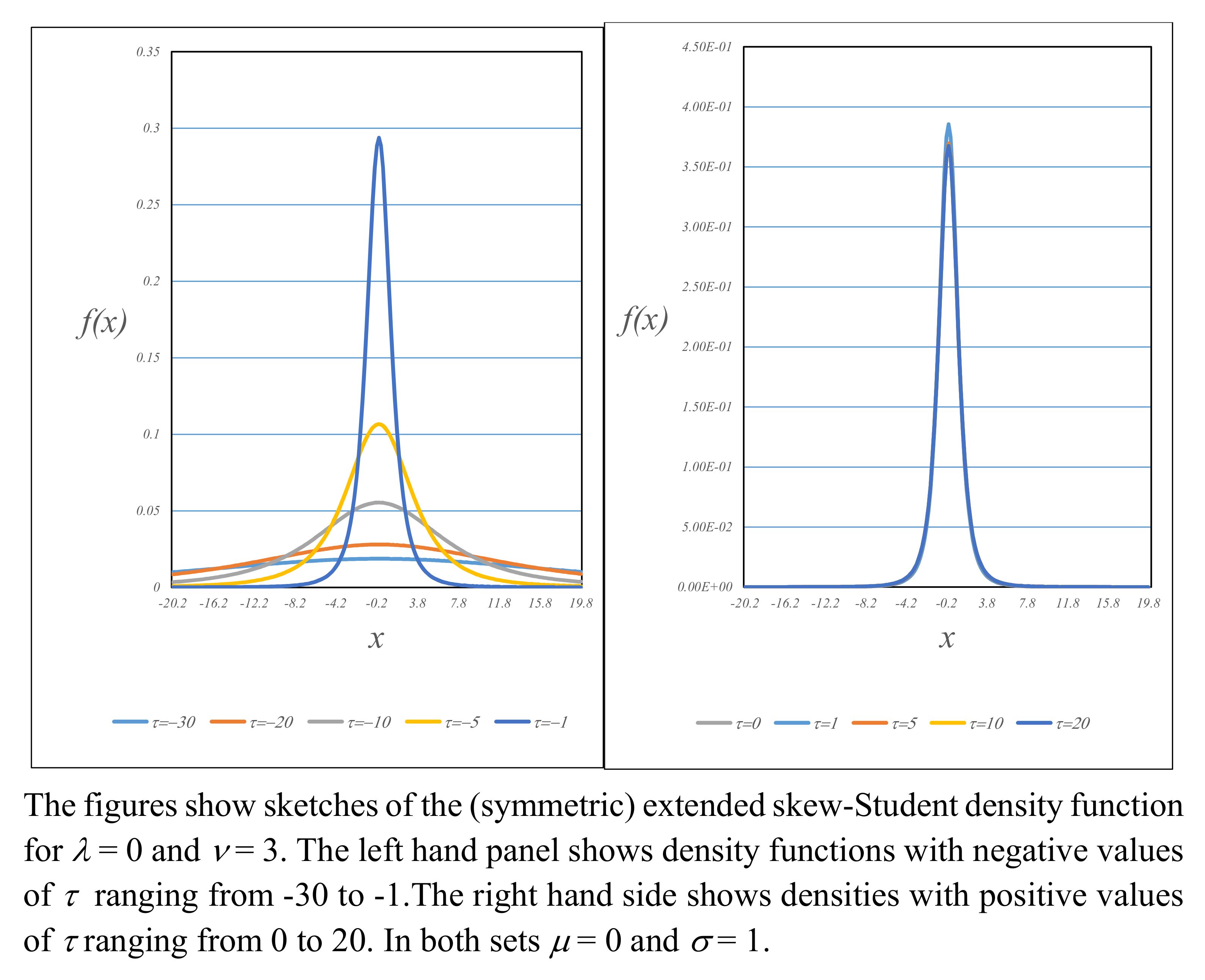
Figure 6 shows sketches of the extended skew-Student density function for $\lambda =0$ and $\nu =3$. The left-hand panel shows density functions with negative values of $\tau$ ranging from $-30$ to $-1$.The right-hand side shows densities with positive values of $\tau$ ranging from 0 to 30. This symmetric density function is that reported in both [27,28]. Two notable features are, first, the similarity of the density function for increasing positive values of $\tau$, but, second, the increasing spread of the density function as $\left|\tau \right|$ increases for negative values of $\tau$. 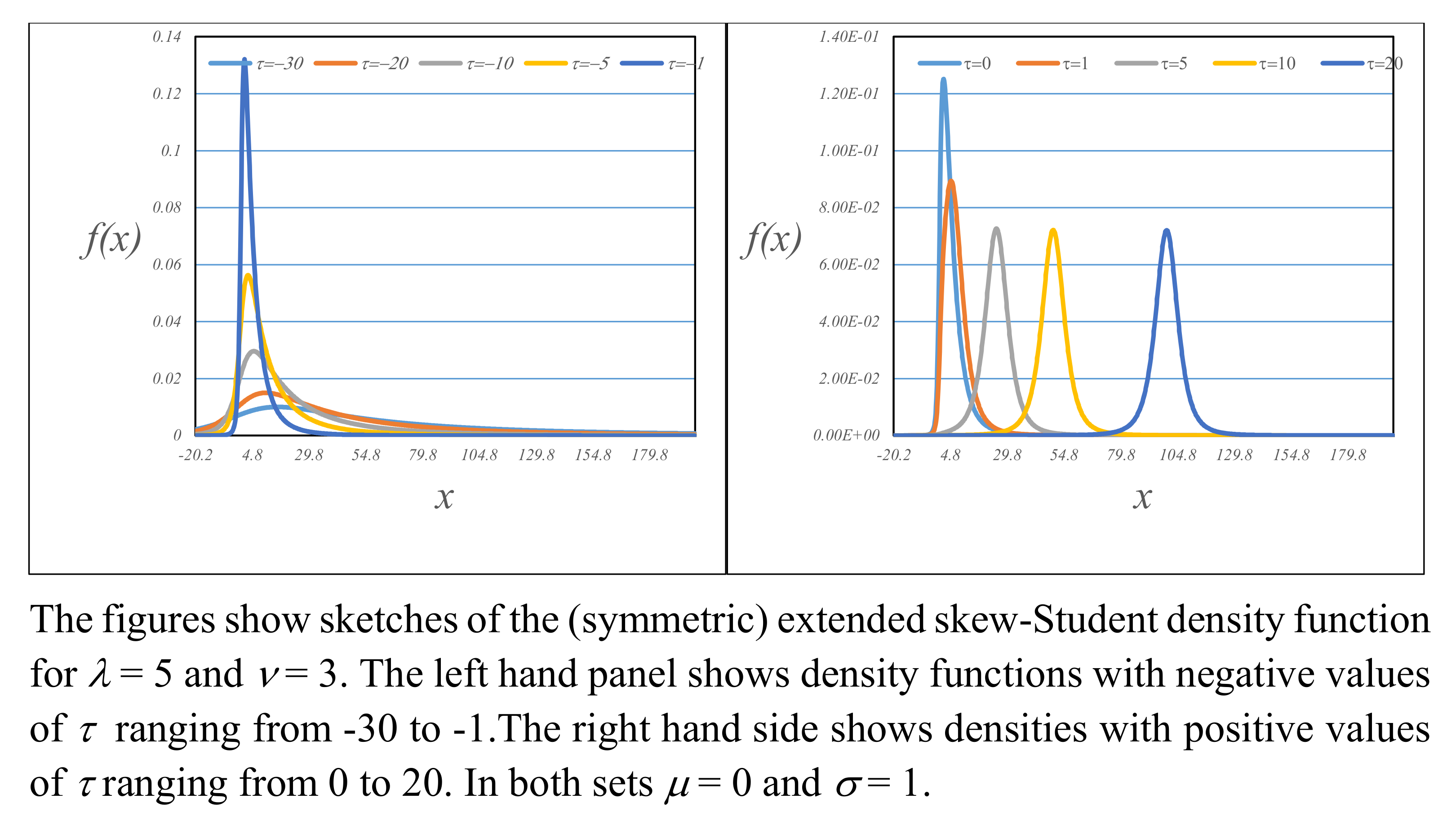For $\lambda =5$, the left-hand panel of Figure 7 shows density functions with the same negative values of $\tau$. The right-hand panel shows densities with $\tau$ ranging from 0 to 20. In both of these figures, $\mu =0$ and $\sigma =1$. In the right-hand panel of Figure 7, the density function is qualitatively similar to the corresponding skew-normal distribution: asymmetry disappears with increasing values of $\tau$, and the location parameter increases, but the spread does not. For negative values of $\tau$, the spread increases and asymmetry decreases with increasing values of $\left|\tau \right|$. To support the sketches in the figures, the moments of the extended skew-Student distribution are reported in Section 3.3 below.

A canonical form of the MEST distribution may be derived using an approach that is essentially the same as that in Proposition 1.

Proposition 4.

Let $\mathit{X}\sim MES{T}_n(\mathit{\mu },\sum ,\mathit{\lambda },\tau ;\nu )$ and let $\mathit{Y}={\sum }^{-1/2}\left(\mathit{X}-\mathit{\mu }\right)$, where ${\sum }^{1/2}$ is a left square-root matrix of Σ. Then $\mathit{Y}\sim MES{T}_n({\mathit{0}}_n,{\mathit{I}}_n,\mathit{\psi },\tau ;\nu )$, $\mathit{\psi }={\sum }^{-1/2}\mathit{\lambda }$, and there exists an orthogonal transformation of $\mathit{Y}$

$${\mathit{T}}^T\mathit{Y}=\tilde{\mathit{Z}}={\left(Z_0,{\mathit{Z}}^T\right)}^T,$$

such that the density function of $\tilde{\mathit{Z}}$ is

$$f\left(z_0,\mathit{z}\right)=\frac{K_{\nu ,n}}{\sqrt{1+{\psi }_0^2}{\left\{1+Q_c\left(\tilde{\mathit{z}}\right)/\nu \right\}}^{(\nu +n)/2}}\frac{T_{\nu +n}\left({\Delta }_{ST,c}\right)}{T_{\nu }\left(\tau \right)};{\psi }_0=\sqrt{{\mathit{\psi }}^T\mathit{\psi }},$$

where $K_{\nu ,n}$ is the normalizing constant for an n-variate multivariate Student distribution with ν degrees of freedom,

$$Q_c\left(\tilde{\mathit{z}}\right)={\mathit{z}}^T{\mathit{z}}^T+\frac{{\left(z_0-{\psi }_0\tau \right)}^2}{\left(1+{\psi }_0^2\right)},$$

and

$${\Delta }_{ST,c}=\frac{\sqrt{\nu +n}\left\{\tau {\omega }_c+{\psi }_0\left(z_0-{\psi }_0\tau \right)/{\omega }_c\right\}}{\sqrt{\nu +Q_c\left(\tilde{\mathit{z}}\right)}};{\omega }_c=\sqrt{1+{\psi }_0^2}.$$

Equivalently, $\tilde{\mathit{Z}}\sim MES{T}_n({\mathit{0}}_n,{\mathit{I}}_n,{\mathit{\psi }}_n,\tau ;\nu )$ where ${\mathit{\psi }}_n={({\psi }_0,{\mathit{0}}_{n-1}^T)}^T$.

Standard manipulations show that $Z_0\sim EST(0,1,{\psi }_0,\tau ;\nu )$ and that the marginal distribution of $\mathit{Z}$ has the symmetric Student-like density function reported in Section 3.2 of [27].

3.1. The Truncated Student’s t Distribution

Similar to the extended skew-normal, the properties of the extended skew-Student distribution are substantially affected by those of the truncated form of Student’s t. The density function of the truncated Student’s t variable v is

$$f_V\left(v\right)=\frac{t_{\nu ,1}\left(v,\tau ,1\right)}{T_{\nu }\left(\tau \right)}.$$

(30)

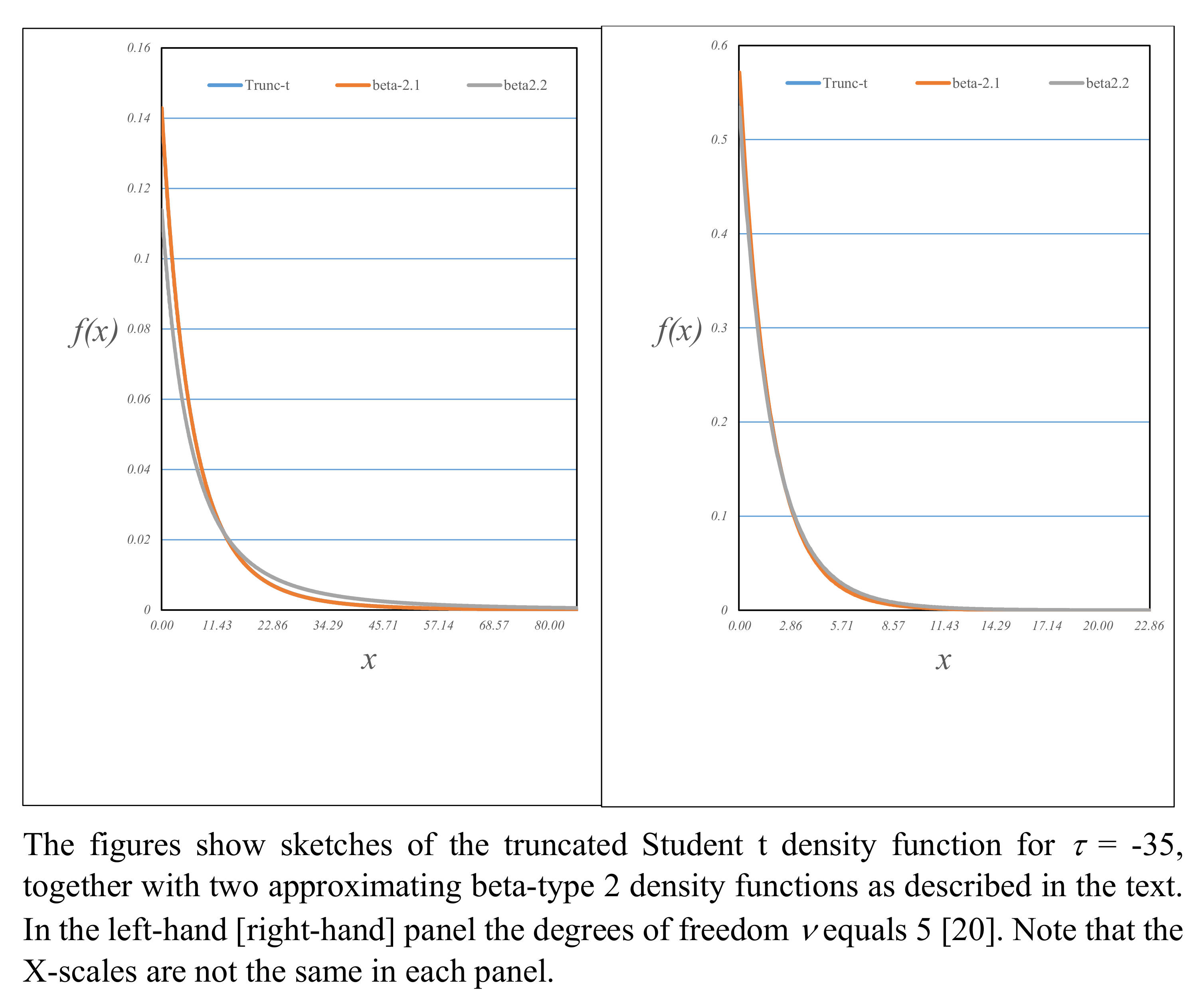
Figure 8 shows sketches of the truncated Student t density function for $\tau =-35$, together with two approximating beta type-2 density functions as described below in Lemma 5. The degrees of freedom $\nu$ are 5 and 20, respectively. For a fixed value of $\tau$, the figure illustrates the increasing severity of decay as $\nu$ increases. It is notable that for $\nu \ge 5$, the truncated Student t is well approximated by the beta type-2 densities.

3.2. Moments of the Truncated Student’s t Distribution

Moments of the truncated distribution at Equation (30) may be evaluated directly. Note that expressions for the moments of a doubly truncated t distribution may be found in [30]. As reported in [27], for $\nu >1$ and $\nu >2$, respectively, the mean and variance of this distribution are

$$E\left(V\right)=\tau +{\xi }_{\nu }\left(\tau \right),var\left(V\right)={\eta }_{\nu }\left(\tau \right)-{\xi }_{\nu }{\left(\tau \right)}^2,$$

(31)

where

$${\xi }_{\nu }\left(\tau \right)=\frac{\nu \left(1+{\tau }^2/\nu \right)t_{\nu }\left(\tau \right)}{\left(\nu -1)T_{\nu }(\tau \right)},{\eta }_{\nu }\left(\tau \right)=-\tau {\xi }_{\nu }\left(\tau \right)+\frac{\nu T_{\nu -2}\left(\tau \sqrt{(\nu -2)/\nu }\right)}{(\nu -2)T_{\nu }\left(\tau \right)}.$$

(32)

The following result, derived using integration by parts, leads to a more useful representation of ${\eta }_{\nu }\left(\tau \right)$.

Lemma 3.

For $\nu >2$, the following result holds

$$\frac{\tau t_{\nu }\left(\tau \right)\left(1+{\tau }^2/\nu \right)}{(\nu -1)T_{\nu }\left(\tau \right)}+\frac{T_{\nu -2}\left(\tau \sqrt{(\nu -2)/\nu }\right)}{T_{\nu }\left(\tau \right)}=1.$$

Using this result, for $\nu >2$, the functions ${\eta }_{\nu }\left(\tau \right)$ and ${\xi }_{\nu }\left(\tau \right)$ are related by the identity

$${\eta }_{\nu }\left(\tau \right)=\frac{\nu }{\nu -2}-\frac{\tau \left(\nu -1\right){\xi }_{\nu }\left(\tau \right)}{\nu -2}.$$

(33)

Equation (33) allows the variance to be written as

$$var\left(V\right)=\frac{\nu }{\nu -2}-\frac{\tau \left(\nu -1\right){\xi }_{\nu }\left(\tau \right)}{\nu -2}-{\xi }_{\nu }{\left(\tau \right)}^2,$$

(34)

Note that $li{m}_{\nu \to \infty }{\xi }_{\nu }\left(\tau \right)={\xi }_1\left(\tau \right)$ is sufficient to show that the limiting values in Equation (31) equal those for the truncated normal at Equation (16). For $\nu >3$ and $\nu >4$, skewess and kurtosis (the fourth moment about the mean), respectively, are

$${\kappa }_3\left(V\right)={\xi }_{\nu }\left(\tau \right)\left\{\frac{\left(\nu -1\right)}{\left(\nu -3\right)}{\tau }^2-\frac{\nu \left(\nu -5\right)}{\left(\nu -2\right)\left(\nu -3\right)}+\frac{3\left(\nu -1\right)}{\left(\nu -2\right)}\tau {\xi }_{\nu }\left(\tau \right)+2{\xi }_{\nu }{\left(\tau \right)}^2\right\}$$

(35)

and

$${\overline{\kappa }}_4\left(V\right)=\frac{3{\nu }^2}{\left(\nu -2\right)\left(\nu -4\right)}+K_1{\xi }_{\nu }\left(\tau \right)+K_2{\xi }_{\nu }{\left(\tau \right)}^2+K_3\tau {\xi }_{\nu }{\left(\tau \right)}^3-3{\xi }_{\nu }{\left(\tau \right)}^4,$$

(36)

where

$$K_1=-\frac{\left(\nu -1\right)}{\left(\nu -4\right)}\left\{{\tau }^3+\frac{3\nu \tau }{\left(\nu -2\right)}\right\};K_2=-\left\{\frac{2\nu \left(\nu +1\right)}{\left(\nu -2\right)\left(\nu -3\right)}+\frac{4\left(\nu -1\right){\tau }^2}{\left(\nu -3\right)}\right\},$$

(37)

and

$$K_3=-\frac{6\left(\nu -1\right)}{\left(\nu -2\right)}.$$

(38)

As already noted above, reference [25] showed that the skewness of the truncated normal distribution is non-negative for all values of $\tau$. The following shows that the same result holds for the truncated Student distribution.

Proposition 5.

Let $V\sim T{T}_{\nu }{\left(\tau ,1;0\right)}^{+}$. For $\nu >3$, the following result holds: ${\kappa }_3\left(V\right)\ge 0$.

The proof is by contradiction. First, note that since ${\xi }_{\nu }\left(\tau \right)\ge 0$, the sign of ${\kappa }_3\left(V\right)$ is determined by the sign of the expression in $\left\{.\right\}$ in Equation (35). This quadratic function of ${\xi }_{\nu }\left(\tau \right)$ has roots

$$\frac{\frac{-3(\nu -1)\tau }{(\nu -2)}}{4}\pm \frac{\sqrt{{\left\{\frac{(\nu -1)\tau }{(\nu -2)}\right\}}^2\left\{\frac{(\nu +1)(\nu -5)}{(\nu -1)(\nu -3)}\right\}+\frac{8\nu (\nu -5)}{(\nu -2)(\nu -3)}}}{4}.$$

Since the coefficient ${\xi }_{\nu }{\left(\tau \right)}^2$ is positive, the function is negative between the roots, which is a contradiction.

Note that as $\nu \to \infty$, Proposition 5 also establishes Sampford’s result, and note that the expressions for the first four moments tend to those for the truncated normal distribution at Equations (16), (17), and (19).

Computation of limiting expressions for the moments as $\tau \to -\infty$ requires a result that is analogous to the well-known asymptotic expression for normal distribution reported in [24]. Such a result was first reported in [31]. As it does not appear to be well known, it is summarized below in the notation of this paper.

Lemma 4

([31]). For values of $\tau$ that are less than zero, the asymptotic expansion of $T_{\nu }\left(\tau \right)$ is

$$t_{\nu }\left(\tau \right)\left(1+{\tau }^2/\nu \right)\left\{\frac{1}{\left|\tau \right|}+\sum _{j=1}^m\frac{{\left(-1\right)}^j\mathrm{\Gamma }\left(2j\right)a_j}{\mathrm{\Gamma }\left(j\right)2^{j-1}{\left|\tau \right|}^{2j+1}}+R_{m,\nu }\left(\left|\tau \right|\right)\right\};a_j=\frac{{\nu }^j\mathrm{\Gamma }\left(\frac{\nu }{2}+1\right)}{2^j\mathrm{\Gamma }\left(\frac{\nu }{2}+1+j\right)}.$$

(39)

Noting that with suitable choices of m and values of $\tau$, the remainder term $R_m\left(.\right)$

$$R_{m,\nu }\left(\left|\tau \right|\right)=\frac{{\left(-1\right)}^{m+1}\mathrm{\Gamma }\left(2m\right)\left(2m+1\right)a_{m+1}}{\mathrm{\Gamma }\left(m\right)2^{m-1}}{\int }_{-\infty }^{\tau }\frac{t_{\nu }\left(x\right)\left(1+{\tau }^2/\nu \right)}{x^{2m+1}}dx,$$

(40)

may be ignored.

Using the first two terms in the expansion in Lemma 4 for $\tau <0$ and $\nu >1$ gives

$${\xi }_{\nu }\left(\tau \right)\simeq \frac{\nu \left|\tau \right|}{\left(\nu -1\right)}+\frac{{\nu }^2}{\left(\nu -1\right)\left(\nu +2\right)\left|\tau \right|}.$$

(41)

from which the asymptotic expected value is

$$E\left(V\right)=\tau +{\xi }_{\nu }\left(\tau \right)\simeq \frac{\left|\tau \right|}{\left(\nu -1\right)}+\frac{{\nu }^2}{\left(\nu -1\right)\left(\nu +2\right)\left|\tau \right|};\tau <0.$$

(42)

For $\nu >2$, the corresponding expression for the asymptotic variance is

$$\frac{{\nu \left|\tau \right|}^2}{{\left(\nu -1\right)}^2\left(\nu -2\right)}+\frac{2\nu \left({\nu }^2-\nu +1\right)}{{\left(\nu -1\right)}^2\left(\nu -2\right)\left(\nu +2\right)}+\frac{{\nu }^3\left({\nu }^3-4{\nu }^2+2\nu -2\right)}{{\left(\nu -1\right)}^2\left(\nu -2\right){\left(\nu +2\right)}^2\left(\nu +4\right){\left|\tau \right|}^2}.$$

(43)

Thus, for fixed finite degrees of freedom $\nu >2$, the expected value and variance increase without limit as $\tau \to -\infty$. As $\nu \to \infty$, the expected value and variance tend to $1/\left|\tau \right|$ and $1/{\left|\tau \right|}^2$, respectively, the results for the truncated normal distribution. The corresponding expressions for skewness and kurtosis are omitted in view of their complexity. However, if just the terms proportional to ${\left|\tau \right|}^3$ are considered, then for $\nu >3$ as $\tau \to -\infty$, asymptotic skewness is

$$\frac{{2\nu \left|\tau \right|}^3}{\left(\nu -1\right)}\left\{\frac{{\nu }^2}{{\left(\nu -1\right)}^2}-\frac{\nu }{\left(\nu -2\right)}+\frac{1}{\left(\nu -2\right)\left(\nu -3\right)}\right\}.$$

(44)

Similarly for $\nu >4$, asymptotic kurtosis is proportional to ${\left|\tau \right|}^4$.

Table 5. Moments of the Truncated Student’s t Distribution.

Panel 1: $\mathit{\tau }=-35$
	mn	vr	sk	ku	k4	ssk	sku
$\nu =5$	8.7755	128.2293	6742.2338	1211054.896	1161726.616	4.6433	73.6528
10	3.9153	19.1388	235.0122	6511.211	5412.3346	2.8069	17.776
100	0.3818	0.1485	0.1177	0.2087	0.1426	2.0568	9.4645
500	0.0986	0.0097	0.0019	0.0009	0.0006	2.0072	9.0581
1000	0.0635	0.004	0.0005	0.0001	0.0001	2.0012	9.0094
Inf	0.0285	0.0008	0.0000	0.0000	0.0000	1.9951	8.9623
Panel 2: $\mathit{\tau }=-\mathit{10}$
$\nu =5$	2.5885	11.0436	168.6874	8789.5951	8423.7139	4.5964	72.0692
10	1.2025	1.7818	6.5701	54.6947	45.1698	2.7623	17.227
100	0.1982	0.0394	0.0157	0.0141	0.0094	2.0083	9.0738
500	0.1180	0.0137	0.0031	0.0016	0.0011	1.9582	8.6753
1000	0.1080	0.0115	0.0024	0.0011	0.0007	1.9521	8.6276
Inf	0.0981	0.0094	0.0018	0.0008	0.0005	1.9460	8.5804
Panel 3: $\mathit{\tau }=-\mathit{1}$
$\nu =5$	0.8144	0.7937	2.4071	24.5591	22.6692	3.4042	38.9844
10	0.6519	0.3797	0.4544	1.3549	0.9224	1.9422	9.3977
100	0.5365	0.2117	0.1328	0.2349	0.1005	1.3628	5.2408
500	0.5274	0.2016	0.1199	0.2049	0.0830	1.3253	5.0441
1000	0.5263	0.2003	0.1184	0.2015	0.0811	1.3208	5.0206
Inf	0.5251	0.1991	0.1169	0.1981	0.0792	1.3162	4.9974
Panel 4: $\mathit{\tau }=\mathit{0}$
$\nu =5$	0.9490	0.7660	1.7094	13.5603	11.7998	2.5496	23.1085
10	0.8647	0.5023	0.5210	1.6356	0.8786	1.4634	6.4821
100	0.8039	0.3741	0.2357	0.5623	0.1424	1.0303	4.0175
500	0.7991	0.3655	0.2214	0.5206	0.1199	1.0021	3.8977
1000	0.7985	0.3644	0.2197	0.5157	0.1173	0.9987	3.8834
Inf	0.7979	0.3634	0.2180	0.5109	0.1148	0.9953	3.8692
Panel 5: $\mathit{\tau }=\mathit{1}$
$\nu =5$	1.4026	0.9677	1.5843	11.8173	9.008	1.6643	12.6197
10	1.3394	0.7530	0.6003	2.4830	0.7821	0.9188	4.3795
100	1.2924	0.6396	0.3153	1.2603	0.0331	0.6163	3.0809
500	1.2885	0.6316	0.2995	1.2035	0.0067	0.5966	3.0167
1000	1.2881	0.6307	0.2976	1.1968	0.0036	0.5942	3.009
Inf	1.2876	0.6297	0.2957	1.1901	0.0005	0.5918	3.0014
Panel 6: $\mathit{\tau }=\mathit{10}$
$\nu =5$	10.0011	1.6523	0.2153	20.4795	12.2891	0.1014	7.5012
10	10.0000	1.2499	0.0011	6.2361	1.5494	0.0008	3.9918
100	10.0000	1.0204	0.0000	3.1888	0.0651	0.0000	3.0625
500	10.0000	1.0040	0.0000	3.0363	0.0122	0.0000	3.0121
1000	10.0000	1.0020	0.0000	3.0181	0.0060	0.0000	3.0060
Inf	10.0000	1.0000	0.0000	3.0000	0.0000	0.0000	3.0000

Mean, variance, skewness, kurtosis (${\overline{\kappa }}_4$), and fourth cumulant (${\kappa }_4$) are denoted mn, vr, sk, ku, and k4, respectively. ssk and sku denote skewness and kurtosis for the standardized distributions.

shows a selection of moments from the truncated Student’s t distribution. As $\tau$ increases above zero, the distribution increasingly resembles Student’s t as demonstrated by the values in the bottom panel of the table. The top panel corresponding to $\tau =-35$ shows the increasing values of the moments. The analog of the limiting exponential distribution that arises in the normal case described in Section 2.1 is as follows.

Lemma 5.

Let $V\sim T{T}_{\nu }{\left(\tilde{\tau },1;0\right)}^{+}$. For $\tau <<0$, as the ratio $\left|\tau \right|/\sqrt{\nu }$ increases without limit, the asymptotic distribution of $Y=V/\left|\tau \right|$ is ${\beta }_{II}\left(1,\nu \right)$, that is, with density function.

$$f_Y\left(y\right)=\frac{\nu }{{\left(1+y\right)}^{\nu +1}}.$$

(45)

The proof of this lemma is in Appendix A. An asymptotically equivalent result is that the variable $\tilde{Y}=V/\sqrt{\nu +{\left|\tau \right|}^2}$ is also distributed as ${\beta }_{II}\left(1,\nu \right)$.

It is straightforward to show that the conditional distribution of $\mathit{X}$ given $V=v$ follows a multivariate Student distribution with $\nu +1$ degrees of freedom, location parameter vector $\mathit{\mu }+\mathit{\lambda }v$, and scale matrix

$$\frac{\nu }{\nu +1}\sum \left\{1+\frac{{\left(v-\tau \right)}^2}{\nu }\right\}.$$

(46)

Use of this distribution in conjunction with the asymptotic distribution of V in Equation (45), for $\tau <0$ does not lead to tractable results that are analogous to those in Section 2.

3.3. Moments of the MEST Distribution

For $\nu >1$ and $\nu >2$, respectively, the mean vector and covariance matrix of the MEST distribution are

$$E\left(\mathit{X}\right)=\mathit{\mu }+\mathit{\lambda }\left\{\tau +{\xi }_{\nu }\left(\tau \right)\right\}={\mathit{\alpha }}_{\nu },$$

(47)

and

$$cov\left(\mathit{X}\right)=\nu \{1+{\eta }_{\nu }\left(\tau \right)/\nu \}\sum /\left(\nu -1\right)+\mathit{\lambda }{\mathit{\lambda }}^T\left\{{\eta }_{\nu }\left(\tau \right)-{\xi }_{\nu }{\left(\tau \right)}^2\right\}={\mathbf{\Omega }}_{\nu }.$$

(48)

Using the identity at Equation (33) allows the covariance matrix to be written as

$$\left\{\frac{\nu }{\left(\nu -2\right)}-\frac{\tau }{\left(\nu -2\right)}{\xi }_{\nu }\left(\tau \right)\right\}\sum +\mathit{\lambda }{\mathit{\lambda }}^T\left\{\frac{\nu }{\left(\nu -2\right)}-\frac{\left(\nu -1\right)}{\left(\nu -2\right)}\tau {\xi }_{\nu }\left(\tau \right)-{\xi }_{\nu }{\left(\tau \right)}^2\right\}.$$

(49)

The similarity of the coeffcient of $\mathit{\lambda }{\mathit{\lambda }}^T$ to the corresponding term in Equation (6) may be noted. The coefficient of $\sum$ provides the inequality $\nu -\tau {\xi }_{\nu }\left(\tau \right)\ge 0$.

The skewness of a single variable $X_i$ in $\mathit{X}$ with scale denoted by $\sigma$ may be expressed in terms of the moments of V the truncated Student’s t variable, specifically Equations (34) and (35), and is given by

$${\kappa }_3\left(X_i\right)=\frac{6{\lambda }_i{\sigma }^2}{\left(\nu -1\right)}var\left(V\right)+{\lambda }_i\left\{{\lambda }_i^2+\frac{3{\sigma }^2}{\left(\nu -1\right)}\right\}{\kappa }_3\left(V\right),$$

(50)

Defining the constants

$$K_4=\frac{3{\nu }^2{\sigma }^4}{\left(\nu -1\right)\left(\nu -3\right)},K_5=\frac{6{\lambda }^2{\sigma }^2\nu }{\left(\nu -1\right)},\chi =\left\{1+\frac{{\xi }_{\nu }{\left(\tau \right)}^2}{\nu }\right\},\vartheta =\left\{1+\frac{3{\xi }_{\nu }{\left(\tau \right)}^2}{\nu }\right\}$$

(51)

The kurtosis of $X_i$ is given by

$$\begin{array}{cc}\hfill {\overline{\kappa }}_4=& K_4{\chi }^2+\left[\frac{2K_4}{\nu }\vartheta +K_5\chi \right]var\left(V\right)+\frac{2{\xi }_{\nu }\left(\tau \right)}{\nu }\left(\frac{2K_4}{\nu }+K_5\right){\kappa }_3\left(V\right)\hfill \\ \hfill & +\left(\frac{K_4+K_5}{\nu }+{\lambda }^4\right){\overline{\kappa }}_4\left(V\right)\hfill \end{array}$$

(52)

The corresponding expressions for coskewness and cokurtosis are omitted. A selection of moments of the extended skew-Student is shown in

Table 6. Extended skew-Student moments, $\mathit{\lambda }=\mathit{0}$, $\mathit{\tau }\le \mathit{0}$.

Panel 1: $\mathit{\tau }=0$
	mn	vr	sk	ku	k4	ssk	sku
$\nu =5$	0.0000	1.6667	0.0000	25.0000	16.6667	0.0000	9.0000
10	0.0000	1.2500	0.0000	6.2500	1.5625	0.0000	4.0000
100	0.0000	1.0204	0.0000	3.1888	0.0651	0.0000	3.0625
1000	0.0000	1.0020	0.0000	3.0181	0.0060	0.0000	3.0060
Panel 2: $\mathit{\tau }=-\mathit{0}.\mathit{5}$
$\nu =5$	0.0000	1.8914	0.0000	33.6814	22.9489	0.0000	9.4148
10	0.0000	1.3270	0.0000	7.0862	1.8033	0.0000	4.0240
100	0.0000	1.0263	0.0000	3.2257	0.0660	0.0000	3.0626
1000	0.0000	1.0026	0.0000	3.0215	0.0061	0.0000	3.0060
Panel 3: $\mathit{\tau }=-\mathit{1}$
$\nu =5$	0.0000	2.2715	0.0000	50.4023	34.9234	0.0000	9.7686
10	0.0000	1.4565	0.0000	8.5803	2.2163	0.0000	4.0448
100	0.0000	1.0361	0.0000	3.2878	0.0673	0.0000	3.0627
1000	0.0000	1.0035	0.0000	3.0273	0.0061	0.0000	3.0060
Panel 4: $\mathit{\tau }=-\mathit{2}.\mathit{5}$
$\nu =5$	0.0000	4.5335	0.0000	184.0710	122.4118	0.0000	8.9559
10	0.0000	2.2167	0.0000	19.9427	5.2015	0.0000	4.0586
100	0.0000	1.0930	0.0000	3.6613	0.0771	0.0000	3.0646
1000	0.0000	1.0091	0.0000	3.0610	0.0063	0.0000	3.0062
Panel 5: $\mathit{\tau }=-\mathit{5}$
$\nu =5$	0.0000	12.3704	0.0000	1630.5664	1171.4828	0.0000	10.6554
10	0.0000	4.8325	0.0000	95.8128	25.7533	0.0000	4.1028
100	0.0000	1.2875	0.0000	5.0778	0.1045	0.0000	3.0631
1000	0.0000	1.0280	0.0000	3.1768	0.0064	0.0000	3.0060
Panel 6: $\mathit{\tau }=-\mathit{10}$
$\nu =5$	0.0000	43.6281	0.0000	20,481.2363	14,770.9983	0.0000	10.7603
10	0.0000	15.2531	0.0000	956.4646	258.4921	0.0000	4.1110
100	0.0000	2.0610	0.0000	13.0118	0.2682	0.0000	3.0631
1000	0.0000	1.1033	0.0000	3.6591	0.0073	0.0000	3.0060
Panel 7: $\mathit{\tau }=-\mathit{20}$
$\nu =5$	0.0000	168.6302	0.0000	306,820.5795	221,512.1022	0.0000	10.7898
10	0.0000	56.9209	0.0000	13,327.5059	3607.5334	0.0000	4.1134
100	0.0000	5.1533	0.0000	81.3467	1.6764	0.0000	3.0631
1000	0.0000	1.4042	0.0000	5.9272	0.0119	0.0000	3.0060

Mean, variance, skewness, kurtosis (${\overline{\kappa }}_4$), and fourth cumulant (${\kappa }_4$) are denoted mn, vr, sk, ku, and k4, respectively. ssk and sku denote skewness and kurtosis for the standardized distributions.

,

Table 7. Extended skew-Student moments, $\mathit{\lambda }=\mathit{0}$, $\mathit{\tau }\ge \mathit{0}$.

Panel 1: $\mathit{\tau }=$ 0
	mn	vr	sk	ku	k4	ssk	sku
$\nu =5$	0.0000	1.6667	0.0000	25	16.6667	0.0000	9.0000
10	0.0000	1.2500	0.0000	6.2500	1.5625	0.0000	4.0000
100	0.0000	1.0204	0.0000	3.1888	0.0651	0.0000	3.0625
1000	0.0000	1.0020	0.0000	3.0181	0.0060	0.0000	3.0060
Panel 2: $\mathit{\tau }=$ 0.5
$\nu =5$	0.0000	1.5613	0.0000	20.9306	13.6175	0.0000	8.5862
10	0.0000	1.2148	0.0000	5.8673	1.4405	0.0000	3.9762
100	0.0000	1.0178	0.0000	3.1723	0.0646	0.0000	3.0624
1000	0.0000	1.0017	0.0000	3.0165	0.006	0.0000	3.0060
Panel 3: $\mathit{\tau }=$ 1
$\nu =5$	0.0000	1.5325	0.0000	19.3630	12.3178	0.0000	8.2452
10	0.0000	1.2076	0.0000	5.7712	1.3965	0.0000	3.9577
100	0.0000	1.0174	0.0000	3.1699	0.0645	0.0000	3.0623
1000	0.0000	1.0017	0.0000	3.0163	0.006	0.0000	3.0060
Panel 4: $\mathit{\tau }=$ 2.5
$\nu =5$	0.0000	1.5864	0.0000	19.0707	11.5210	0.0000	7.5781
10	0.0000	1.2346	0.0000	5.9154	1.3430	0.0000	3.8812
100	0.0000	1.0199	0.0000	3.1808	0.0603	0.0000	3.0580
1000	0.0000	1.0020	0.0000	3.0174	0.0056	0.0000	3.0056
Panel 5: $\mathit{\tau }=$ 5
$\nu =5$	0.0000	1.6447	0.0000	21.698	13.5834	0.0000	8.0218
10	0.0000	1.2490	0.0000	6.2259	1.5456	0.0000	3.9907
100	0.0000	1.0204	0.0000	3.1888	0.0651	0.0000	3.0625
1000	0.0000	1.0020	0.0000	3.0181	0.0060	0.0000	3.0060
Panel 6: $\mathit{\tau }=$ 10
$\nu =5$	0.0000	1.6631	0.0000	23.2514	14.9539	0.0000	8.4066
10	0.0000	1.2500	0.0000	6.2492	1.5618	0.0000	3.9996
100	0.0000	1.0204	0.0000	3.1888	0.0651	0.0000	3.0625
1000	0.0000	1.0020	0.0000	3.0181	0.0060	0.0000	3.0060
Panel 7: $\mathit{\tau }=$ 20
$\nu =5$	0.0000	1.6662	0.0000	24.114	15.7855	0.0000	8.6861
10	0.0000	1.2500	0.0000	6.2500	1.5625	0.0000	4.0000
100	0.0000	1.0204	0.0000	3.1888	0.0651	0.0000	3.0625
1000	0.0000	1.0020	0.0000	3.0181	0.0060	0.0000	3.0060

Mean, variance, skewness, kurtosis (${\overline{\kappa }}_4$), and fourth cumulant (${\kappa }_4$) are denoted mn, vr, sk, ku, and k4, respectively. ssk and sku denote skewness and kurtosis for the standardized distributions.

,

Table 8. Extended skew-Student moments, $\mathit{\lambda }=\mathit{5}$, $\mathit{\tau }\le \mathit{0}$.

Panel 1: $\mathit{\tau }=0$
	mn	vr	sk	ku	k4	ssk	sku
$\nu =5$	4.7451	20.8175	225.8345	8893.0351	7592.9283	2.3776	20.5207
10	4.3234	13.808	67.6648	1136.224	564.2428	1.3188	5.9594
100	4.0197	10.373	29.6176	412.2307	89.4359	0.8865	3.8312
1000	3.9924	10.1127	27.4779	380.1627	73.3625	0.8544	3.7174
Panel 2: $\mathit{\tau }=-\mathit{0}.\mathit{5}$
$\nu =5$	4.2428	20.5686	255.6472	11,315.5682	10,046.3666	2.7405	26.7465
10	3.6615	11.9424	61.6937	1002.0177	574.1549	1.4949	7.0257
100	3.2465	8.0272	22.5251	273.4801	80.1702	0.9904	4.2442
1000	3.2095	7.7427	20.5341	245.6695	65.8204	0.9531	4.0979
Panel 3: $\mathit{\tau }=-\mathit{1}$
$\nu =5$	4.0722	22.1142	315.8725	16,158.4142	14,691.3031	3.0374	33.0413
10	3.2593	10.9491	58.8277	963.236	603.5869	1.6237	8.0348
100	2.6826	6.3294	16.6811	183.5893	63.4062	1.0476	4.5827
1000	2.6313	6.0116	14.8101	159.1484	50.7318	1.0048	4.4038
Panel 4: $\mathit{\tau }=-\mathit{2}.\mathit{5}$
$\nu =5$	4.7013	37.0039	572.3678	40,066.9291	35,959.0737	2.5428	29.2612
10	2.9672	11.7404	64.0527	1183.1857	769.673	1.5923	8.5839
100	1.7351	3.7196	9.2931	91.7766	50.2701	1.2954	6.6334
1000	1.6257	3.2714	7.5897	71.2506	39.1445	1.2827	6.6577
Panel 5: $\mathit{\tau }=-\mathit{5}$
$\nu =5$	7.1113	93.2773	3369.5085	468,082.58	441,980.58	3.7403	53.7985
10	3.6601	20.7462	172.2246	4829.2945	3538.0859	1.8226	11.2204
100	1.1786	2.6214	2.9360	30.3655	9.7500	0.6918	4.4188
1000	0.9569	1.8905	1.4728	14.3196	3.5974	0.5666	4.0065
Panel 6: $\mathit{\tau }=-\mathit{10}$
$\nu =5$	12.9423	319.7115	21,801.33	5,806,861.72	5,500,215	3.8137	56.81
10	6.0126	59.7887	838.1579	41709.0825	30985.0048	1.8130	11.6679
100	0.9912	3.0218	1.9762	34.4648	7.0701	0.3762	3.7743
1000	0.5401	1.3638	0.3004	6.2757	0.6959	0.1886	3.3742
Panel 7: $\mathit{\tau }=-\mathit{20}$
$\nu =5$	25.2227	1225.9337	164,426.37	86,687,913	82,179,173	3.8306	57.6799
10	11.3418	217.1219	5771.12	555,743	414,318	1.8039	11.7887
100	1.2565	6.7553	4.1809	157.0877	20.1859	0.2381	3.4423
1000	0.3486	1.5238	0.0842	7.0835	0.1174	0.0447	3.0506

Mean, variance, skewness, kurtosis (${\overline{\kappa }}_4$), and fourth cumulant (${\kappa }_4$) are denoted mn, vr, sk, ku, and k4, respectively. ssk and sku denote skewness and kurtosis for the standardized distributions. Some large results in the bottom panel are shown to two decimal places only to preserve the formatting.

and

Table 9. Extended skew-Student moments, $\mathit{\lambda }=\mathit{5}$, $\mathit{\tau }\ge \mathit{0}$.

Panel 1: $\mathit{\tau }=0$
	mn	vr	sk	ku	k4	ssk	sku
$\nu =5$	4.7451	20.8175	225.8345	8893.0351	7592.9283	2.3776	20.5207
10	4.3234	13.8080	67.6648	1136.224	564.2428	1.3188	5.9594
100	4.0197	10.3730	29.6176	412.2307	89.4359	0.8865	3.8312
1000	3.9924	10.1127	27.4779	380.1627	73.3625	0.8544	3.7174
Panel 2: $\mathit{\tau }=\mathit{0}.\mathit{5}$
$\nu =5$	5.6607	22.7023	214.9792	7908.2282	6362.0488	1.9874	15.3441
10	5.3196	16.5847	74.6338	1370.39	545.2293	1.1050	4.9823
100	5.0707	13.4268	36.4146	615.2068	74.3678	0.7401	3.4125
1000	5.0483	13.1811	34.1180	578.1129	56.8906	0.7129	3.3274
Panel 3: $\mathit{\tau }=\mathit{1}$
$\nu =5$	7.0132	25.7246	211.2398	7728.9782	5743.7070	1.6190	11.6795
10	6.6970	20.0320	78.5498	1695.5477	491.7080	0.8761	4.2253
100	6.4618	17.0068	39.6479	888.1371	20.4383	0.5653	3.0707
1000	6.4404	16.7681	37.2234	845.719	2.2097	0.5421	3.0079
Panel 4: $\mathit{\tau }=\mathit{2}.\mathit{5}$
$\nu =5$	12.9818	34.9913	193.6584	8374.6553	4701.4769	0.9356	6.8398
10	12.7471	28.9489	65.1275	2496.4765	-17.6434	0.4181	2.9789
100	12.6007	25.2486	25.7804	1552.3035	-360.1776	0.2032	2.4350
1000	12.5894	24.9254	23.3124	1497.7373	-366.0907	0.1873	2.4107
Panel 5: $\mathit{\tau }=\mathit{5}$
$\nu =5$	25.066	41.1056	97.3139	11,095.1977	6026.176	0.3693	6.5665
10	25.0077	32.2824	10.2403	3921.4378	794.9862	0.0558	3.7628
100	25.0000	26.5298	0.3289	2150.2441	38.7529	0.0024	3.0551
1000	25.0000	26.0519	0.0354	2039.6168	3.5148	0.0003	3.0052
Panel 6: $\mathit{\tau }=\mathit{10}$
$\nu =5$	50.0054	42.971	40.1073	13,286.3928	7746.8656	0.1424	7.1954
10	50.0000	32.4975	4.3103	4122.5494	954.2898	0.0233	3.9036
100	50.0000	26.5306	0.3092	2150.8291	39.2089	0.0023	3.0557
1000	50.0000	26.0521	0.0301	2039.7723	3.6359	0.0002	3.0054
Panel 7: $\mathit{\tau }=\mathit{20}$
$\nu =5$	100.0004	43.2846	19.9348	14,666.6315	9045.9524	0.0700	7.8282
10	100.0000	32.5000	4.1682	4131.0685	962.3212	0.02250	3.9111
100	100.0000	26.5306	0.3092	2150.8291	39.2089	0.0023	3.0557
1000	100.0000	26.0521	0.0301	2039.7723	3.6359	0.0002	3.0054

Mean, variance, skewness, kurtosis (${\overline{\kappa }}_4$), and fourth cumulant (${\kappa }_4$) are denoted mn, vr, sk, ku, and k4, respectively. ssk and sku denote skewness and kurtosis for the standardized distributions.

. Table 6 [7] shows results for $\tau \le 0$ [$\tau \ge 0$] for $\lambda =0$. The panel for $\tau =0$ is repeated for convenience and corresponds to Student’s t distribution. The lower panels of Table 6 show the increasing magnitude of variance and kurtosis as $\left|\tau \right|$ increases, even for $\lambda =0$. Table 8 and Table 9 show the corresponding results for $\lambda =5$. Note that in Table 8, some large results are shown to two decimal places only to preserve the formatting.

3.4. Standardized Forms of the MEST Distribution

As in Section 2.3, further insights into the extended skew-Student distribution may be obtained by standardization. If ${\mathbf{\Omega }}_{\nu }^{1/2}$ denotes a left square root matrix of ${\mathbf{\Omega }}_{\nu }$, the random vector $\mathit{Z}$ now defined as

$$\mathit{Z}={\mathbf{\Omega }}_{\nu }^{-1/2}\left(\mathit{X}-{\mathit{\alpha }}_{\nu }\right).$$

(53)

satisfies $E\left(\mathit{Z}\right)={\mathit{0}}_{\mathit{n}}$ and $cov\left(\mathit{Z}\right)={\mathit{I}}_{\mathit{n}}$. The distribution of $\mathit{Z}$ has the density function

$$f_{\mathit{Z}}\left(\mathit{z}\right)={\left|{\mathbf{\Omega }}_{\nu }\right|}^{1/2}{t}_{\nu ,n}\left({\mathbf{\Omega }}_{\nu }^{1/2}\mathit{z},-\mathit{\lambda }{\xi }_{\nu }\left(\tau \right),\sum +\mathit{\lambda }{\mathit{\lambda }}^T\right)\frac{T_{\nu +n}\left({\Delta }_{SST}\right)}{T_{\nu }\left(\tau \right)},$$

(54)

where $t_{\nu ,n}\left(.\right)$ is as defined for Equation (28), $\omega$ is as defined for Equation (1) and

$${\Delta }_{SST}=\frac{\sqrt{\nu +n}\left[\tau \omega +{\mathit{\lambda }}^T{\sum }^{-1}\left\{{\mathbf{\Omega }}_{\nu }^{1/2}\mathit{z}+\mathit{\lambda }{\xi }_{\nu }\left(\tau \right)\right\}/\omega \right]}{\sqrt{\nu +{\left\{{\mathbf{\Omega }}_{\nu }^{1/2}\mathit{z}+\mathit{\lambda }{\xi }_{\nu }\left(\tau \right)\right\}}^T{\left(\sum +\mathit{\lambda }{\mathit{\lambda }}^T\right)}^{-1}\left\{{\mathbf{\Omega }}_{\nu }^{1/2}\mathit{z}+\mathit{\lambda }{\xi }_{\nu }\left(\tau \right)\right\}}},$$

(55)

The distribution at Equation (54) has a canonical form. First, define

$${\beta }_{0,\nu }=\frac{\nu }{\left(\nu -1\right)}\left\{1+\frac{{\eta }_{\nu }\left(\tau \right)}{\nu }\right\};{\beta }_{1,\nu }=\frac{\left\{{\eta }_{\nu }\left(\tau \right)-{\xi }_{\nu }{\left(\tau \right)}^2\right\}}{{\beta }_0},$$

(56)

partition $\mathit{Z}$ into a scalar $Z_0$ and an $\left(n-1\right)$-vector ${\mathit{Z}}_1$ and let $Q\left(\mathit{Z}\right)$ be the quadratic form

$$Q\left(\mathit{z}\right)={\beta }_{0,\nu }{\mathit{z}}_1^T{\mathit{z}}_1+{\tilde{z}}_0^2;{\tilde{z}}_0=\frac{\left\{\sqrt{{\beta }_{0,\nu }}\sqrt{1+{\beta }_{1,\nu }{\psi }_0^2}{z}_0+{\psi }_0{\xi }_{\nu }\left(\tau \right)\right\}}{\sqrt{1+{\psi }_0^2}};{\psi }_0=\sqrt{{\mathit{\psi }}^T\mathit{\psi }},$$

(57)

where $\mathit{\psi }$ is as defined in Proposition 1. Methods similar to those used in that proposition gives the following result.

Proposition 6.

Let $\mathit{X}\sim MES{T}_n(\mathit{\mu },\sum ,\mathit{\lambda },\tau ;\nu )$ and $\mathit{Z}={\mathbf{\Omega }}_{\nu }^{-1/2}\left(\mathit{X}-{\mathit{\alpha }}_{\nu }\right)$, where ${\mathbf{\Omega }}_{\nu }^{1/2}$ is a left square-root matrix of ${\mathbf{\Omega }}_{\nu }$. Then $\mathit{Z}\sim MES{T}_n({\mathit{\mu }}_{c,\nu },{\sum }_{c,\nu },{\mathit{\lambda }}_{c,\nu },\tau ;\nu )$ where

$${\mathit{\mu }}_{c,\nu }=-{\mathit{\lambda }}_{c,\nu }\left\{\tau +{\xi }_{\nu }\left(\tau \right)\right\};{\mathit{\lambda }}_{c,\nu }={\left\{{\lambda }_{\nu },{\mathit{0}}_{n-1}^T\right\}}^T;{\lambda }_{\nu }=\frac{{\psi }_0}{\sqrt{{\beta }_{0,\nu }(1+{\beta }_{1,\nu }{\psi }_0^2)}},$$

and

$$\begin{array}{c}\hfill {\sum }_{c,\nu }=\left[\begin{array}{cc}{\sigma }_{\nu }^2& {\mathit{0}}_{n-1}^T\\ {\mathit{0}}_{n-1}^T& {\mathit{I}}_{n-1}/{\beta }_{0,\nu }\end{array}\right],{\sigma }_{\nu }^2=1/\left\{{\beta }_{0,\nu }(1+{\beta }_{1,\nu }{\psi }_0^2)\right\}.\end{array}$$

The density function of $\mathit{Z}$ is

$$f_{\mathit{Z}}\left(\mathit{z}\right)=\sqrt{\frac{{\beta }_0^n\left(1+{\beta }_1{\psi }_0^2\right)}{\left(1+{\psi }_0^2\right)}}\frac{K_{\nu ,n}}{{\left\{1+\frac{Q\left(\mathit{z}\right)}{\nu }\right\}}^{\left(\nu +n\right)/2}}\frac{T_{\nu +n}\left({\Delta }_{CSST}\right)}{T_{\nu }\left(\tau \right)},$$

(58)

where

$${\Delta }_{CSST}=\frac{\sqrt{\nu +n}\left(\tau \sqrt{1+{\mathit{\psi }}^T\mathit{\psi }}+\sqrt{{\mathit{\psi }}^T\mathit{\psi }}{\tilde{z}}_0\right)}{\sqrt{\nu +Q\left(\mathit{z}\right)}}.$$

(59)

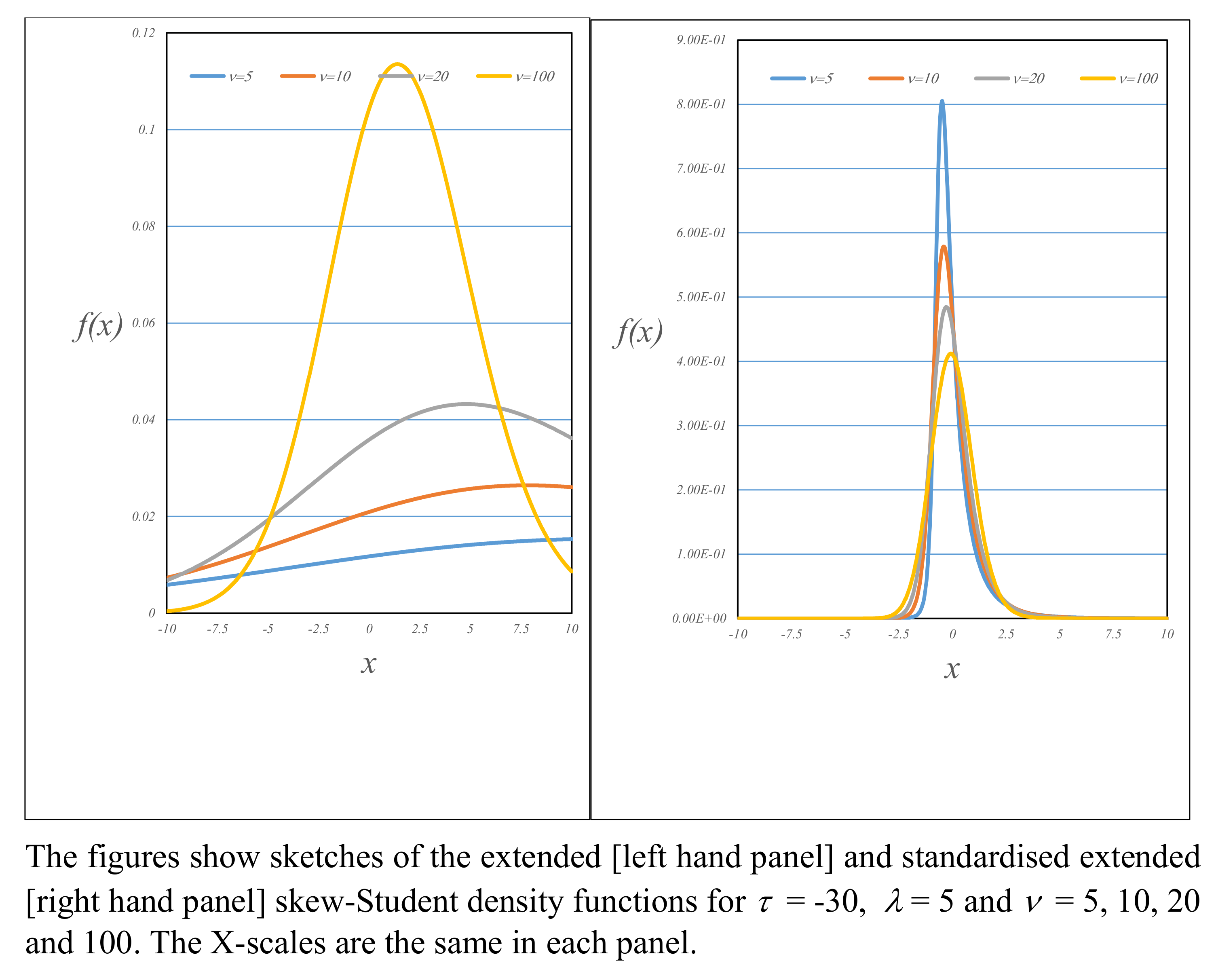
As Equations (58) and (59) show, under the canonical representation, the asymmetry in the density function is attributable solely to the scalar variable ${\tilde{Z}}_0$. The marginal distribution of ${\mathit{Z}}_1$ is symmetric and of the same type reported Section 3.2 of [27]. Examples of the EST and standardized EST density functions are shown in Figure 9 for $\tau =-30$ and $-5$ and $\nu =10,20$, and 100. In the upper (lower) row, $\lambda =0\left[5\right]$. The X-scales are the same in each panel. 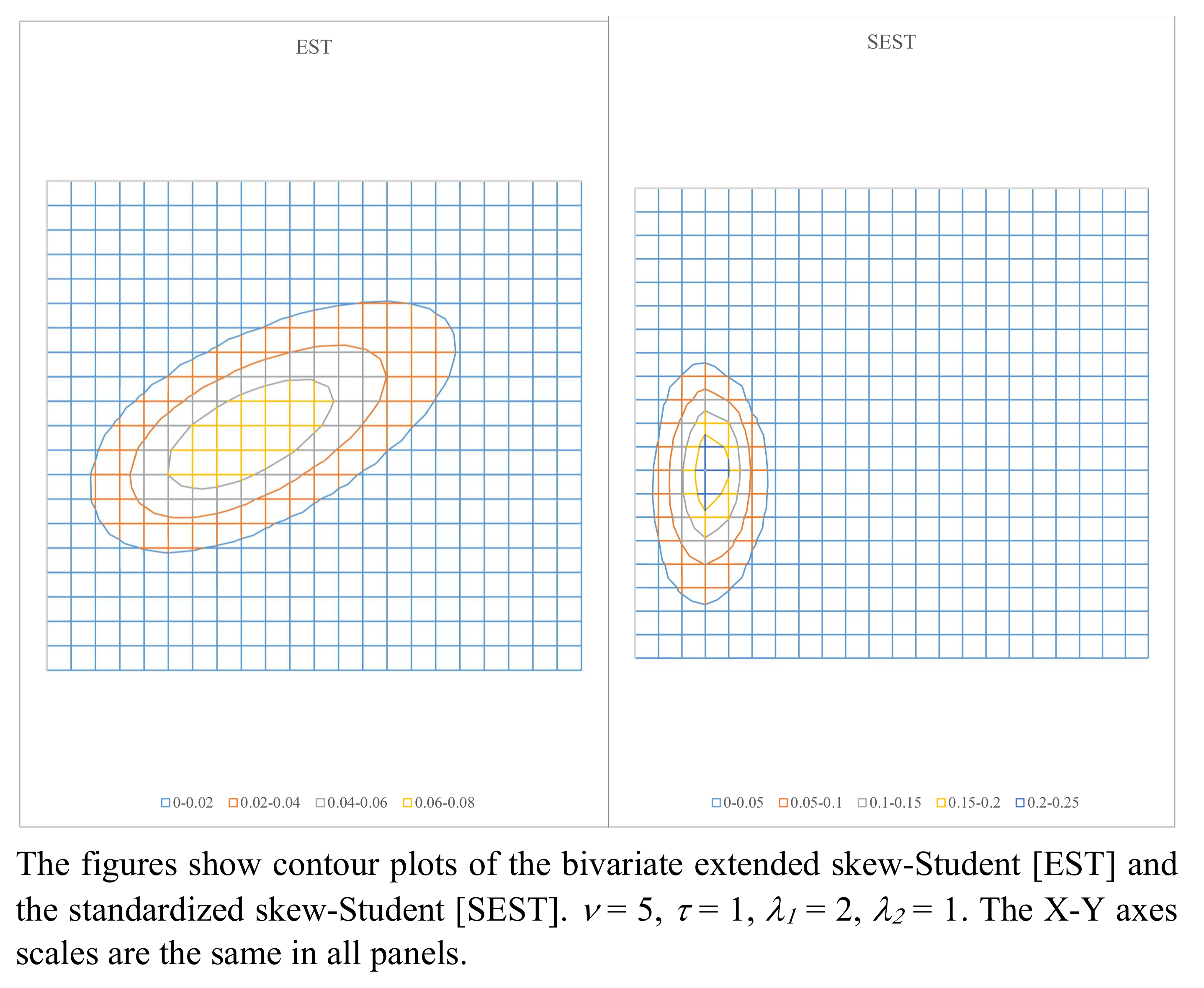The graphs confirm results from Table 8 and Table 09, namely that the degree of asymmetry is reduced under standardization. Examples of contour plots for the bivariate EST and standardized EST distributions are shown in Figure 10.

To investigate the behavior of the distribution as $\tau \to -\infty$ for fixed $\nu$, consider the scalar variable $Z_0$, which has the marginal distribution $EST\left({\mu }_{\nu },{\sigma }_{\nu }^2,{\lambda }_{\nu },\tau ;\nu \right)$ where ${\mu }_{\nu }=-{\lambda }_{\nu }\left\{\tau +{\xi }_{\nu }\left(\tau \right)\right\}$. For $\nu >2$, define

$$A=\frac{\sqrt{\nu (\nu -2)}{\psi }_0}{\sqrt{\nu -1+{\psi }_0^2}};B=\frac{\nu \left\{1+{\psi }_0^2/(\nu -1)\right\}}{(\nu -1)(\nu -2)(1+{\psi }_0^2)}.$$

(60)

As $\tau \to -\infty$ for fixed $\nu$, the asymptotic density function of $Z_0$ is

$$f\left(z_0\right)=\frac{\left|\tau \right|\sqrt{B}{K}_{\nu ,1}}{{\left\{1+{\left(z_0+A\right)}^2{\left|\tau \right|}^{2}B/\nu \right\}}^{(\nu +1)/2}}\frac{T_{\nu +1}\left({\Delta }_{EST}\right)}{T_{\nu }\left(\tau \right)},$$

(61)

where

$${\Delta }_{EST}=\sqrt{\frac{\nu +1}{\nu }}\frac{\left\{\tau \sqrt{1+{\psi }_0^2}+{\psi }_0\left(z_0+A\right)\left|\tau \right|\sqrt{B}\right\}}{\sqrt{1+{\left(z_0+A\right)}^2{\left|\tau \right|}^{2}B/\nu }}.$$

(62)

This leads to the following result:

Proposition 7.

For $\nu >2$, as $\tau /\sqrt{\nu }\to -\infty$, the distribution of $Z_0$ has the asymptotic density function

$$f\left(z_0\right)=\frac{\nu }{B^{\nu /2}{|z_0+A|}^{\nu +1}}{T}_{\nu +1}\left\{\sqrt{\nu +1}\left(\pm {\psi }_0-\frac{\sqrt{1+{\psi }_0^2}}{B^{1/2}|z_0+A|}\right)\right\};z_0\ne -A,$$

(63)

with the sign of ${\psi }_0$ determined by the sign of $z_0+A$, and

$$f\left(-A\right)=\frac{\sqrt{1+{\psi }_0^2}{\nu }^{3/2}{K}_{\nu +1,1}}{{\left(1+{\psi }_0^2\right)}^{\nu /2+1}\sqrt{(\nu -1)(\nu -2)(\nu +1)}}.$$

(64)

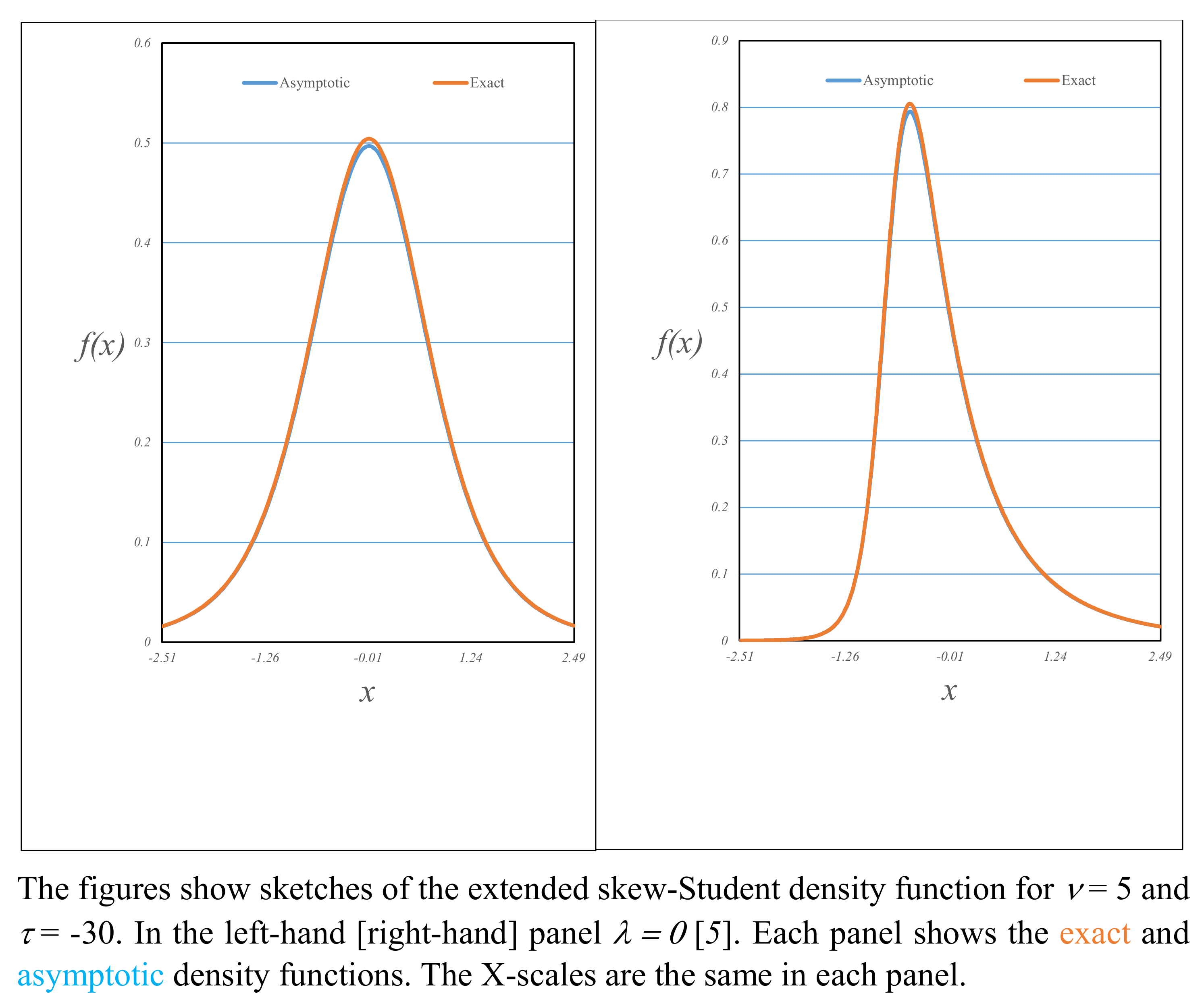
The result in this proposition requires the asymptotic expression for the distribution function of Student’s t. As noted above, such a result was first provided by [31] and is summarized in Lemma 4. Comparative examples of the exact and asymptotic EST density functions are shown in Figure 11. The implication of Proposition 7 is that as $\tau \to -\infty$, the standardized distribution is qualitatively similar to the corresponding form for the extended skew-normal in that dependence on $\tau$ disappears. For nonzero values of $\lambda$ or ${\psi }_0$, however, the distribution remains asymmetric. It is important to note though that, unlike the MESN, dependence on $\tau$ as it tends to $-\infty$ does not disappear in the nonstandardized MEST case. In addition to Proposition 7, recall from results in Section 3.2 and Section 3.3 that for finite degrees of freedom, the location parameter vector depends on $\left|\tau \right|$ and the covariance matrix on ${\left|\tau \right|}^2$.

4. Hidden Truncation Models

In their simple form, hidden truncation models are concerned with the bivariate normal distribution of $\left(X,Y\right)$ in situations in which X is observed if Y is greater than (less than) a given threshold, here denoted $\tilde{\tau }$. The procedure is commonly referred to as selective sampling. The resulting conditional distribution is that of $X|Y\ge \left(\le \right)\tilde{\tau }$. Such a construction is reported in a more general form in [12] for the case in which the scalar X is replaced by a random vector $\mathit{X}$. The phrase hidden truncation models is more often associated with the [13] in which they refer to an earlier work [32]. In selective sampling situations, it seems self-evident that the threshold $\tilde{\tau }$ will depend on the application in question. This is clearly implied in Section 2 of [13] in which they denote the threshold by $\alpha$ and report the resulting distribution of X conditional on $Y\ge \alpha$, which is the extended skew-normal. The extended version of the skew-normal is also described in [33]. In the introduction to a sole-authored later paper, [34], Y is assumed to exceed its expected value. This case is more in keeping with the skew-normal literature, which does not generally employ the extended version of the distribution. Subsequent sections of [34], however, are inter alia concerned with extended versions of the skew-normal and other distributions.

The aim of this section is to present limiting forms of the extended skew-normal and skew-Student distributions when they are derived as hidden truncation models. Consistent with the results in Section 2 and Section 3, the limiting distributions exhibit different properties. The distributions of the hidden truncated variable Y and the observed vector $\mathit{X}$ differ markedly depending on whether the underlying form is normal or Student’s t. In selective sampling, limiting forms of the distributions arise when the notional observation on the conditioning variable Y is required to be in one of the tails of its distribution. To illustrate the differences between the hidden truncation skew-normal and skew-Student distributions, either extended or not, this section contains a table of critical values corresponding to a probability of 0.025. Critical values corresponding to other probabilities are available on request. In addition to these general results, Section 4.4 describes an application to stock market crashes, in which the truncated variable is not only material to the resulting distribution but is also observed.

4.1. Hidden Truncation under the Normal Distribution

It is assumed that the n-vector $\mathit{X}$ and a scalar variable denoted Y have a multivariate normal distribution

$$\begin{array}{c}\hfill \left[\begin{array}{c}\mathit{X}\\ Y\end{array}\right]\sim N_{(n+1)}\left(\left[\begin{array}{c}{\mathit{\mu }}_X\\ {\mu }_Y\end{array}\right],\left[\begin{array}{cc}{\sum }_{\mathit{X}}& \mathit{\delta }\\ {\mathit{\delta }}^T& {\sigma }_Y^2\end{array}\right]\right),\end{array}$$

(65)

The conditional distribution of $\mathit{X}$, given that $Y\le \tilde{\tau }$, has the probability density function

$$\begin{array}{c}\hfill f_{\mathit{X}|Y\le \tilde{\tau }}\left(\mathit{x}|Y\le \tilde{\tau }\right)={\varphi }_n\left(\mathit{x},{\mathit{\mu }}_{\mathit{X}},{\sum }_{\mathit{X}}\right)\frac{\mathrm{\Phi }\left[\left\{\tau {\sigma }_Y-{\mathit{\delta }}^T{\sum }_{\mathit{X}}^{-1}\left(\mathit{x}-{\mathit{\mu }}_{\mathit{X}}\right)\right\}/{\omega }_Y\right]}{\mathrm{\Phi }\left(\tau \right)},\end{array}$$

(66)

where

$${\omega }_Y=\sqrt{{\sigma }_Y^2-{\mathit{\delta }}^T{\sum }^{-1}\mathit{\delta }},\tau =\left(\tilde{\tau }-{\mu }_Y\right)/{\sigma }_Y.$$

(67)

The moment-generating function of the conditional distribution of $\mathit{X}$ given $Y\le \tilde{\tau }$ is

$$M_{\mathit{X}}\left(\mathit{t}\right)=e^{{\mathit{\mu }}_{\mathit{x}}^T\mathit{t}+{\mathit{t}}^T{\sum }_{\mathit{X}}\mathit{t}/2}\frac{\mathrm{\Phi }\left(\tau -{\mathit{\delta }}^T\mathit{t}/{\sigma }_Y\right)}{\mathrm{\Phi }\left(\tau \right)},$$

(68)

and that of Y is given $Y\le \tilde{\tau }$

$$M_Y\left(s\right)=e^{{\mu }_{Y}s+s^2{\sigma }_Y^2/2}\frac{\mathrm{\Phi }\left(\tau -{\sigma }_{Y}s\right)}{\mathrm{\Phi }\left(\tau \right)}.$$

(69)

Noting the similarity to the MGF of the truncated variable denoted V in Section 2.1, it follows that

$$E\left(Y|Y\le \tilde{\tau }\right)={\mu }_Y-{\sigma }_Y{\xi }_1\left(\tau \right),var\left(Y|Y\le \tilde{\tau }\right)={\sigma }_Y^2\left\{1+{\xi }_2\left(\tau \right)\right\},$$

(70)

As $\tilde{\tau }\to -\infty$, the variable Y given that it is less than or equal to $\tilde{\tau }$ becomes deterministic in the sense that its expected value is asymptotically equal to $\tilde{\tau }$, but its variance and all higher moments are asymptotically equal to zero. The conditional expected return and covariance matrix of $\mathit{X}$ are, respectively,

$$E\left(\mathit{X}|Y\le \tilde{\tau }\right)={\mu }_{\mathit{X}}-\left(\mathit{\delta }/{\sigma }_Y\right){\xi }_1\left(\tau \right),cov\left(\mathit{X}|Y\le \tilde{\tau }\right)={\sum }_{\mathit{X}}+\left(\mathit{\delta }{\mathit{\delta }}^T/{\sigma }_Y^2\right){\xi }_2\left(\tau \right).$$

(71)

As $\tilde{\tau }\to -\infty$, the vector of expected values and the covariance matrix become

$$E\left(\mathit{X}|Y\le \tilde{\tau }\right)\simeq E\left(\mathit{X}|Y=\tilde{\tau }\right),cov\left(\mathit{X}|Y\le \tilde{\tau }\right)\simeq cov\left(\mathit{X}|Y=\tilde{\tau }\right).$$

(72)

It is interesting to note that element i of the vector of expected values decreases or increases depending upon whether ${\delta }_i$ is positive or negative. The joint moment-generating function of $\mathit{X}$ and Y conditional on $Y\le \tilde{\tau }$ is

$$M_{\mathit{X},Y|Y\le \tilde{\tau }}\left(\mathit{t},s\right)=e^{{\mathit{\mu }}_{\mathit{x}}^T\mathit{t}+{\mathit{t}}^T{\sum }_{\mathit{X}}\mathit{t}/2+{\mathit{t}}^T\mathit{\delta }s+{\mu }_{Y}s+s^2{\sigma }_Y^2/2}\frac{\mathrm{\Phi }\left(\tau -{\mathit{\delta }}^T\mathit{t}/{\sigma }_Y-{\sigma }_{Y}s\right)}{\mathrm{\Phi }\left(\tau \right)},$$

(73)

from which

$$cov\left(\mathit{X},Y|Y\le \tilde{\tau }\right)=\mathit{\delta }\left\{1+{\xi }_2\left(\tau \right)\right\}.$$

(74)

Using similar arguments to those for Lemma 1, as $\tilde{\tau }\to -\infty$, the covariances all tend to zero as expected.

4.2. Hidden Truncation under Student’s t Distribution

It is now assumed that the n-vector $\mathit{X}$ and a scalar variable Y have a multivariate Student distribution with $\nu$ degrees of freedom. The conditional distribution of $\mathit{X}$, given that $Y\le \tilde{\tau }$, has the probability density function

$$f_{\mathit{X}|Y\le \tilde{\tau }}\left(\mathit{x}|Y\le \tilde{\tau }\right)=t_{n,\nu }\left(\mathit{x},\mathit{\mu },\sum \right)\frac{T_{\nu +n}\left[\left\{\tau {\sigma }_Y-{\mathit{\delta }}^T{\sum }^{-1}\left(\mathit{x}-\mathit{\mu }\right)\right\}/\left({\omega }_Y\mathrm{\Psi }\right)\right]}{T_{\nu }\left(\tau \right)}$$

(75)

where ${\omega }_Y$ and $\tau$ are as defined above and

$$\mathrm{\Psi }=\sqrt{\nu +{\left(\mathit{x}-\mathit{\mu }\right)}^T{\sum }^{-1}\left(\mathit{x}-\mathit{\mu }\right)}/\sqrt{\nu +n}.$$

(76)

The conditional mean and variance of Y are

$$E\left(Y|Y\le \tilde{\tau }\right)={\mu }_Y-{\sigma }_Y{\xi }_{\nu }\left(\tau \right),var\left(Y|Y\le \tilde{\tau }\right)={\sigma }_Y^2\left\{{\eta }_{\nu }\left(\tau \right)-{\xi }_{\nu }{\left(\tau \right)}^2\right\},$$

(77)

where ${\xi }_{\nu }\left(\tau \right)$ and ${\eta }_{\nu }\left(\tau \right)$ are defined at Equation (32). As $\tilde{\tau }\to -\infty$, the asymptotic expected value and variance are

$$E\left(Y|Y\le \tilde{\tau }\right)\simeq -\frac{{\mu }_Y}{\left(\nu -1\right)}-\frac{\nu |\tilde{\tau }|}{\left(\nu -1\right)},var\left(Y|Y\le \tilde{\tau }\right)\simeq \frac{\nu {\tau }^2}{{\left(\nu -1\right)}^2\left(\nu -2\right)}.$$

(78)

For finite and fixed degrees of freedom, and ignoring ${\mu }_Y$ for ease of exposition, the conditional expected value is uplifted through multiplication by $\nu /\left(\nu -1\right)$, that is, the effect is most pronounced when the degrees of freedom are small. The asymptotic variance increases with ${\left|\tau \right|}^2$, that is, potentially without limit. The conditional expected return and covariance matrix of $\mathit{X}$ are

$$E\left(\mathit{X}|Y\le \tilde{\tau }\right)={\mu }_{\mathit{X}}-\left(\mathit{\delta }/{\sigma }_Y\right){\xi }_{\nu }\left(\tau \right),$$

(79)

and

$$cov\left(\mathit{X}|Y\le \tilde{\tau }\right)=\frac{\nu }{\left(\nu -1\right)}\left\{1+\frac{{\eta }_{\nu }\left(\tau \right)}{\nu }\right\}{\sum }_{\mathit{X},C}+\frac{\mathit{\delta }{\mathit{\delta }}^T}{{\sigma }_Y^2}\left\{{\eta }_{\nu }\left(\tau \right)-{\xi }_{\nu }{\left(\tau \right)}^2\right\}$$

(80)

where

$${\sum }_{\mathit{X},C}={\sum }_{\mathit{X}}-\left(\mathit{\delta }{\mathit{\delta }}^T/{\sigma }_Y^2\right).$$

(81)

As $\tilde{\tau }\to -\infty$, the vector of expected values and the covariance matrix become

$$E\left(\mathit{X}|Y\le \tilde{\tau }\right)\simeq E\left(\mathit{X}|Y=\tilde{\tau }\right)+\frac{\mathit{\delta }\left(\tilde{\tau }-{\mu }_Y\right)}{\left(\nu -1\right){\sigma }_Y^2},$$

(82)

and

$$cov\left(\mathit{X}|Y\le \tilde{\tau }\right)\simeq \frac{\nu }{\left(\nu -1\right)}\left\{\frac{\left(\nu -1\right)}{\left(\nu -2\right)}+\frac{{\tau }^2}{\left(\nu -2\right)}\right\}{\sum }_{\mathit{X},C}+\frac{\mathit{\delta }{\mathit{\delta }}^T}{{\sigma }_Y^2}\left\{\frac{\nu {\tau }^2}{{\left(\nu -1\right)}^2\left(\nu -2\right)}\right\}.$$

(83)

That is, for finite degrees of freedom, both expected values and the covariance matrix increase in magnitude without limit as $\tilde{\tau }\to -\infty$. Similar to Equation (71), the conditional expected value of element i of $\mathit{X}$ will increase without limit if the corresponding value of ${\delta }_i$ is negative and is unaffected if it equals zero.

Comparing the normal and Student hidden truncation models, the vectors of expected values are mainly determined by $\tau$. Differences will be marked only if the degrees of freedom are small. The covariance matrices differ substantially: in the Student case for fixed $\nu$, the covariance matrix increases without limit as $\tilde{\tau }\to -\infty$. For a given finite value of $\tau <<0$, the increase in the elements of the covariance matrix decreases with increasing $\nu$. The conditional covariance between $\mathit{X}$ and Y is

$$cov\left(\mathit{X},Y|Y\le \tilde{\tau }\right)=\frac{\mathit{\delta }}{{\sigma }_Y}\left\{{\eta }_{\nu }\left(\tau \right)-{\xi }_{\nu }{\left(\tau \right)}^2\right\}.$$

(84)

Standard manipulations using Equation (83) show that the conditional correlation between a typical element i of $\mathit{X}$ and Y is asymptotically equal to

$${\left\{1+{\sigma }_Y^2{\sigma }_{X,C,i}^2\left(\nu -1\right)/{\delta }_i^2\right\}}^{-1/2},$$

which tends to zero as $\nu \to \infty$.

4.3. Hidden Truncation with Extended Distributions

Table 10. Extended skew-normal and skew-Student critical values, p = 0.025.

Panel 1: $\mathit{\tau }=-5$
	$\nu$ = 3	5	10	20	50	100	500	Inf
$\rho =0$	−11.63	−7.00	−4.39	−3.21	−2.49	−2.23	−2.02	−1.96
0.2	−13.56	−8.35	−5.50	−4.25	−3.50	−3.24	−3.02	−2.96
0.4	−15.19	−9.47	−6.45	−5.17	−4.41	−4.15	−3.93	−3.88
0.6	−16.51	−10.36	−7.22	−5.94	−5.20	−4.95	−4.75	−4.70
0.8	−17.44	−10.94	−7.74	−6.49	−5.81	−5.59	−5.41	−5.37
Panel 2: $\mathit{\tau }=-\mathit{2}.\mathit{5}$
$\rho =0$	−6.58	−4.24	−2.97	−2.44	−2.15	−2.06	−1.98	−1.96
0.2	−7.62	−4.97	−3.57	−3.00	−2.69	−2.59	−2.51	−2.49
0.4	−8.50	−5.57	−4.07	−3.47	−3.15	−3.05	−2.96	−2.94
0.6	−9.20	−6.04	−4.46	−3.84	−3.51	−3.41	−3.33	−3.31
0.8	−9.70	−6.34	−4.69	−4.07	−3.75	−3.65	−3.57	−3.55
Panel 3: $\mathit{\tau }=-\mathit{1}$
$\rho =0$	−4.12	−3.00	−2.41	−2.17	−2.04	−2.00	−1.97	−1.96
0.2	−4.69	−3.40	−2.73	−2.47	−2.32	−2.28	−2.24	−2.24
0.4	−5.16	−3.72	−2.98	−2.69	−2.54	−2.49	−2.46	−2.45
0.6	−5.53	−3.96	−3.16	−2.85	−2.69	−2.64	−2.6	−2.59
0.8	−5.79	−4.10	−3.25	−2.93	−2.76	−2.7	−2.66	−2.65
Panel 4: $\mathit{\tau }=\mathit{0}$
$\rho =0$	−3.18	−2.57	−2.23	−2.09	−2.01	−1.99	−1.97	−1.96
0.2	−3.52	−2.80	−2.40	−2.24	−2.15	−2.12	−2.10	−2.10
0.4	−3.79	−2.97	−2.53	−2.35	−2.25	−2.22	−2.19	−2.19
0.6	−3.99	−3.09	−2.60	−2.40	−2.30	−2.26	−2.24	−2.23
0.8	−4.13	−3.15	−2.63	−2.42	−2.31	−2.28	−2.25	−2.24
Panel 5: $\mathit{\tau }=\mathit{1}$
$\rho =0$	−2.93	−2.47	−2.19	−2.07	−2.00	−1.98	−1.97	−1.96
0.2	−3.12	−2.58	−2.27	−2.13	−2.05	−2.03	−2.01	−2.01
0.4	−3.27	−2.66	−2.31	−2.16	−2.08	−2.05	−2.03	−2.03
0.6	−3.38	−2.71	−2.33	−2.17	−2.09	−2.06	−2.04	−2.03
0.8	−3.45	−2.74	−2.34	−2.18	−2.09	−2.06	−2.04	−2.03
Panel 6: $\mathit{\tau }=\mathit{2}.\mathit{5}$
$\rho =0$	−3.00	−2.51	−2.22	−2.08	−2.01	−1.99	−1.97	−1.96
0.2	−3.09	−2.55	−2.23	−2.09	−2.01	−1.99	−1.97	−1.96
0.4	−3.16	−2.58	−2.24	−2.09	−2.01	−1.99	−1.97	−1.96
0.6	−3.20	−2.59	−2.24	−2.09	−2.01	−1.99	−1.97	−1.96
0.8	−3.23	−2.59	−2.24	−2.09	−2.01	−1.99	−1.97	−1.96
Panel 7: $\mathit{\tau }=\mathit{5}$
$\rho =0$	−3.11	−2.56	−2.23	−2.09	−2.01	−1.99	−1.97	−1.96
0.2	−3.14	−2.57	−2.23	−2.09	−2.01	−1.99	−1.97	−1.96
0.4	−3.16	−2.57	−2.23	−2.09	−2.01	−1.99	−1.97	−1.96
0.6	−3.18	−2.57	−2.23	−2.09	−2.01	−1.99	−1.97	−1.96
0.8	−3.19	−2.57	−2.23	−2.09	−2.01	−1.99	−1.97	−1.96

The table values correspond to a probability of 0.025 for the hidden truncation models at Equation (66) and Equation (75). Table entries are computed numerically and displayed to two decimal places.

shows critical values corresponding to a probability of 0.025 for the univariate versions of distributions at Equations (66) and (75) for a range of values of $\tau$, $\rho$, and $\nu$. Table entries are computed numerically, displayed to two decimal places. In Panel 4, corresponding to the standard case $\tau =0$, the first row, $\rho =0$ yields the critical values for Student’s t distribution with $5,10,20,50$, and 100 degrees of freedom and the standard normal distribution. The other rows in the same panel correspond to $\rho =0.2,0.4,0.6$, and $0.8$. As the panel shows the critical values range from $-1.96$ to $-3.15$. In Panels 1 to 3, for which $\tau$ takes negative values, the range is greater and increases with the magnitude of $\tau$. In panels 5 to 7, with positive values of $\tau$, the critical values closely approximate those of Student’s t and the normal distribution as expected. In each panel, the rows corresponding to $\rho =0$ are the critical values of the nonstandard symmetric Student-like distribution reported in both [27,28]. The effect of the distribution of $\mathit{X}$ and Y and the threshold $\tilde{\tau }$ has a non-negligible effect on critical values, that is, for many applications, extended versions of the distributions may be preferred.

4.4. Stock Market Crashes

The basic empirical model for the returns on stocks is a regression in which the single explanatory variable is the contemporaneous return on a suitable market index, such as the UK’s FTSE100 or the USA’s S&P 500. The model is generally referred to as the market model. It is the operational version of the capital asset pricing model, universally referred to as the CAPM, of [35,36,37]. Numerous other regression setups are in widespread use, but all maintain a close connection to the market model. More formally, it is assumed that the n-vector of asset returns $\mathit{R}$ and the contemporaneous return on the market index $R_m$ have a multivariate normal distribution

$$\begin{array}{c}\hfill \left[\begin{array}{c}\mathit{R}\\ R_m\end{array}\right]\sim N_{(n+1)}\left(\left[\begin{array}{c}\mathit{\mu }\\ {\mu }_m\end{array}\right],\left[\begin{array}{cc}{\sum }_{\mathit{R}}& \mathit{\delta }\\ {\mathit{\delta }}^T& {\sigma }_m^2\end{array}\right]\right),\end{array}$$

(85)

where $\mathit{\delta }=\mathit{\beta }{\sigma }_m^2$. An element $R_i$ of $\mathit{R}$ may denote the return on an individual stock or a portfolio of stocks. The market model is then the conditional distribution of $\mathit{R}$ given that R_m = r_m that is

$$\mathit{R}|R_m=r_m\sim N_n\left(\mathit{\mu }+\mathit{\beta }(r_m-{\mu }_m),{\sum }_{\mathit{R}C}\right);{\sum }_{\mathit{R}C}={\sum }_{\mathit{R}}-{\sigma }_m^2\mathit{\beta }{\mathit{\beta }}^T.$$

(86)

or, if the market model is written in familiar regression style notation

$$\mathit{R}=\mathit{\mu }+\mathit{\beta }\left(R_m-{\mu }_m\right)+\mathit{ϵ};$$

(87)

The results with an underlying Student distribution are similar. For $\nu >1$, the conditional mean is the same, but for $\nu >2$, the conditional covariance matrix now depends on $r_m$ as follows

$$cov\left(\mathit{R}|R_m=r_m\right)=\frac{\nu }{\left(\nu -1\right)}\left\{1+\frac{{\left(r_m-{\mu }_m\right)}^2}{\nu {\sigma }_m^2}\right\}{\sum }_{\mathit{R}C}.$$

(88)

That is, the conditional variance is inflated by a factor that is proportional to the squared deviation of $r_m$ from its expected value.

In this subsection, the effect of a market crash is considered. A detailed coverage of the statistical and empirical properties of crashes is beyond the scope of this paper, but some theoretical insights into crashes may be derived using the skew-normal and skew-Student distributions. Specifically, the standard conditioning event $R_m=r_m$ is changed to $R_m\le \tilde{\tau }$. This characterizes a crash when $\tilde{\tau }$ is both negative and of large magnitude. Comparison of Equation (85) with (65) and (66) shows that the resulting conditional distribution of $\mathit{R}$ is extended skew-normal or extended skew-Student. For underlying normal returns, the conditional mean and variance of market returns are, respectively,

$$E\left(R_m|R_m\le \tilde{\tau }\right)={\mu }_m-{\sigma }_m{\xi }_1\left(\tau \right);var\left(R_m|R_m\le \tilde{\tau }\right)={\sigma }_m^2\left\{1+{\xi }_2\left(\tau \right)\right\},$$

(89)

where $\tau =\left(\tilde{\tau }-{\mu }_m\right)/{\sigma }_m$. Similar to the results in Section 4.1, in the limit, as $\tilde{\tau }\to -\infty$, market return becomes nonstochastic with (expected) value equal to $\tilde{\tau }$.

The corresponding results for the conditional mean vector and covariance matrix of asset returns $\mathit{R}$ are

$$E\left(\mathit{R}|R_m\le \tilde{\tau }\right)=\mathit{\mu }-{\sigma }_m\mathit{\beta }{\xi }_1\left(\tau \right)\simeq \mathit{\mu }+\mathit{\beta }\left(\tilde{\tau }-{\mu }_m\right),$$

(90)

and

$$cov\left(\mathit{R}|R_m\le \tilde{\tau }\right)={\sum }_{\mathit{R}C}+{\sigma }_m^2\mathit{\beta }{\mathit{\beta }}^T\left\{1+{\xi }_2\left(\tau \right)\right\}\simeq {\sum }_{\mathit{R}C}.$$

(91)

In a crash, the conditional expected return on asset i decreases or increases without limit depending on the sign of ${\beta }_i$, but there is no effect if ${\beta }_i=0$. The conditional covariance matrix is asymptotically equal to $cov\left(\mathit{R}|R_m=\tilde{\tau }\right)$, the conventional case defined at Equation (86). With underlying Student returns, for $\nu >2$, the conditional mean and variance of market returns are, respectively,

$$E\left(R_m|R_m\le \tilde{\tau }\right)={\mu }_m-{\sigma }_m{\xi }_{\nu }\left(\tau \right);var\left(R_m|R_m\le \tilde{\tau }\right)={\sigma }_m^2\left\{{\eta }_{\nu }\left(\tau \right)-{\xi }_{\nu }{\left(\tau \right)}^2\right\}.$$

(92)

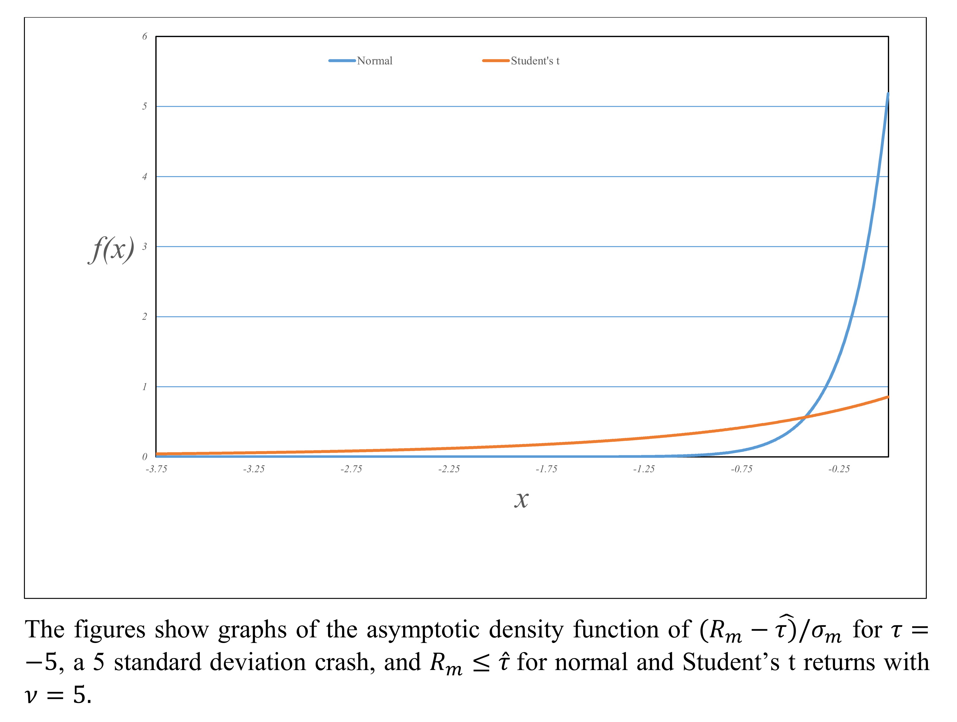
Using the results at Equation (78), it follows that the expected value of market return in a crash is negative and increases pro rata to the standardized crash size. Unlike the results based on an underlying normal distribution, the conditional variance is proportional to the square of the standardized crash size; for given $\nu$, the variance increases without limit. A sketch of the conditional distribution of index returns under normal and Student’s t distributions with five degrees of freedom and corresponding to a five-standard-deviation crash is shown in Figure 12. As the sketch shows, the Student’s t tail is longer and fatter than that of the normal.

The corresponding results for the conditional mean expected return vector is

$$E\left(\mathit{R}|R_m\le \tilde{\tau }\right)={\mathit{\mu }}_{\mathit{R}}-{\sigma }_m\mathit{\beta }{\xi }_{\nu }\left(\tau \right).$$

(93)

As above, the conditional expected return for asset i will increase or decrease without limit depending on the sign of ${\beta }_i$ but is unchanged if it equals zero. Using Equation (80), the conditional covariance matrix is

$$cov\left(\mathit{R}|R_m\le \tilde{\tau }\right)=\frac{\nu }{\left(\nu -1\right)}\left\{1+\frac{{\eta }_{\nu }\left(\tau \right)}{\nu }\right\}{\sum }_{\mathit{R}C}+{\sigma }_m^2\mathit{\beta }{\mathit{\beta }}^T\left\{{\eta }_{\nu }\left(\tau \right)-{\xi }_{\nu }{\left(\tau \right)}^2\right\},$$

(94)

which, in keeping with Equation (83), may also increase without limit. Noting that ${\eta }_{\nu }\left(\tau \right)=E\left\{{\left(R_m-{\mu }_m\right)}^2/{\sigma }_m^2|R_m\le \tilde{\tau }\right\}$, the similarities between Equation (94) and (88) are clear.

5. Extended Skew-Normal versus Skew-Student

The literature concerning the skew-normal and skew-Student distributions is more abundant that that for the corresponding extended versions. It has been conjectured by some researchers in the area, albeit informally, that the skew-Student could be used as an alternative to the extended skew-normal distribution. To some extent, such a suggestion is motivated naturally by the similarities in the shapes of some of the respective density functions. Somewhat more formally, use of the skew-Student could be regarded as being closer in spirit to the original skew-normal literature. For univariate distributions, and from the perspective of empirical work, this is an issue that is more concerned with parameter estimation and tests of fit. That is, for a given data set, does the extended skew-normal or the skew-Student offer better fit? For multivariate distributions, the issue is the same in principle, although the details are more complex. It is of course also the case that the extended skew-normal might be preferred to the skew-Student. For example, for the former, all moments exist, which may be a consideration for some applications. Conditional distributions are in general of the extended type. For multivariate applications in which conditioning is a requirement, methodological issues could imply that extended versions of the distribution are more appropriate. That is, an MESN or even MEST distribution may be preferable to the MST.

To construct an approximation, at least two types of method suggest themselves. Given a specified extended skew-normal distribution, one method would be to minimize a suitable measure of the distance between the two density functions. Several measures of distance could be considered. Denoting the two density functions by $f_{ESN}\left(x\right)$ and $f_{ST}\left(x\right)$ and assuming that the parameters of the former (latter) are given, the parameters of the latter (former) could be chosen by minimizing

$${\int }_{-\infty }^{\infty }{\left\{f_{ESN}\left(x\right)-f_{ST}\left(x\right)\right\}}^{2}dx.$$

Numerous variations on this theme could be constructed, for example, using a different norm or minimizing the divergence between the ESN and ST density functions using the Kullback–Leibler divergence measure [38] or the Hellinger distance ([39]). A second approach could be to seek to match the first four moments of the two distributions. It is clear that a comprehensive study of this conjecture, particularly bearing in mind multivariate distributions, would be a substantial undertaking. In this section of the paper, an initial investigation into the approximation of the univariate extended skew-normal distribution by the skew-Student, which may inform more comprehensive studies to be carrried out in the future, is described. The section is in two parts. In the first section, a theoretical investigation based on population moments is reported. In the second part, a study in which simulated data from a number of specified extended skew-normal distributions is used to estimate the parameters of both models is reported.

There are three technical points to note. First, the choice of an approximating skew-Student distribution is informed by the limiting forms of the extended skew-normal. From Lemma 1, as $\tau \to -\infty$, the limiting form of the ESN distribution is $N_n\left(\mathit{\mu },\sum \right)$, which is the limiting form of a skew-Student distribution with $\mathit{\lambda }=\mathit{0}$, that is, Student’s t, as $\nu \to \infty$. As also reported in Section 2, a similar result holds as $\tau \to \infty$. The implication is that using ST distributions to approximate the ESN is appropriate for values of $\left|\tau \right|$ that are not too large. Second, motivated again by similarities in the shape of the density function, an ESN distribution may be approximated by the SN itself. Third, there are combinations of the parameters $\lambda$ and $\tau$ for which approximation by moment matching are infeasible. To illustrate this, consider an approximation of a univariate ESN with parameters $\mu$, ${\sigma }^2$, $\lambda$ and $\tau$ by an SN with parameters ${\mu }_0$, ${\sigma }_0^2$ and ${\lambda }_0$. Equating skewness shows that a real value of the ratio ${\sigma }_0^2/{\lambda }_0^2$ requires that

$${\left\{{\xi }_3\left(0\right)\right\}}^{2/3}\left[{\sigma }^2/{\lambda }^2+\left\{1+{\xi }_2\left(\tau \right)\right\}\right]>{\left\{{\xi }_3\left(\tau \right)\right\}}^{2/3}\left\{1+{\xi }_2\left(0\right)\right\},$$

(95)

and that simple computations show that the inequality does not always hold.

5.1. Moment Matching Study

The study in this paper considers the approximation of an ESN distribution by an ST. As above, for the ESN, $\mu =0$ and ${\sigma }^2=1$. The extension parameter $\tau$ takes 11 values in the range $\left[-20,20\right]$. As skewness is asymmetric in the shape parameter; $\lambda$ takes 9 values in the range $[-10,0]$. For practical reasons, the derived value of $\nu$ is restricted to be an integer. For a given pair $\left(\lambda ,\tau \right)$, the approximating values of $\nu$ and ${\lambda }_0$ are derived by minimizing the absolute difference in standardized skewness. This is done by grid search. The other parameters are computed by equating the expected value and variance of the two distributions. For $\left(\lambda ,\tau \right)$, pairs for which a moment matching approximation exists, the divergence between the ESN and ST density functions is computed using the Kullback–Leibler divergence measure [38]. The values of this divergence measure are ranked from best to worst, with the parameters corresponding to the best ten and worst ten shown in

Table 11. Divergence between ESN ST density functions.

Panel 1: Kullback–Leibler divergence: Best 10
	$\lambda$	$\tau$	$\mu$[ST]	${\sigma }^2$[ST]	$\lambda$[ST]	$\nu$
	−0.5	−10.0	−0.0490	1.0024	0.0000	∞
	−0.5	0.0	0.0000	0.9999	−0.5000	∞
	−1.0	0.0	0.0000	0.9998	−1.0000	∞
	−1.5	0.0	0.0000	0.9998	−1.5000	∞
	−1.0	10.0	−10.0000	2.0000	0.0000	∞
	−0.5	10.0	−5.0000	1.2500	0.0000	∞
	−2.0	10.0	−20.0000	5.0000	0.0000	∞
	−3.0	10.0	−30.0000	10.0000	0.0000	∞
	−5.0	10.0	−50.0000	26.0000	0.0000	∞
	−1.5	10.0	−15.0000	3.2500	0.0000	∞
Panel 2: Worst 10
	−2.0	0.5	−0.9652	2.2017	−1.3000	50
	−2.5	0.5	−0.9208	2.5358	−2.0000	190
	−3.0	0.5	−1.0313	3.0917	−2.5000	∞
	−2.5	1.0	−2.0121	4.0001	−1.5000	90
	−2.5	−0.5	0.3925	0.4047	−2.5000	∞
	−3.0	1.0	−2.2658	5.1990	−2.0000	∞
	−5.0	−5.0	0.6725	0.3260	−2.0000	130
	−5.0	1.0	−4.8342	15.0568	−2.0000	150
	−5.0	0.5	−2.6469	9.7981	−3.0000	340
	−3.0	−0.5	0.4740	0.1265	−3.0000	500

The values of the Kullback–Leibler divergence measure are ranked from best to worst, with the parameters corresponding to the best ten and worst ten shown in the two panels. The first two columns of each panel show the values of λ and τ. The next three columns show the computed value of μ, σ², and λ for the approximating ST distribution, rounded to four decimal places. Computed values of ν equal to 1000 or greater were replaced by ∓, that is, the approximating distribution is effectively skew-normal.

. The first two columns of each panel show the values of $\lambda$ and $\tau$. The next three columns show the computed values of $\mu$, ${\sigma }^2$, and $\lambda$ for the approximating ST distribution, with values rounded to four decimal places. Computed values of $\nu$ that were equal to 1000 or greater were replaced by ∞, that is, the approximating distribution is effectively skew-normal.

Table 12. ESN and ST Moments.

Panel 1: Kullback–Leibler divergence: Best 10
	Mean	Variance	Skewness	Kurtosis	Mean (ST)	Variance (ST)	Skewness (ST)	Kurtosis (ST)
	−0.0490	1.0024	−0.0002	3.0142	−0.0490	1.0024	−0.0002	3.0142
	−0.3989	1.0908	−0.0273	3.5770	−0.3989	1.0908	−0.0275	3.5773
	−0.7979	1.3634	−0.2180	5.6912	−0.7979	1.3634	−0.2186	5.6917
	−1.1968	1.8176	−0.7358	10.4921	−1.1968	1.8176	−0.7371	10.4930
	−10.0000	2.0000	0.0000	12.0000	−10.0000	2.0000	0.0000	12.0000
	−5.0000	1.2500	0.0000	4.6875	−5.0000	1.2500	0.0000	4.6875
	−20.0000	5.0000	0.0000	75.0000	−20.0000	5.0000	0.0000	75.0000
	−30.0000	10.0000	0.0000	300.0000	−30.0000	10.0000	0.0000	300.0000
	−50.0000	26.0000	0.0000	2028.0000	−50.0000	26.0000	0.0000	2028.0000
	−15.0000	3.2500	0.0000	31.6875	−15.0000	3.2500	0.0000	31.6875
Panel 2: Worst 10
	−2.0183	2.9447	−2.1679	27.4245	−2.0183	2.9447	−2.1678	28.132
	−2.5229	4.0386	−4.2342	52.3748	−2.5229	4.0386	−4.2200	54.5273
	−3.0275	5.3756	−7.3167	93.8321	−3.0275	5.3756	−7.3482	99.0404
	−3.2190	4.9355	−4.6206	73.1000	−3.2190	4.9355	−4.5951	79.0081
	−1.6027	2.6780	−2.5407	25.539	−1.6027	2.6780	−2.5411	24.5375
	−3.8628	6.6672	−7.9844	133.3981	−3.8628	6.6672	−8.0281	147.2278
	−0.9325	1.8174	−1.3532	13.0888	−0.9325	1.8174	−1.3493	11.1028
	−6.4380	16.7422	−36.9648	841.2418	−6.4380	16.7422	−36.8354	940.0303
	−5.0458	13.1544	−33.8738	574.2185	−5.0458	13.1544	−33.8859	612.2122
	−1.9232	3.4163	−4.3903	43.3578	−1.9232	3.4163	−4.3974	41.1866

This table shows values of the moments corresponding to the parameters reported in Table 11.

shows the corresponding values of the moments. As the Best 10 panel shows, the differences in the first four moments are negligible. For the Worst 10 panel, differences in mean, variance, and skewness are also negligible because of the method of construction. Unlike the results in the upper panel, there are differences in kurtosis.

Table 13. ESN vs. ST critical values.

Panel 1: Kullback–Leibler divergence: Best 10
	0.5%ESN	ST	2.5%ESN	ST	97.5%ESN	ST	99.5%ESN	ST
	−2.65	−2.65	−2.05	−2.05	1.90	1.90	2.50	2.50
	−3.15	−3.15	−2.50	−2.50	1.60	1.60	2.25	2.25
	−4.00	−4.00	−3.20	−3.20	1.40	1.40	2.05	2.05
	−5.10	−5.10	−4.05	−4.05	1.25	1.25	1.90	1.90
	−13.65	−13.65	−12.80	−12.80	−7.25	−7.25	−6.40	−6.40
	−7.90	−7.90	−7.20	−7.20	−2.85	−2.85	−2.15	−2.15
	−25.80	−25.80	−24.40	−24.40	−15.65	−15.65	−14.25	−14.25
	−38.15	−38.15	−36.20	−36.20	−23.85	−23.85	−21.90	−21.90
Panel 2: Worst 10
	−63.15	−63.15	−60.00	−60.00	−40.05	−40.05	−36.90	−36.90
	−19.65	−19.65	−18.55	−18.55	−11.50	−11.50	−10.40	−10.40
	−7.05	−6.80	−5.75	−5.55	0.90	1.20	1.65	2.25
	−8.55	−8.20	−6.95	−6.70	0.80	1.20	1.60	2.25
	−10.05	−9.65	−8.20	−7.90	0.70	1.20	1.50	2.40
	−9.60	−9.20	−8.00	−7.70	0.55	1.05	1.35	2.35
	−6.75	−6.90	−5.30	−5.40	1.15	0.85	1.85	1.35
	−11.35	−10.80	−9.45	−9.10	0.40	1.05	1.25	2.55
	−5.30	−5.30	−3.95	−4.05	1.40	1.15	2.10	1.60
	−18.45	−17.20	−15.40	−14.55	0.00	1.50	1.00	4.00
	−16.30	−14.90	−13.30	−12.40	0.35	1.85	1.25	3.90
	−7.90	−8.05	−6.20	−6.35	1.05	0.55	1.80	0.90

The table shows critical values at p-values of 0.5%, 2.5%, 95.5%, and 99.5%, respectively, in ESN/ST pairs. Values are shown corrected to two decimal places and were computed numerically using Simpson‘s rule.

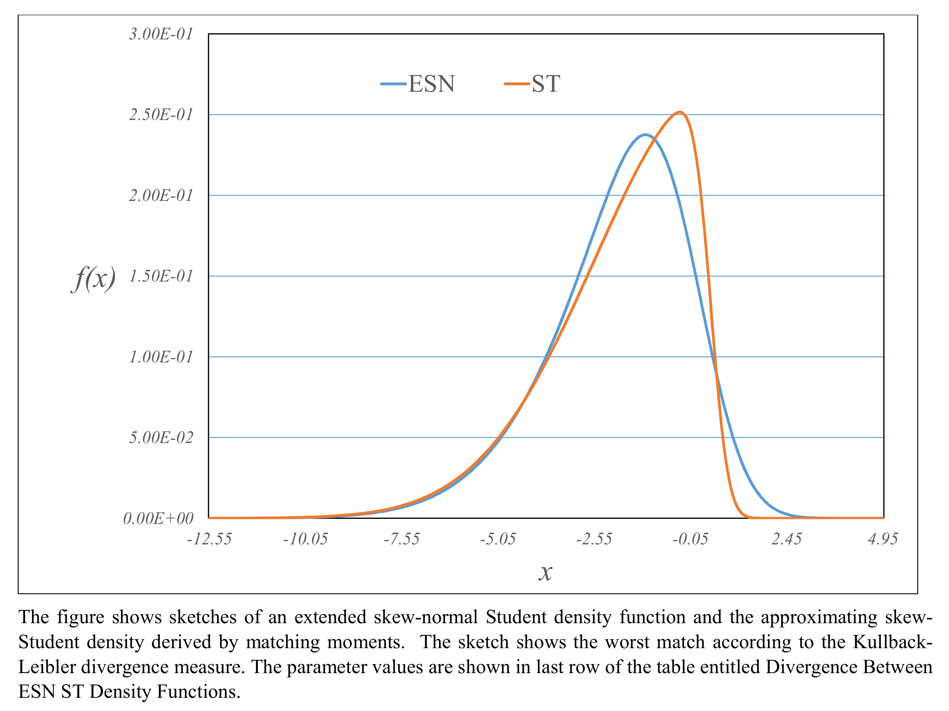
shows the corresponding critical values, displayed in eight columns. These show critical values at p-values of 0.5%, 2.5%, 95.5%, and 99.5% in ESN/ST pairs. Values are shown corrected to two decimal places and were computed numerically. As the table shows, for the Best 10 approximations, the differences are negligible. For the Worst 10, the differences are more pronounced. To illustrate the effect of the moment matching procedure, Figure 13 shows ESN and ST density functions for which the ST approximation is the worst according to the Kullback–Leibler divergence measure.

The results in Table 11, Table 12 and Table 13 provide support to the implications of Equation (95), namely that the method of approximations works well for values of $\left|\tau \right|$ that are not too large. An interesting result is that for numerous parameter combinations, the extended skew-normal distribution may be well approximated by a skew-normal. The usefulness of the results in the Worst 10 panels will depend on the application. In some applications, accurate critical values are not necessary, but in others, they are. There are other methods of measuring the divergence between two density functions. Two well-known ones are Hellinger distance ([39]) and Jensen–Shannon divergence ([40]), both of which constitute topics for future investigation.

5.2. Simulation Study

The simulation study uses the same sets of values of $\mu$, ${\sigma }^2$, $\lambda$, and $\tau$. For each combination of the parameters, 100 samples of size 100 from an extended skew-normal distribution were drawn. The parameters were estimated by maximum likelihood for the ESN and ST distributions. In addition, motivated by the results in Table 11, the parameters of the skew-normal distribution were also estimated. Summaries of the results are shwon in

Table 14. Summary of estimated log-likelihood function.

	Sample	MLE (ESN)	MLE (ST)	MLE (SN)
−2.5	−162.1227	−143.8078	−143.7856	−144.2421
−1	−166.7300	−147.7064	−148.1087	−148.2171
−0.5	−173.5951	−154.3467	−154.7982	−155.0793
0	−181.6436	−162.3594	−162.5675	−163.1677
0.5	−190.3665	−171.9357	−172.3604	−172.6343
1	−199.0348	−180.9025	−180.4694	−181.2470
2.5	−199.5184	−181.6458	−181.8682	−182.0044

The table shows the value of the log-likelihood function for each parameter combination computed at its estimated maximum, averaged over the 100 samples and over values of τ. Column 1 shows values of logL based on parameter values inferred from sample moments. As columns 2 through 4, the value of logL varies little with the choice of underlying distribution.

,

Table 15. Root mean square errors in the moments.

Panel 1: $\mathit{\lambda }=-2.5$
	MLE (ESN)	MLE (ST)	MLE (SN)
$\tau =$−5.0	0.0173	0.2864	0.0733
−2.5	0.3679	0.2720	0.3626
−1.0	0.9311	0.6039	0.9170
0.0	0.6527	5.3254	0.6702
1.0	3.0086	8.1842	5.8937
2.5	5.8728	8.7935	6.9017
5.0	3.8259	6.4790	5.7127
Panel 2: $-\mathit{1}$
−5.0	0.0878	0.2736	0.1137
−2.5	0.0851	0.3863	0.1398
−1.0	0.0630	0.2508	0.0838
0.0	0.0528	0.3052	0.0915
1.0	0.2190	0.5452	0.3016
2.5	0.4006	1.0383	0.4772
5.0	0.3251	0.6928	0.3406
Panel 3: 0
−5.0	0.0751	0.3443	0.1084
−2.5	0.1038	0.3784	0.1294
−1.0	0.0797	0.4221	0.1050
0.0	0.0979	0.4147	0.114 0
1.0	0.0898	0.4213	0.1257
2.5	0.1162	0.5211	0.1340
5.0	0.0752	0.2855	0.1242
Panel 4: 1
−5.0	0.0709	0.3994	0.0769
−2.5	0.0651	0.3919	0.1001
−1.0	0.0664	0.4552	0.1297
0.0	0.1606	0.5150	0.1971
1.0	0.3868	0.8329	0.3099
2.5	0.3001	1.0357	0.3504
5.0	0.2648	1.4494	0.3207
Panel 5: 2.5
−5.0	0.1321	0.5672	0.1594
−2.5	0.4829	0.9696	0.8214
−1.0	0.7027	2.3434	2.1031
0.0	0.7355	3.7407	2.8966
1.0	3.3669	9.8534	2.1806
2.5	4.9614	14.3890	5.0747
5.0	1.9213	15.8112	2.5600

Root mean square error is computed as the square root of the average squared difference between the population moments and the average of the estimated moments based on MLE parameter estimates for each distribution. The population moments included in the calculations are mean, variance, skewness, and kurtosis.

and

Table 16. Root mean square errors in the critical values.

Panel 1: $\mathit{\lambda }=-2.5$
	MLE (ESN)	MLE (ST)	MLE (SN)
$\tau =$−5.0	0.0812	0.059	0.0932
−2.5	0.2294	0.2106	0.2017
−1.0	0.2158	0.2109	0.2074
0.0	0.0407	0.342	0.0361
1.0	0.1459	0.5914	0.2343
2.5	0.2971	0.465	0.2715
5.0	0.0668	0.1735	0.3859
Panel 2: $-\mathit{1}.\mathit{0}$
−5.0	0.0336	0.0765	0.1295
−2.5	0.0492	0.0676	0.1692
−1.0	0.0610	0.0457	0.1172
0.0	0.0547	0.0892	0.0849
1.0	0.0715	0.1072	0.1381
2.5	0.0436	0.1564	0.1600
5.0	0.0331	0.0808	0.1662
Panel 3: 0
−5.0	0.0131	0.0830	0.1360
−2.5	0.0365	0.0956	0.1347
−1.0	0.0185	0.1062	0.1427
0.0	0.0260	0.0786	0.1465
1.0	0.0190	0.1070	0.1452
2.5	0.0445	0.1282	0.1184
5.0	0.0486	0.0824	0.1750
Panel 4: 1
−5.0	0.0335	0.0782	0.1309
−2.5	0.0243	0.0481	0.1753
−1.0	0.0516	0.0807	0.2266
0.0	0.0649	0.1004	0.2440
1.0	0.0506	0.0925	0.2430
2.5	0.0468	0.1542	0.2263
5.0	0.0203	0.1498	0.1910
Panel 5: 2.5
−5.0	0.0544	0.0516	0.2556
−2.5	0.2504	0.2543	0.5273
−1.0	0.2045	0.2328	0.7658
0.0	0.0512	0.2558	0.8942
1.0	0.1020	0.5654	0.9505
2.5	0.2790	0.5385	0.6304
5.0	0.1155	0.3089	0.3715

Root mean square error is computed as the square root of the average squared difference between the population critical values and the average of the estimated values based on MLE parameter estimates for each distribution. The critical values are computed at nominal percent probabilities equal to 0.05, 0.5, 2.5, 5.0, 95.0, 97.5, 99.5, and 99.95.

. Table 14 shows the value of the log-likelihood function for each parameter combination computed at its estimated maximum, averaged over the 100 samples and over values of $\tau$. The table has four columns, with the first showing values of $logL$ based on parameter values inferred from sample moments. As columns 2 through 4 of the table show, the value of $logL$ varies little with the choice of underlying distribution. For this relatively small sample size, if the value of $LogL$ were the sole criterion for model selection, it would be difficult to discriminate between the three distributions.

For each parameter combination shown in Table 15 and Table 16, the entries are averages of the 100 samples. Table 15 shows the root mean-square error in the moments for the three distributions and for 35 selected combinations of $\left(\lambda ,\tau \right)$. As the table shows, the lowest root mean-square error occurs under the ESN for 30 of the $\left(\lambda ,\tau \right)$ combinations. Root mean square error is computed as the square root of the average squared difference between the population moments and the average of the estimated moments based on parameters based on MLE for each distrbution. The population moments included in the calculations are mean, variance, skewness, and kurtosis. Table 16 shows the corresponding errors in the critical values. Root mean square error is computed as the square root of the average squared difference between the population critical values and the average of the estimated values based on MLE parameter estimates for each distribution. The critical values are computed at nominal percent probabilities equal to 0.05, 0.5, 2.5, 5.0, 95.0, 97.5, 99.5, and 99.95. The lowest root mean square error occurs under the ESN for 28 of the parameter combinations. In both Table 15 and Table 16, the root mean square error is generally the largest under the ST distribution.

6. Concluding Remarks

In this paper, results that demonstrate the properties of both the multivariate extended skew-normal and extended skew-Student distributions as the value of the extension parameter $\tau$ changes are presented. In general, for given value of location, scale, and shape or skewness, nonzero values of $\tau$ lead to greater variability in both the moments and critical values. In turn, this offers greater flexibility in empirical applications of these distributions. From a theoretical perspective, increasing values of $\left|\tau \right|$ leads to more fundamental changes in both distributions. As $\tau$ increases without limit, the asymptotic distributions are multivariate normal and multivariate Student, respectively. The respective vectors of expected values of both distributions are dependent on $\tau$ and are unbounded. The covariance matrices, however, remain finite. Skewness disappears for both distributions. By contrast, as $\tau \to -\infty$, more substantial changes take place in the distributions. Most notable is that for the MESN distribution dependence on $\tau$ vanishes, but for the MEST in general, it does not. In the case of the MESN, the limiting distribution is multivariate normal. For the MEST distribution with finite degrees of freedom, asymmetry remains. For fixed $\tau$, the extent of asymmetry decreases as the degrees of freedom increase. For fixed degrees of freedom, as $\tau \to -\infty$, the vector of expected values and the covariance matrix are both unbounded.

To illustrate the potential of the MESN and MEST distributions, two applications are described. First, the effect of a stock market crash is studied assuming underlying multivariate normal and multivariate Student distributions. A crash, in which the return on a market index is less than a given negative threshold, results in multivariate extended skew-normal and multivariate extended skew-Student distributions. Under an underlying multivariate normal distribution, as the crash size increases without limit, the return on a stock market index becomes nonstochastic. In short, the market plummets: actual return equals expected return. Under an underlying multivariate Student distribution, expected return is broadly the same, but variability increases without limit. The market decline is noisy. There are analogous results for the returns on individual stocks. In particular, with underlying normality, the conditional covariance matrix remains finite, whereas under an underlying Student distribution, it does not. A detailed investigation of the implications and suitability of these models is beyond the scope of this particular paper, but it is reasonable to posit that the results offer support to the view that an underlying Student distribution is a more realistic model than the normal. Given that stock market collapses have in the past been of relatively short duration, the results also imply that for financial applications the models change. The methods described may be applied in principle to stock market booms. It may also be noted that if an inefficiency variable were to be constructed, SFA analysis could be treated in the same way.

Second, the conjecture that the skew-Student could be used instead of the extended skew-normal is an interesting one. Given the similarity in the shapes of the density functions for many combinations of parameters, this conjecture suggests that there is the possibility of flexible model choice. A general investigation of this conjecture would be a substantial task. The exercise reported in this paper is intended to offer evidence to motivate further research. The short study reported in this paper, part theoretical and part based on simulation, suggests that a given ESN distribution should be treated as such. However, the results also suggest that the ESN could be well-approximated by the skew-normal in some circumstances, but in general not by the skew-Student.