1. Introduction
The analysis of time series has enjoyed sustained interest, in particular the case when the data generating process emanates from an underlying counting model, resulting in the considered innovation process to follow some stochastic discrete distribution. Practical examples of such scenarios include the number of daily transactions on a stock exchange, number of days patients spend in a health care facility, or the daily counts of positive COVID-19 cases in a specific geographical area.
Under this discrete innovation assumption, the often considered assumption of normality leaves the practitioner in an unideal position due to this continuous assumption for a process which is inherently discrete in nature. In particular, Ref. [
1] provides a seminal guideline on the use and implementation of a discrete-based time series analysis with discrete innovations, and various authors (such as [
2,
3,
4,
5] and others) have considered the first-order integer-valued (stationary) autoregressive process (INAR(1)) as a more viable contender compared to the usual (continuous) first-order autoregressive process (AR(1)), where the error term
is oftentimes characterised by a Poisson random variable. Suppose that
represents the (non-negative) discrete time series count at time
t (
), then the INAR(1) process is defined by
where
and ∘ denote the binomial thinning operator, defined by
where
is a Bernoulli random variable such that
. For the innovations
in (
1), the mean is indicated by
and finite variance by
; and for the INAR(1) model itself in (
1), the mean is given by
and the variance by
(see also [
1,
6,
7]). The choice of the Poisson model for
was introduced by [
8], but has been shown to be inefficient for accurate inference due to the equidispersion property, where
of the Poisson distribution.
To address this, Refs. [
6,
9,
10,
11] introduced alternative considerations for the choice of
, some of which emanates from the Lindley distribution or its generalisations incorporated into a discrete model for the INAR(1) innovation process. The Lindley distribution in itself has shown significant versatility as a continuous lifetime model, and a variety of generalisations of this model has been studied and reported on in literature (see [
12,
13,
14]). In addition to this, the incorporation of the Lindley distribution and its generalisations within a Poisson framework to obtain generalised discrete models has also experienced a sustained interest, mainly due to the attractive feature of being able to model departures that data might exhibit from equidispersion. In this study, a meaningful noncentrality parameter is systematically induced into the Lindley distribution from where a discrete counting model is also derived. This counting model is then illustrated as a candidate for
within a discrete time series environment. In this way, this work enriches the existing literature with a previously unconsidered noncentral candidate with a parameter that has leverage and meaning within understanding and modelling dispersion in discrete models, apart from a standalone contribution to the ever-growing literature on statistical distribution theory.
Therefore the contribution of this paper is threefold:
A noncentral Lindley distribution is systematically constructed and some statistical characteristics are derived;
A discrete counting model based on this noncentral Lindley distribution is derived via compounding with the Poisson distribution, together with essential statistical characteristics;
This discrete counting model is implemented and illustrated as innovation structure (i.e., ) within an INAR(1) time series environment, and juxtaposed against often-considered contenders for the innovation structures.
The particular value of interpretable and systematically induced noncentrality in these contributions is highlighted. These contributions pave the way for flexible statistical modelling in practice not only for meaningful inference, but also continuing the understanding, expansion, and development of the statistical theoretic universe. These models, as competitors, exhibits meaningful and tractable choices for the practitioner to employ within not only usual positive real-data modelling, but also discrete modelling, and thirdly, within an INAR counting time series environment.
The paper is outlined as follows. In
Section 2, the systematic construction of the noncentral Lindley (ncL) distribution is discussed and characteristics of this model are derived, followed by the construction and characteristics of the Poisson-noncentral Lindley (PncL) model.
Section 3 describes and contains the modelling results of applying the newly developed models to real data, including a fitting and discussion around the implementation of the PncL within the INAR(1) (
1) model. The final thoughts are contained in
Section 4.
2. Building Blocks of New Model
The Lindley distribution (initially introduced by [
15]) has seen a resurgence of attention over the span of the last 15 years, which could be attributed to its elegant construction as a weighted two-mixture distribution. This mixture consists of an exponential distribution with parameter
as the first component (with density function denoted by
), and a gamma distribution with scale and shape parameters
(with density function denoted by
). The weight function for this two-mixture distribution is given by
. In this paper, we consider a generalised weight function with additional parameters
and
for additional flexibility; that is,
where
and
(see [
3,
16]). This leaves a random variable
Y with density function:
Our point of departure for the contribution of this paper is to consider a noncentral gamma distribution with noncentral parameter
instead of the usual gamma choice in (
2). This leads to our proposed noncentral Lindley construction (ncL) construction, defined below.
2.1. A Noncentral Lindley Construction
We construct an ncL distribution by considering a random variable
Y which follows the noncentral gamma distribution with scale, shape, and noncentral parameters
with density function (see [
17]):
where
denotes the gamma function. Various authors (see for example, [
17,
18,
19,
20]) have considered and employed the noncentral gamma distribution as an essential generalisation of the gamma distribution, and also as a direct generalisation which emanates from the popular noncentral chi-square distribution. In particular, the hierarchical representation of (
3) is theoretically attractive as a discrete mixture of the (usual) gamma distribution.
The consideration of this noncentral gamma distribution (
3) as an enriched mixture component in (
2), instead of the usual gamma distribution, is thus a systematic and organic parameter enrichment to result in a noncentral Lindley alternative. In this case, the density function of the resulting ncL distribution is given by:
where
denotes the confluent hypergeometric function, and
denotes the Pochammer coefficient (see [
21]). In this case, we denote
. When
, (
4) reduces to the considered generalised Lindley model of [
3] with density function (
2). Furthermore, when
, (
4) reflects the usual Lindley density function (see [
15]).
The distribution function, moment generating function, and moments of
with density (
4) is presented in the following theorem. The proof is contained in
Appendix A.
Theorem 1. Suppose that the random variable Y is distributed as ncL with density function (4). Then, the distribution function, moment generating function, and moments of Y is given by: where , , denotes the incomplete lower gamma function (see [21]) and represents the hypergeometric function with one lower and one upper parameter (see [21]). Note that in (5) may be simplified further into a closed form as using [21], equation 8.352.6. These expressions exhibit the elegant incorporation of the noncentral parameter
, and using all three characteristics (
5), (
6), and (
7) by setting
, the corresponding characteristics of the usual generalised Lindley of [
22] (see also [
3]) may be obtained.
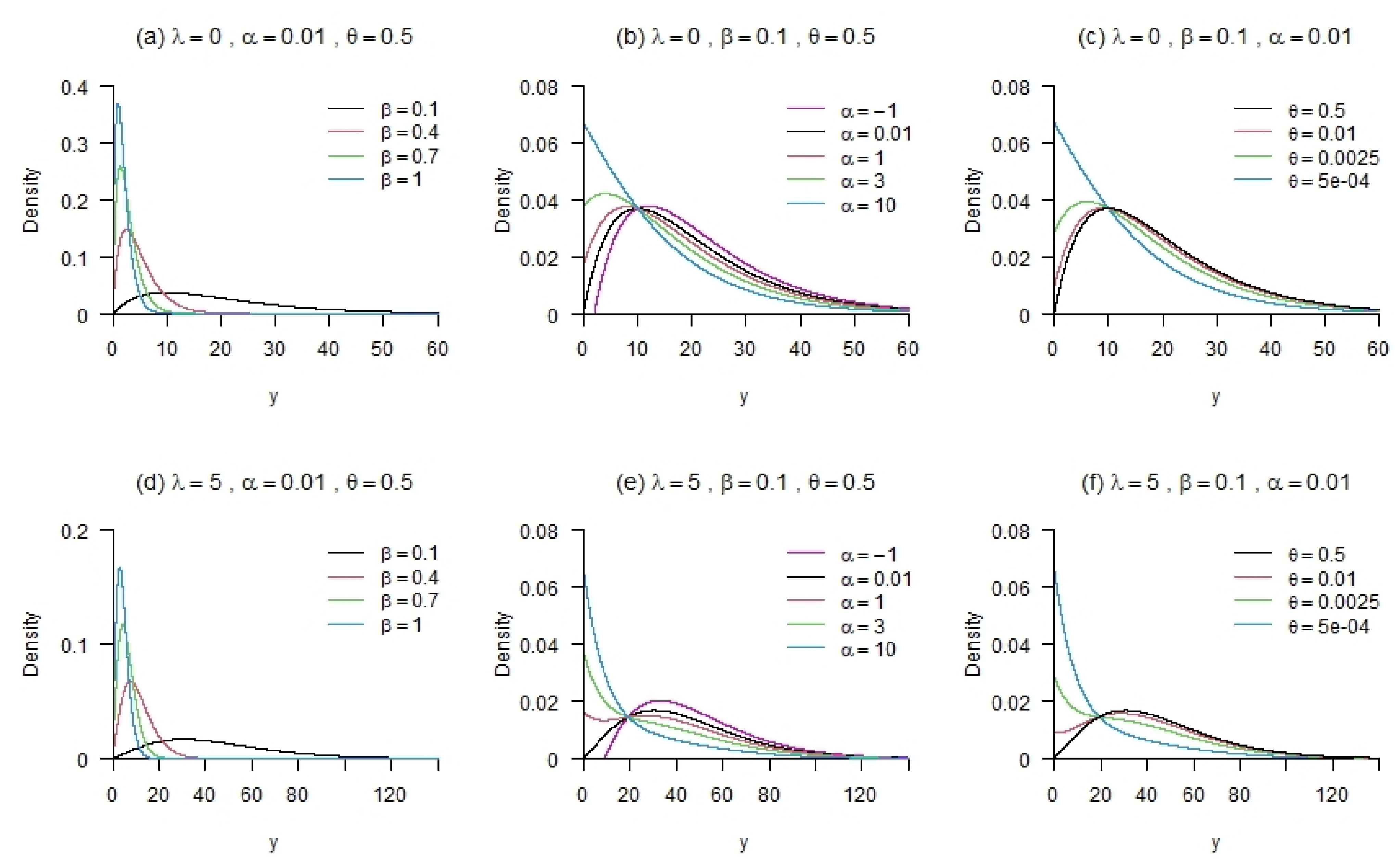
In
Figure 1, some particular shapes of the density function (
4) are illustrated for various combinations of parameters. The following effects are observed for changes in the different parameters:
2.2. A Counting Model: PncL Distribution
For discrete (count data) modelling, the Poisson distribution is a well-known and popular choice due to its tractability and ease of implementation. The author of [
23] illustrated the possibility of allowing the Poisson parameter (say
) to be distributed according to the Lindley distribution of [
15], and investigated characteristics related to this. When considering the dispersion index
, it is noted that the equidispersion property (when
) of the Poisson distribution is often restrictive—in this sense, the contribution of the ncL distribution as a viable candidate for the distribution of the Poisson parameter
is discussed in this section. This proves to be particularly valuable and directly insightful as the practitioner may allow for leverage on the mean (or rather, noncentrality) of the model via the use of
and thus inherently be able to model departures from equidispersion which the data may exhibit.
Suppose a variable
X follows a Poisson distribution with parameter
, and let
be distributed as ncL with a density function as in (
4). Then, using the compounding method with [
21], the mass function for
X is given by:
for
representing counts. In this case, we define
.
The probability generating function and factorial moments of the distribution in (
8) are presented in the following theorem. The proof is contained in
Appendix A.
Theorem 2. Suppose that the random variable X is distributed as a PncL variable with mass function (8). Then, the probability generating function and factorial moment of X are given by: where and . Note that by replacing s with in (9), the moment generating function of the distribution in (8) is obtained. Our systematically constructed discrete model includes the model of [
23] as a special case, particularly when
and
and also reflects a similar model as that of [
3]. It is, however, important to note that [
3] relied on the survival discretisation method instead of compounding to obtain a discrete candidate based on their considered underlying generalised Lindley model.
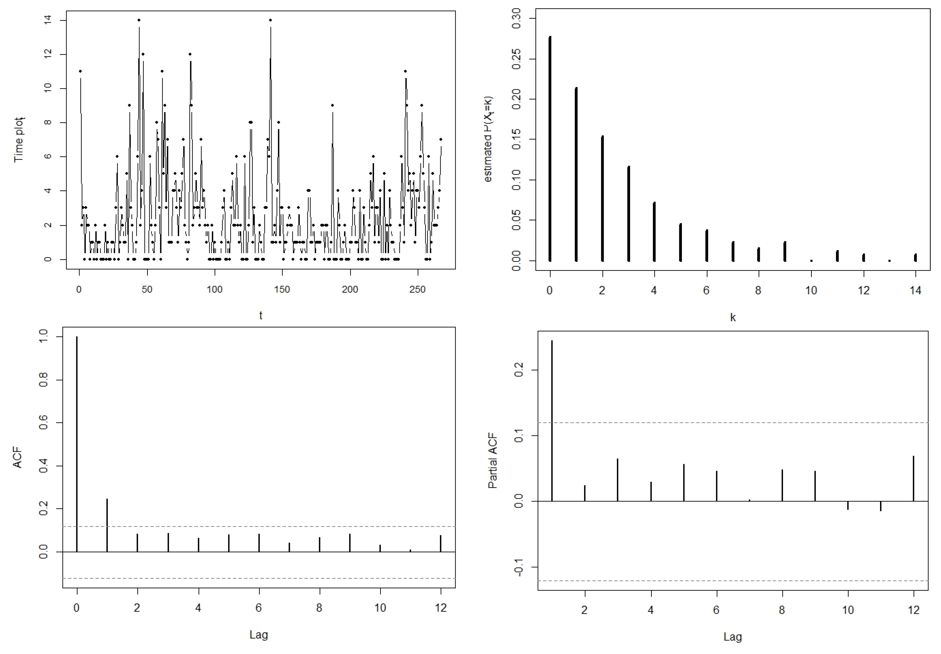
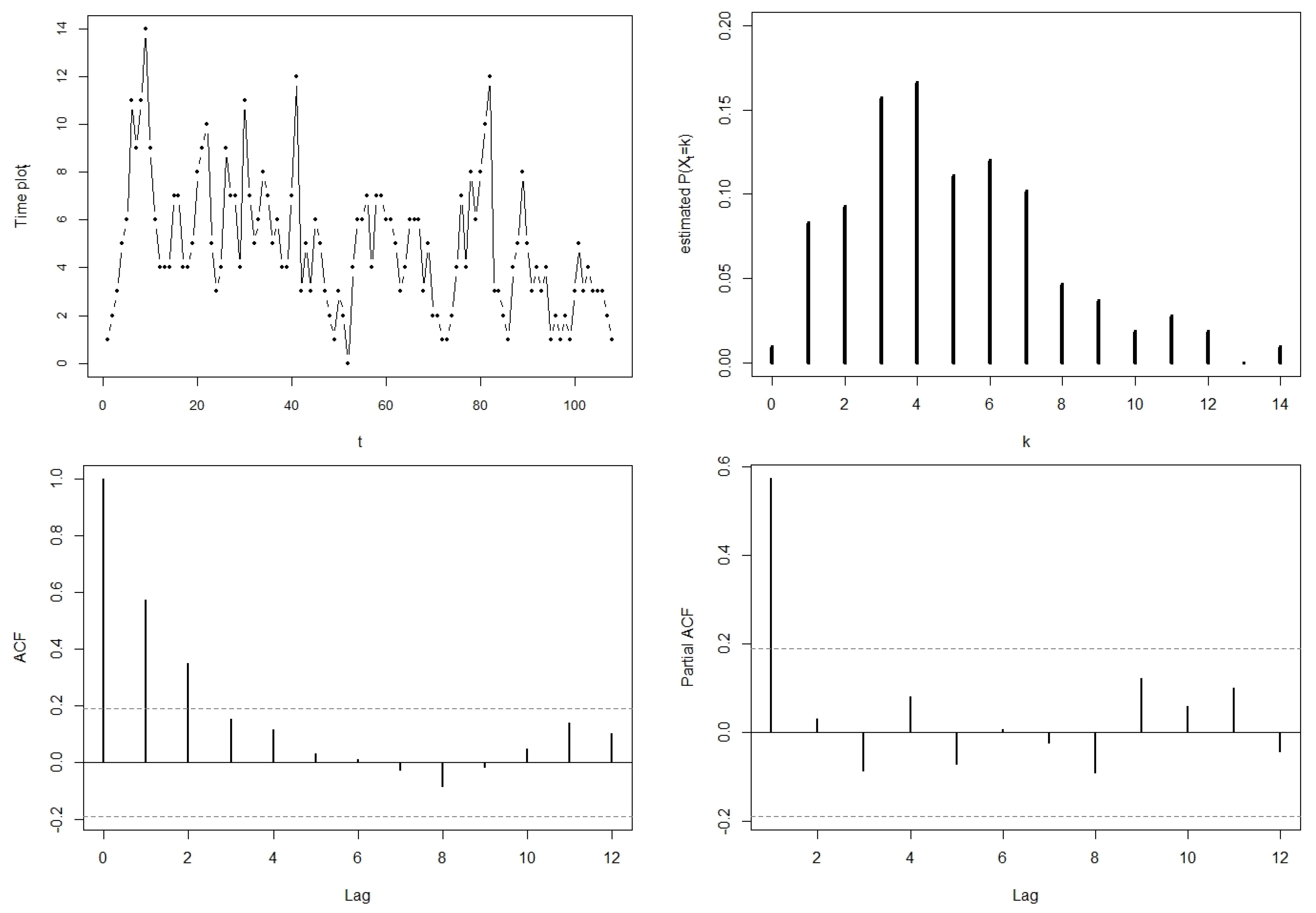
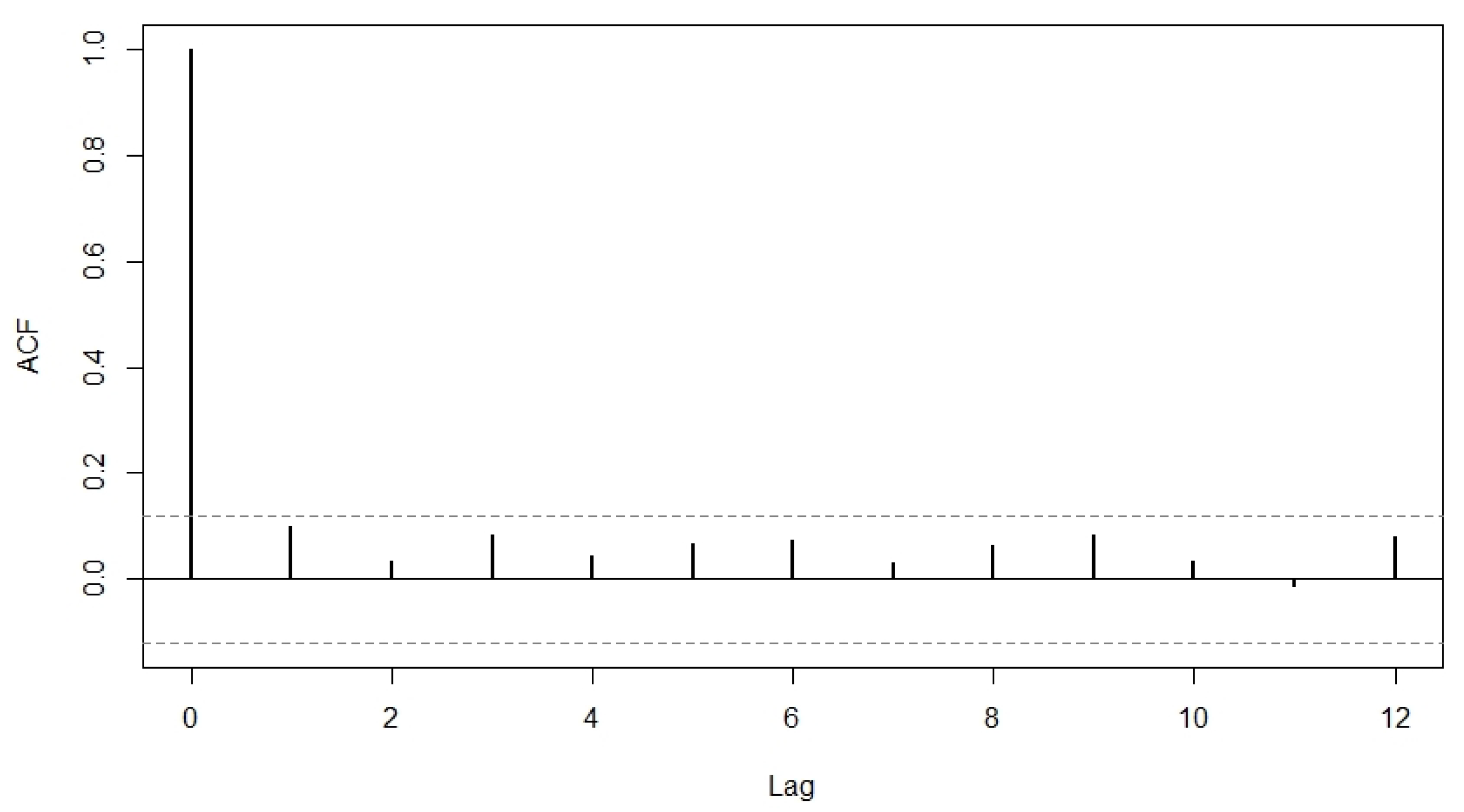
Table 1 illustrates the behaviour that can be captured by the PncL model (
8) by calculating the theoretical values of the mean, variance,
, skewness, and kurtosis for different values of
. It is valuable to note the correspondence between the mean and
in particular, as this provides a unique insight for the practitioner of the leverage related to the
via the incorporation of
. In this case, the skewness and kurtosis of the variable
X is given by
and
, respectively, and calculated using the moments (
A1)–(
A4) as given in
Appendix B.
In addition to
Table 1,
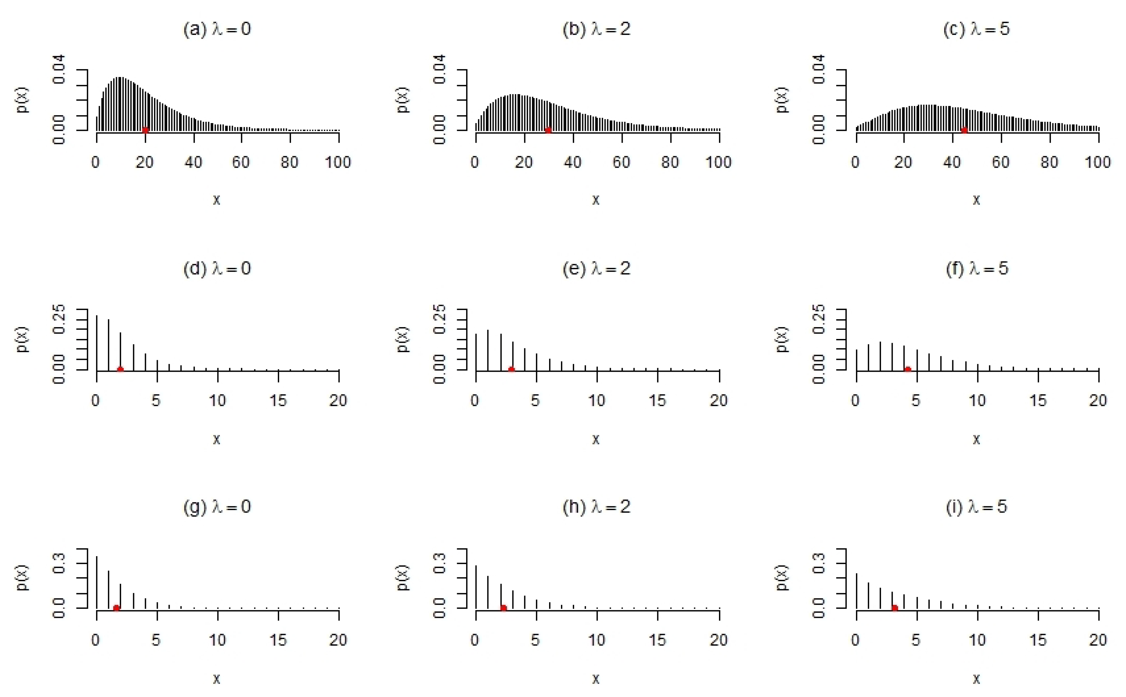
Figure 2 illustrates some particular shapes of the mass function (
8) for different values of
for the following combinations of
,
, and
:
,
and
, illustrated in
Figure 2a–c;
,
and
, illustrated in
Figure 2d–f;
,
and
, illustrated in
Figure 2g–i.
The following is observed from
Figure 2:
affects the location (evident from the shifts in the means illustrated in red) and spread of the distribution. As
increases, the distribution flattens out, shifts to the right and becomes less skewed. This is also evident from
Table 1;
affects the scale of the distribution. As
increases, the scale of the distribution increases (comparing the mass functions in
Figure 2a–c to
Figure 2d–f, respectively);
and
jointly affect the shape of the distribution (comparing the mass functions in
Figure 2d–f to
Figure 2g–i, respectively).
Figure 2.
Shapes of the mass function (
8) for arbitrary parameter choices, with means indicated in red. (
a–
i) some particular shapes of the mass function (
8) for different values of
for the following combinations of
,
, and
.
Figure 2.
Shapes of the mass function (
8) for arbitrary parameter choices, with means indicated in red. (
a–
i) some particular shapes of the mass function (
8) for different values of
for the following combinations of
,
, and
.
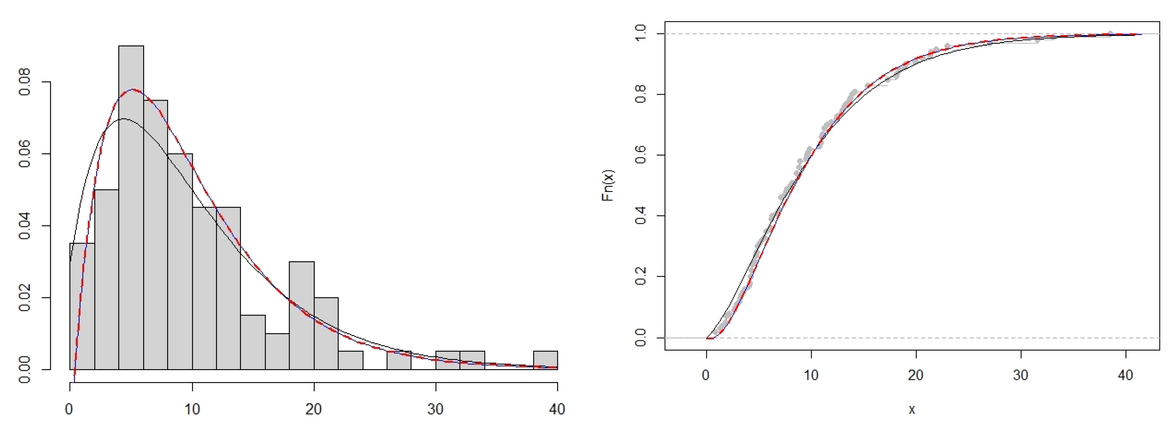
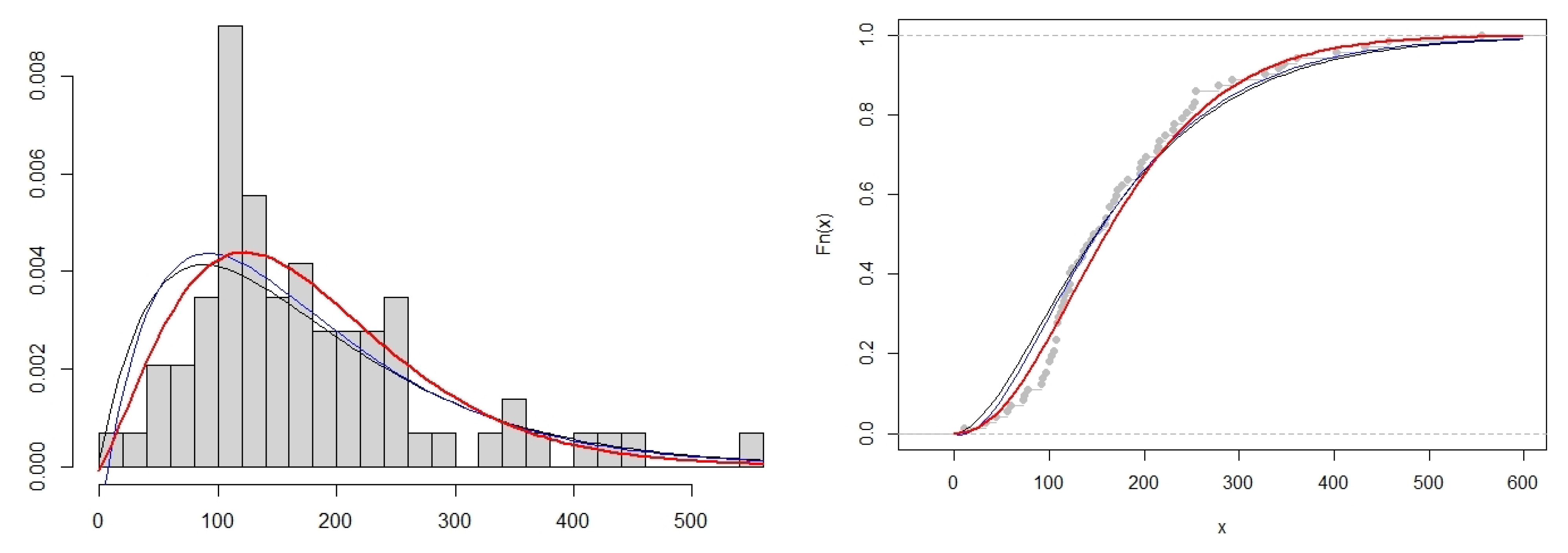
4. Conclusions
This study presents an enriched noncentral Lindley distribution (ncL) containing a (noncentral) parameter which has been systematically introduced via the noncentral gamma distribution. The characteristics of this newly developed model received attention, which includes the cumulative distribution function, moment generating function, and the moments of the distribution which are derived in closed form analytical expressions. This model retains mathematical elegance with closed forms for the characterisations, and is shown to contain existing models in the literature for specific choices of the parameters. In addition, a discrete counterpart was derived by using this ncL model via compounding with a Poisson variable. In this way, the interpretability of the noncentral parameter is inherited within a discrete environment as well, and paves the way for the practitioner to leverage information regarding the mean (or rather, noncentrality) of any suitable given data to provide insight on the dispersion index of the data in question. This model is incorporated within a time series context as innovation terms in an INAR(1) environment and juxtaposed against other popular models.
It is valuable to note that no one distribution will always outperform another, due to the data-driven nature of statistical model fitting. As such, the contributions in this paper does not exclusively outperform competing models in terms of the considered datasets—but results indicate that it is as good a model, if not occasionally slightly better, than the usual choices. The true value of this paper lies within this systematic construction of a previously unconsidered continuous (ncL) and discrete (PncL) distribution, and the inclusion of a noncentral parameter which is estimable and interpretable in a location context for data. Additionally, these models contain usual considered models as special cases, and thus acts as a unifying consideration for practitioners not only with continuous or discrete interests, but also with discrete time series interests. In future, further considerations and comparisons of other unconsidered discrete models (such as the refreshing recent contribution of [
28] as well as [
29]) within a discrete time series environment may be pursued, in conjunction with alternate thinning considerations (such as [
30]).


