A Bayesian Approach for Imputation of Censored Survival Data

Abstract

A common feature of much survival data is censoring due to incompletely observed lifetimes. Survival analysis methods and models have been designed to take account of this and provide appropriate relevant summaries, such as the Kaplan–Meier plot and the commonly quoted median survival time of the group under consideration. However, a single summary is not really a relevant quantity for communication to an individual patient, as it conveys no notion of variability and uncertainty, and the Kaplan–Meier plot can be difficult for the patient to understand and also is often mis-interpreted, even by some physicians. This paper considers an alternative approach of treating the censored data as a form of missing, incomplete data and proposes an imputation scheme to construct a completed dataset. This allows the use of standard descriptive statistics and graphical displays to convey both typical outcomes and the associated variability. We propose a Bayesian approach to impute any censored observations, making use of other information in the dataset, and provide a completed dataset. This can then be used for standard displays, summaries, and even, in theory, analysis and model fitting. We particularly focus on the data visualisation advantages of the completed data, allowing displays such as density plots, boxplots, etc, to complement the usual Kaplan–Meier display of the original dataset. We study the performance of this approach through a simulation study and consider its application to two clinical examples.

1. Introduction

The primary interest in survival analyses in clinical studies is studying the time to an event such as death or disease recurrence. In survival analysis subjects are followed for a fixed period of time. Unless this follow-up continued until everyone in the study had experienced the event, some patients will be event-free (i.e., censored) and their time to event will remain unknown. As a consequence of censoring, standard methods for plotting survival times (a continuous response variable) such as a histogram, density or boxplot are not suitable. Graphical displays of time-to-event data usually take the form of a plot of the survivor function, typically using the Kaplan–Meier estimator.

Despite its widespread use, a plot of the estimated survival function might not be the most informative way to present such a response. In a similar manner, the median survival time (the time that 50% of the sample survived to) is a popular summary reported to a patient whose importance has been questioned [1] and is not estimable in the case of extensive censoring.

When using plots of survivor functions to compare treatment groups, divergence between the plots at larger follow up times may be mistakenly interpreted as a dramatic benefit of a treatment unless a measure of uncertainty, such as a confidence interval or alpha blending [2], is included to indicate uncertainty due to small sample sizes. The smaller the number of people available to experience an event, the larger the drop when there is an occurrence of an event. Two estimated survivor functions may look very different, accompanied by a small log-rank p-value, but the actual distribution of time to events may overlap considerably. A simple example of this is when one of the distributions is a scale/location shift of the other; the Kaplan–Meier curves will be distinct, non-overlapping and significantly different, for sufficiently large samples; however, the actual distributions will overlap with the bulk of the support given to common event times, particularly if the scale/location shift is not too large. Providing graphical summaries of the underlying distribution of the time to the event is clearly an attractive addition to provide clarity and help to avoid mis-interpretations.

The aim of this paper is to consider censored data as a form of missing data and use approaches from the missing data literature to impute censored observations in order to use graphical techniques for complete data to summarise time to event data in more informative and translatable ways. The imputation of censored observations not only allows more interpretable graphics to be produced, but it also opens the possibility of the use of formal methods of analysis for continuous responses. Here the focus is on demonstration of the method and uses simple examples to show the feasibility and usefulness of a Bayesian imputation approach. Further detail will be reported in a subsequent manuscript.

The paper proceeds as follows: In Section 2 methods for imputing censored observations are reviewed and a new method using a Bayesian approach is presented. The results of a simulation study to assess the performance of this method are given in Section 3, Section 4 presents the application of the method to two different case studies, and concluding remarks are given in Section 5.

2. Imputing Censored Observations

The idea of imputing right censored survival data have, to some extent, already been considered in the literature. Wei and Tanner [3] proposed a method to impute failure times for censored observations drawn from the conditional normal distribution in the context of regression analysis with censored data. Moreover, in another paper [4], they used the Poor Man’s data augmentation algorithm and an asymptotic data augmentation algorithm for censored regression data. Furthermore, Pan and Connett [5] have extended these results to clustered censored data in semi-parametric linear regression models. Ageel [6] considers using an estimated value of $E\left[T_i\right|T_i>C_i]$ as a pseudo-value to replace the ith censored observation using both an empirical distribution and the Weibull distribution. Furthermore, Chiou [7] proposed a method where censored observation are imputed by Median $[T_i\mid T_i>C_i]$. Cantor [8] presented a method of imputation for right censored survival data based on a Gompertz model in which the possibility that an individual with a censored survival time is cured is explicitly accommodated. Lue et al. [9] addressed the issue of reducing the dimension of predictors in survival regression without requiring a pre-specified parametric model by replacing each right censored survival time with its conditional expectation using Buckley and James [10] pseudo-random variables $Y_i=T_i{\delta }_i+E[T_i\mid T_i>C_i](1-{\delta }_i)$. Jackson et al. [11] imputed failure times for censored participants from the entire sample of observed failure times that are greater than their corresponding censoring times in order to quantify the sensitivity of the conclusions from fitted Cox proportional hazards models.

Royston [12,13] presented a method to impute each censored survival time by assuming a lognormal distribution for the unobserved actual failure time. Taylor et al. [14] described non-parametric multiple imputation methods, including risk set imputation and Kaplan–Meier imputation, to handle missing event times for censored observations in the context of non-parametric survival estimation and testing. Faucett, Schenker and Taylor [15] and also Hsu in collaboration with Taylor and other colleagues [16] used auxiliary variables to recover information from censored observations by using Markov chain Monte Carlo methods to impute event times for censored cases. Hsu and Taylor [17] extended this work on estimation using auxiliary variables to adjust, via multiple imputation, for dependent censoring in the comparison of two survival distributions. Hsu, Taylor and Hu [18] further adapted their method to the situation where the event and censoring times follow accelerated failure time models.

The approach proposed in this paper uses a parametric Bayesian framework to impute right censored observations. The Bayesian approach would be appropriate as historical data from similar past studies can be very helpful in interpreting the results of the current study. In particular, we will use the idea of imputing the censored observations, based on the other information in the dataset and some form of model. However, in using imputation for censored data, there is an important difference from standard missing data imputation, with censored data we have some, albeit limited, information on the censored value. In right censoring the true failure times exceeds the recorded censored time and we use this information in our imputations.

2.1. Parametric Bayesian Approach

There are some advantages in the Bayesian framework compared to the frequentist strategy in the area of survival analysis. First, some survival models are generally quite hard to fit, especially in the presence of complex censoring schemes. By using the Gibbs sampler and Markov Chain Monte Carlo (MCMC) techniques, fitting complex survival models is fairly straightforward due to the availability of software such as BUGS. Moreover, MCMC allows inference from the model for any sample size and does not depend on large sample asymptotics. In addition, for many models, frequentist-based inference can be obtained as a special case of Bayesian inference by using non-informative priors, as in this case it can be argued that all of the information resulting in the posterior arose from the data and all the resulting inferences are completely objective [19].

If there is little prior information about the model parameters $\theta$, or when inference based solely on the data is desired, a highly diffuse prior distribution (i.e., a non-informative prior) could be chosen. In choosing a prior belonging to a particular distributional family, some choices may be more computationally convenient than others. In particular, it may be possible to choose a prior distribution which is conjugate to the likelihood, in which case the prior and posterior distribution will be in the same family and have the same distributional form.

In many cases, the posterior distribution does not have a closed form because the normalizing constant does not have a simple analytical form. A solution to this is to use simulation methods to obtain sample realisations from the posterior distribution, for example through Gibbs sampling when the full conditional distributions are available, as is often the case in simpler problems. While in principle Bayesian inference provides an attractive general and widely applicable approach, in practice it can be computationally demanding. The increased application of Bayesian methods over the last 30 years can be attributed to the development of MCMC algorithms using simulation to provide draws from the posterior distribution and any associated quantities of interest [20].

Accommodating censoring in survival analysis is key when defining the likelihood and for obtaining a posterior sample. However, censoring plays no role in determining a prior, or in interpreting the results once we have the posterior and predictive sample. In order to impute censored observations in a Bayesian framework, a specific distribution needs to be considered for the survival times. To represent the imputation method, we consider a general parametric model for the data that depend on a parameter $\theta$, say $f\left(t\right|\theta )$. Moreover, $p\left(\theta \right)$ is assumed as a prior distribution for $\theta$, which is independent of any observed data. By using the Bayes theorem, the prior distribution $p\left(\theta \right)$ is updated to a posterior distribution $p\left(\theta \right|D)\propto p(D\left|\theta \right)p\left(\theta \right)$, where D denotes the observed data.

The next step is to calculate the density for the survival time conditional on a (right) censoring time, because it is evident that the imputed value for the censored observation needs to be bigger than its censoring time. Taking c as the value of the censored observation the conditional density is defined as:

$$f(t\mid T\ge c,\theta )={\displaystyle \frac{f(t\mid \theta )}{S(c\mid \theta )}},t\ge c$$

(1)

where $S\left(c\right|\theta )=P(T\ge c\mid \theta )$. Model-based summary measures for this conditional distribution are easily obtained, such as the conditional expected value of the censored observation which is given by

$$E(T\mid T\ge c)={\displaystyle \frac{{\int }_c^{\infty }tf(t\mid \theta )dt}{S(c\mid \theta )}}$$

(2)

Moreover, by using $S(t\mid \theta )$, the survivor function of survival times, the conditional median $t_{med}$, of a censored observation can be found by solving $S\left(T\right|T\ge c,\theta )=0.5$ as follows:

$$\begin{array}{cc}\hfill 0.5& =S(T\mid T\ge c,\theta )={\displaystyle \frac{P(T\ge t_{med}\mid \theta )}{P(T\ge c\mid \theta )}}\hfill \\ \hfill & \Rightarrow {\displaystyle \frac{S(t_{med}\mid \theta )}{S(c\mid \theta )}}=0.5\hfill \\ \hfill \Rightarrow t_{med}& =S^{-1}\left(0.5\times S(c\mid \theta )\right)\hfill \end{array}$$

(3)

More importantly for our imputation approach, individual sample values from the predictive distribution, conditional on the observed censoring time, can be generated using the following density

$$f(t\mid T\ge c,D)=\int f(t\mid T\ge c,\theta )p(\theta \mid D)d\theta$$

(4)

Suppose we have a posterior density $p\left(\theta \right|D)$ and that we can generate a random sample from this distribution, say ${\theta }^{\left(1\right)},{\theta }^{\left(2\right)},\cdots ,{\theta }^{\left(s\right)}$ where ${\theta }^{\left(s\right)}$ is the s-th component of the sample. Then to sample $t^{\left(k\right)}$, observations from the predictive conditional distribution, first of all, ${\theta }^{\left(k\right)}$ are sampled from the posterior density $p(\theta \mid D)$, then $t^{\left(k\right)}$ are generated from the density $f(t\mid T\ge c,{\theta }^{\left(k\right)})$. The sampled $t^{\left(k\right)}$ is a draw from the predictive distribution conditional on the observed censoring time. This can be done repeatedly to obtain a Monte Carlo sample $\{t^{\left(k\right)}:k=1,\cdots ,s\}$. The mean of the predictive distribution can be approximated numerically by ${\sum }_{k=1}^s{t}^{\left(k\right)}/s$, and the median of the predictive distribution by the median of the sample. Comparing these with the model-based quantities gives some check on the MCMC process. As in standard imputation techniques, the imputed values used here are individual draws from this posterior predictive distribution, rather than any summary measure of the distribution. This is to ensure that the imputed values behave like the individual observed event times and maintain the same level of variability.

So, by applying MCMC methods [21], we obtain simulated draws for the predicted values of the censored observations, conditional on the observed censoring times. We can then use these predicted values as imputed values to give complete datasets, as in standard multiple imputation methods. Standard graphics can then be used to explore many aspects, such as treatment effects and hazard functions, with some indication of the uncertainty due to the censoring and uncertainty in the fitted model.

2.2. Illustration

The Weibull distribution is an attractive candidate distribution for time to event data as it can accommodate differing hazard functions depending on the value of the shape parameter. In order to produce a posterior distribution from the same family, conjugate priors are preferred for the scale and shape parameters. For a Weibull distribution, if the shape parameter is known, a gamma prior is conjugate for the scale parameter. When the shape parameter is unknown, no joint prior can be placed on $(\alpha ,\lambda )$ such that it leads to a recognisable, analytically tractable joint posterior distribution. In this case, the Lognormal distribution is assumed as a prior for the shape of the Weibull distribution, and the gamma distribution is assumed as a prior for the scale parameter [22]. The model can be summarised in the following hierarchical specification:

$$\begin{array}{cc}\hfill & t_i\sim Weibull(\alpha ,\lambda )\hfill \\ \hfill & \alpha \sim lognormal(a,b)\hfill \\ \hfill & \lambda \sim gamma(d,e)\hfill \end{array}$$

where a, b, d and e are hyper-parameters. Using MCMC methods, we can obtain simulated draws for the predicted values of the censored observations, conditional on the observed censoring times.

For the Weibull distribution (using the WinBugs parameterization) $f\left(t\right)$ and $S\left(t\right)$ are expressed as follows:

$$\begin{array}{cc}\hfill & f\left(t\right)=\alpha \lambda t^{\alpha -1}{e}^{-\lambda t^{\alpha }}\hfill \\ \hfill & S\left(t\right)=e^{-\lambda t^{\alpha }}.\hfill \end{array}$$

Assuming c to be the value of a censored observation and by using the conditional density formula in (1), the density function of a survival time conditional on being censored at time c is:

$$f(t\mid T\ge c)={\displaystyle \frac{\alpha \lambda t^{\alpha -1}{e}^{-\lambda t^{\alpha }}}{e^{-\lambda c^{\alpha }}}},t\ge c$$

(5)

Here the model-based summary measures take on simple forms. The conditional expected value of a censored observation based on a Weibull distribution is given by:

$$\begin{array}{cc}\hfill & E(T\mid T\ge c)={\displaystyle \frac{{\int }_c^{\infty }t\alpha \lambda t^{\alpha -1}{e}^{-\lambda t^{\alpha }}dt}{S\left(c\right)}}\hfill \\ \hfill & =\frac{1}{S\left(c\right)}{\left[-t{e}^{-\lambda t^{\alpha }}\right]}_c^{\infty }-\frac{1}{S\left(c\right)}{\int }_c^{\infty }-e^{-\lambda t^{\alpha }}dt\hfill \\ \hfill & ={\displaystyle \frac{cS\left(c\right)}{S\left(c\right)}}+\frac{1}{S\left(c\right)}{\int }_c^{\infty }-e^{-\lambda t^{\alpha }}dt\hfill \\ \hfill & =c+\frac{1}{S\left(c\right)}{\int }_c^{\infty }S\left(t\right)dt\hfill \\ \hfill & =c+\frac{1}{e^{-\lambda c^{\alpha }}}{\int }_c^{\infty }{e}^{-\lambda t^{\alpha }}dt\hfill \end{array}$$

(6)

Hence, when the density comes from the Weibull family of distributions, to obtain conditional expected values the following integral needs to be evaluated:

$${\int }_c^{\infty }{e}^{-\lambda t^{\alpha }}dt$$

(7)

Since generally (7) does not have a closed analytic form, we need to resort to a numerical procedure. If $\alpha =1$, the Weibull distribution is the same as the exponential distribution with survivor function $S\left(t\right)=e^{-\lambda t}$ and the conditional expected value of a censored observation is then:

$$\begin{array}{cc}\hfill & E(T\mid T\ge c)=c+\frac{1}{e^{-\lambda c}}{\int }_c^{\infty }{e}^{-\lambda t}dt=c+\frac{1}{\lambda }=c+E\left(T\right)\hfill \end{array}$$

where $E\left(T\right)$ is the unconditional expectation of T. However, for other values of $\alpha$ the integration needs to be solved using numerical approaches. Finding the conditional median, $t_{med}$ of a censored observation based on a Weibull distribution reduces to solving $S(T\mid T\ge c)=0.5$ where c is the censoring time so   

$$\begin{array}{cc}\hfill S\left(T\right|T\ge c)& ={\displaystyle \frac{P(T\ge t_{med})}{P(T\ge c)}}=0.5\hfill \\ \hfill \Rightarrow & {\displaystyle \frac{S\left(t_{med}\right)}{S\left(c\right)}}=\frac{e^{-\lambda t_{med}^{\alpha }}}{e^{-\lambda c^{\alpha }}}=0.5\hfill \\ \hfill \Rightarrow & exp\left\{-\lambda (t_{med}^{\alpha }-c^{\alpha })\right\}=0.5\hfill \\ \hfill \Rightarrow & t_{med}^{\alpha }-c^{\alpha }={\displaystyle \frac{ln\left(0.5\right)}{-\lambda }}\hfill \\ \hfill \Rightarrow & t_{med}=\sqrt[\alpha ]{\frac{-ln\left(0.5\right)}{\lambda }+c^{\alpha }}\hfill \end{array}$$

(8)

which is a specific closed form example of the general result in Equation (3). For our purposes we use MCMC methods to obtain individual sample draws from the predictive distribution conditional on the observed censoring times using (4).

To illustrate how the parametric Bayesian imputation is working, one hundred event times were generated from a Weibull distribution ($Weibull(\alpha =2,\lambda =4)$) with twenty percent of them taken to be right censored using the Halabi and Singh method (see Equation (9)) [23]. As the data are simulated and then censoring is applied, the actual event time (which will be refered to true-failure) is known for each censored observation allowing a comparison between a failure time and its imputed counterpart. By using the posterior predictive distribution conditional on the observed censored time, simulated draws for the predicted values of the censored observations were produced using WinBugs (see Appendix A).

In Figure 1, Kaplan–Meier plots of the data after imputation are compared to the true data (in this case they are directly equivalent to the empirical survivor function as there are no censored observations in the true complete data), the full data including censoring (the usual plot in practice) and also the data when the censored observations are omitted from the dataset (deletion).

Based on Figure 1, there is good agreement between the Kaplan–Meier plot of the Bayesian imputation method for censored observations, the true data and the full data including censoring. It is clear also that dealing with censored observations by deletion is naive based on Figure 1, where it is apparent that by omitting censored observations the resulting estimated survivor function is biased.

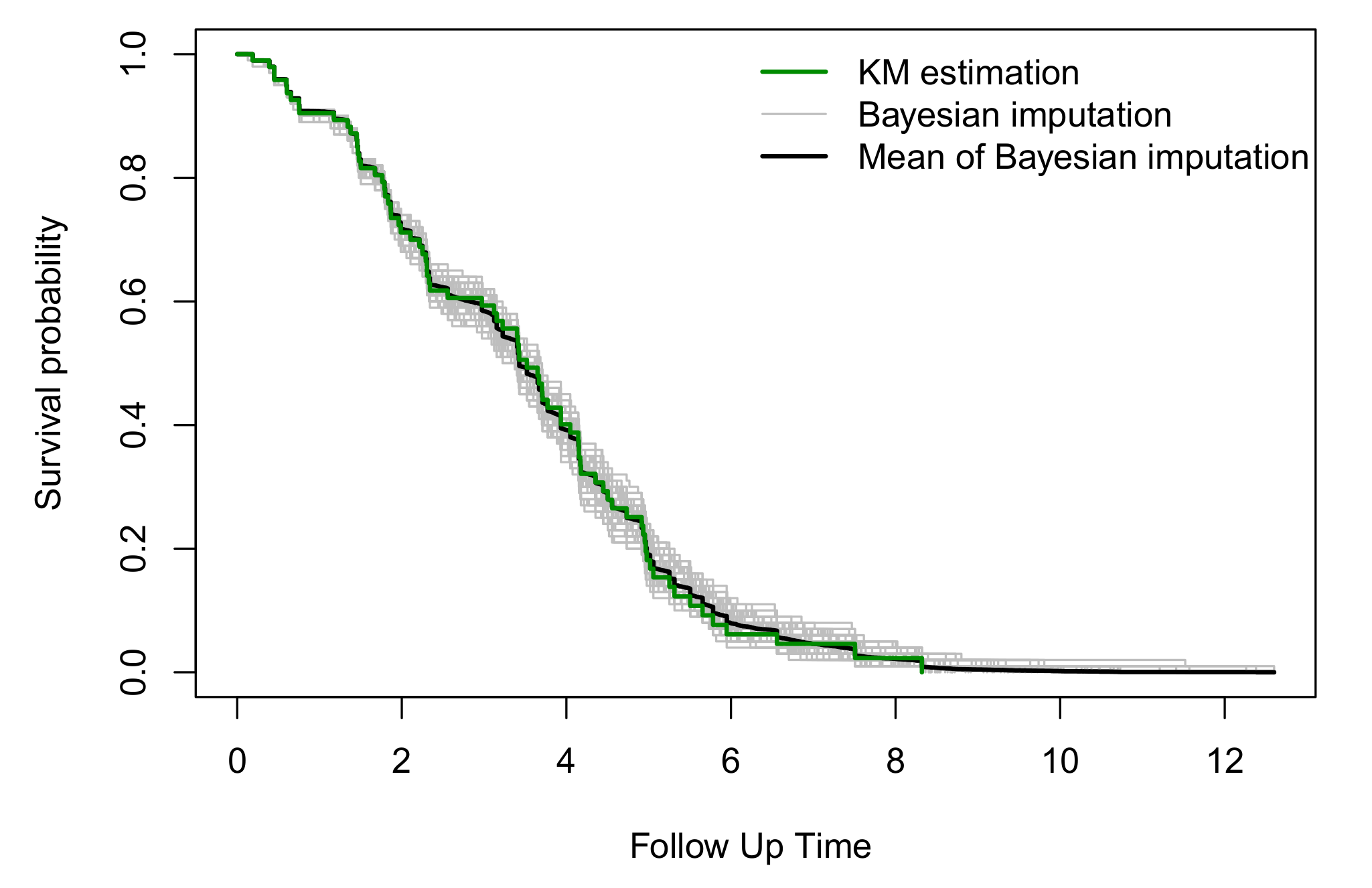
Rather than using only one single imputation as in Figure 1, we imputed the censored observations multiple times using the parametric Bayesian approach. Figure 2 compares the Kaplan–Meier estimation of the censored data with the Kaplan–Meier estimates from one hundred imputations using the parametric Bayesian approach. Figure 2 suggests that the Kaplan–Meier plots for all of the one hundred imputations are around the Kaplan–Meier estimate of the data, and as is expected, the mean of these one hundred Kaplan–Meier plots is a good approximation of the Kaplan–Meier estimate using the data before imputation.

By using the complete dataset after imputation, classical graphics, such as boxplots can be drawn. Figure 3 shows the boxplot for thirty imputed datasets comparing them to the true-failure times and the dataset omitting the censored values. It can be seen that the ranges of most of the imputation boxplots are near the range of true-failure times. Furthermore, medians are near to the true median of the data. This Figure shows that the distribution of data may not be sensitive to different imputations, however some extreme values may be imputed, as noted by Royston [13].

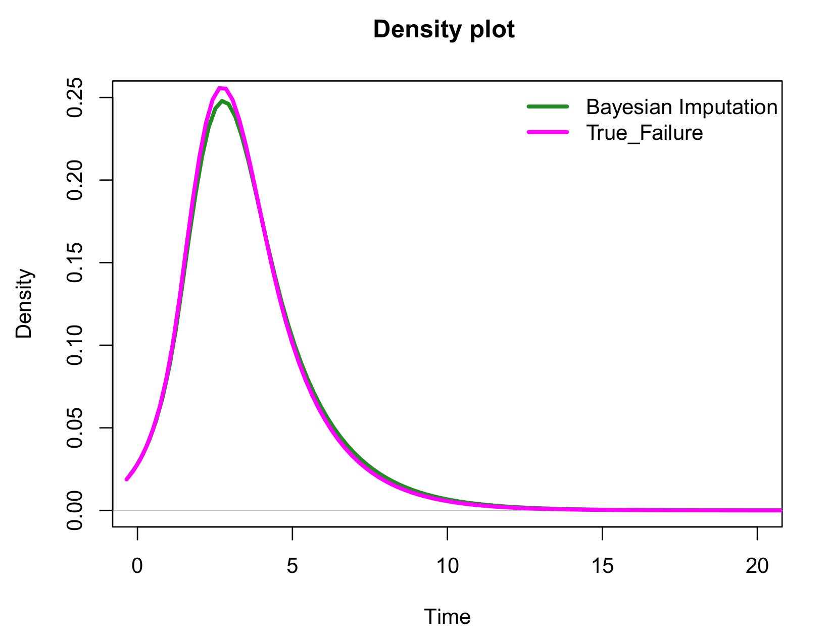
One of the aims of this paper is to impute the censored observations to enable plots of the density of the complete dataset as an additional visualizing tool to complement the common Kaplan–Meier plot. Figure 4 compares the density of the true-failure data to the density of the imputed dataset based on one single imputation. It is shown that the density plots are in general close to each other. The estimated density function is approximated by a polynomial spline using the logspline() function [24] in R.

The parametric Bayesian approach presented in this section could be extended to other survival distributions by changing the assumed distribution of the data and also the prior distributions.

3. Simulation Study

The primary purpose of this simulation study is to understand if the proposed imputation methods create accurate complete (imputed) datasets. The benefit of using simulated data, especially for examples that include censoring, is that we know not only the true underlying density function from which the data were generated from, but also the actual event time for each observation before censoring was applied. The study considers different percentages of random right censoring and also situations with decreasing, increasing and constant hazard functions.

In general, for any failure distribution $F\left(t\right)$ with survivor function $S\left(t\right)$ and for any censored density g(c) the exact amount of censoring is calculated as follows:

$$p={\int }_0^{\infty }S\left(c\right)g\left(c\right)dc$$

(9)

where the exponential distribution is assumed for the censored observations. Consequently, to achieve the desired percentage of censoring, the parameter of the exponential distribution needs to be calculated. Let p be a given percentage of censoring and assume that failure times follow a Weibull distribution with parameters $\alpha$ and $\lambda$ and that censored times follow exponential distribution with parameter $\beta$. So, by changing the percentage of censoring, the parameter of the censored distribution $\beta$ will change, as given by (10).

$$p=p(C<T)={\int }_0^{\infty }{\int }_c^{\infty }\alpha \lambda t^{\alpha -1}{e}^{-\lambda t^{\alpha }}\beta e^{-\beta c}dtdc={\int }_0^{\infty }{e}^{-\lambda c^{\alpha }}\beta e^{-\beta c}dc$$

(10)

The simulation procedure has the following steps:

• Sample survival times were generated from a desired distribution (here the samples are simulated from a Weibull distribution).
• Some observations are then assigned as censored values by:

  (a)

  Drawing random values from the censoring distribution, taken here to be an exponential distribution.

  (b)

  If the value that is generated from the censoring distribution is smaller than the actual survival value in the sample, then that individual is assumed to be censored with the censoring value obtained from the exponential distribution.

  (c)

  Otherwise the observation is uncensored with its generated survival time.

• The parametric Bayesian imputation method is used to impute values for the incomplete censored observations.
• Imputed values are combined together with the uncensored failure times to create a complete data set.

As the sample size may affect the imputation results, we consider the effects of three different sample sizes, namely small $(n=50)$, medium $(n=100)$, and large $(n=200)$. The percentage of censoring, as well as the sample size, will also have an impact in analysing survival data and also on any imputation. In the presence of a high percentage of censoring the variation in imputations may be increased. To study this, samples are generated using different percentages of censoring: low $(p=10\%)$, medium $(p=20\%)$ and high $(p=50\%)$. Furthermore, we want to investigate if there are any differences in the imputation results for samples from Weibull distributions with different hazard shapes. Hence, the data are simulated from constant, increasing, and decreasing hazards to see the impact, if any, on the performance of imputation.

The general procedure is as follows:

• A sample is generated from a particular Weibull distribution and the resulting values are considered as the true failure times.
• The desired percentage of censoring is applied, where for the censored observations the true failure values are replaced with values from an exponential distribution.
• Winbugs is used to fit the parametric Bayesian model and simulated draws of the imputed values for the censored observations are generated.
• Using 100 sets of these simulated imputed values and combining them with the uncensored event times, 100 complete datasets are generated.
• The difference between the survivor function based on the true values from the Weibull distribution and the survivor function based on the completed (imputed) datasets is calculated over a range of different time points.

The main goal is to show that our method is at least as good as the Kaplan–Meier estimate, so it is sensible to compare our results to Kaplan–Meier estimates. Consequently, as a visual measure to see how well the model is working, these 100 completed datasets are also compared to the range and interquartile range of the Kaplan–Meier estimates. If the difference between the true failures and our completed dataset are within these bounds for each of the 100 sets of data, it could be concluded that our method is comparable to the Kaplan–Meier estimates. The steps for plotting the bound and interquartile ranges are as follows:

• A total of 100 sets of data with the desired sample size are simulated from the specific Weibull distribution with no censoring.
• The survivor curve of these data is estimated using a Kaplan–Meier estimator.
• The Kaplan–Meier estimated value for all of the 100 simulation sets is subtracted from the true value of the Weibull distribution survivor function at specific time points.
• The maximum, minimum and quartiles of these differences are used to define a bound range and interquartile range over the time period of interest.

We will start with the simplest constant hazard scenario. The Weibull distribution has the constant hazard when $\alpha =1$ and it then reduces to an exponential distribution. In Figure 5 the results are shown for different sample sizes and different percentages of censoring where the samples are simulated from a $Weibull(1,4)$ distribution.

As it can be seen from Figure 5, the variability decreases and the bounds become tighter by increasing the sample size as is to be expected. The medians of the boxplot at each time point are nearly zero, and the boxplots are symmetric around the zero line. For samples of the same size, increasing the percentage of censoring causes some of the iterations to stay outside the bound, which means it is better not to use imputation methods when there is a high percentage of censoring.

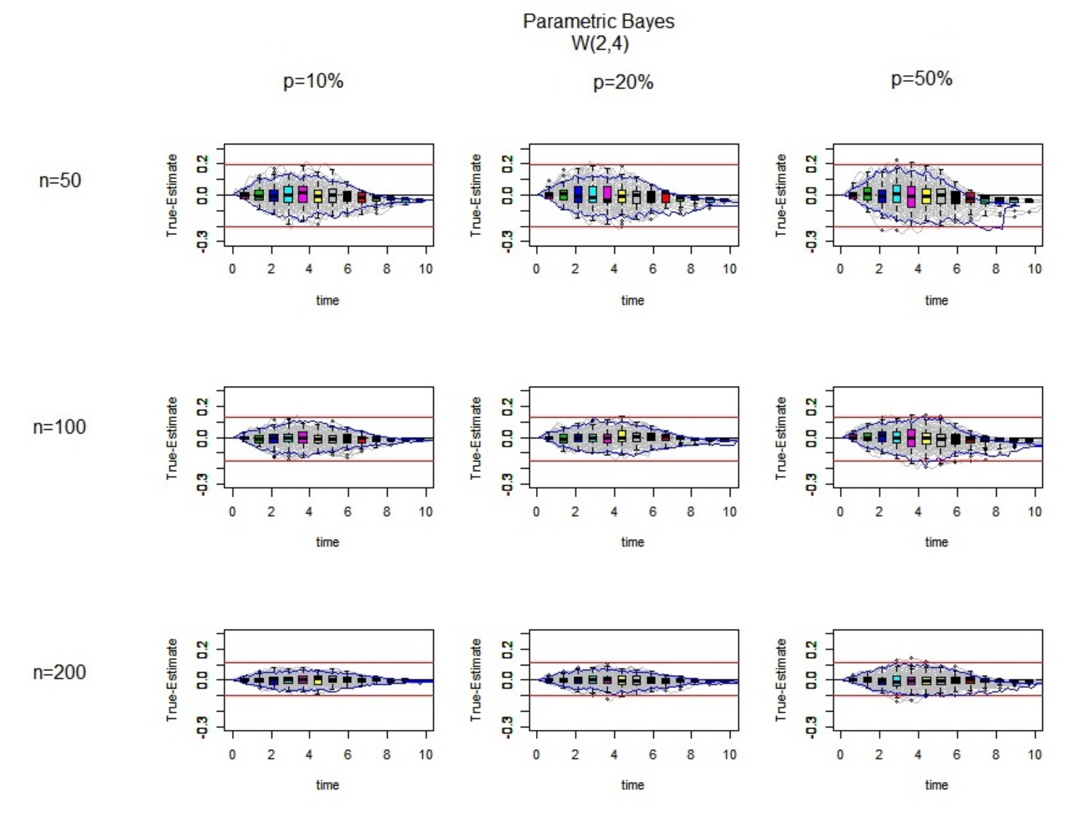
In the second simulation study, the data are simulated from a Weibull with $\alpha >1$ which leads to an increasing hazard situation.

As can be seen in Figure 6, by increasing the sample size, the imputations look reasonable as the difference between the true failure and Kaplan–Meier estimates for the 100 complete datasets are symmetrical around the zero line. However, at the later time points all of the iterations are below the zero line in nearly all of the graphs, which means that there is overestimation for the large censored values and this becomes worse when there is a high percentage of censoring.

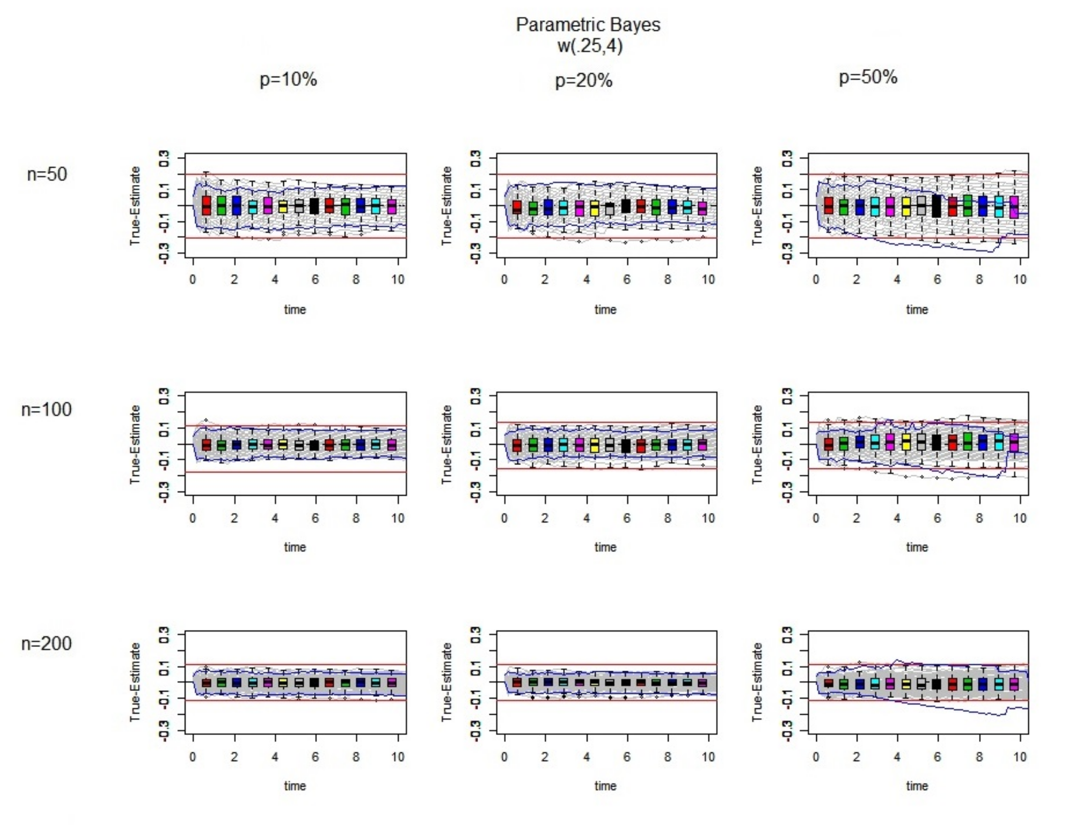
Finally, we consider a Weibull distribution with decreasing hazard ($\alpha <1$).

In Figure 7, as in Figure 5 and Figure 6, by increasing the sample size, the imputed values becomes closer to the true values. Moreover, in comparison to the increasing hazard case, at the later time points, the differences between the true failure and Kaplan–Meier estimates are still symmetric around the zero line, which means there is no significant under or over estimation of the censored observations. Moreover, the boxplots are symmetric with medians near zero lines in nearly all of the combinations of sample size and censoring.

In conclusion, there are some common features in all of the three situations considered, with increasing, decreasing and constant hazards. First, by increasing the sample size, the imputed values become closer to the true values. Second, we obtain reasonable imputed values when there is a low degree of censoring. Third, all of the 27 combinations were within the Kaplan–Meier bound, which means our parametric Bayesian approach is within the variability expected for the Kaplan–Meier estimate. However, across the different hazard scenarios, the imputed values seem more reliable in the case of decreasing or constant hazards, as nearly all of the iterations are placed symmetrically around the zero line, in contrast to the increasing hazard case where there is an indication of overestimation for large censored times.

4. Applications

The simulation study gave an insight into the likely performance of the proposed parametric Bayesian imputation methods. Building on these results, the proposed method is applied to two example datasets to illustrate the benefits of considering the parametric Bayesian method for imputing censored observations in time to event studies.

4.1. 6-MP Data

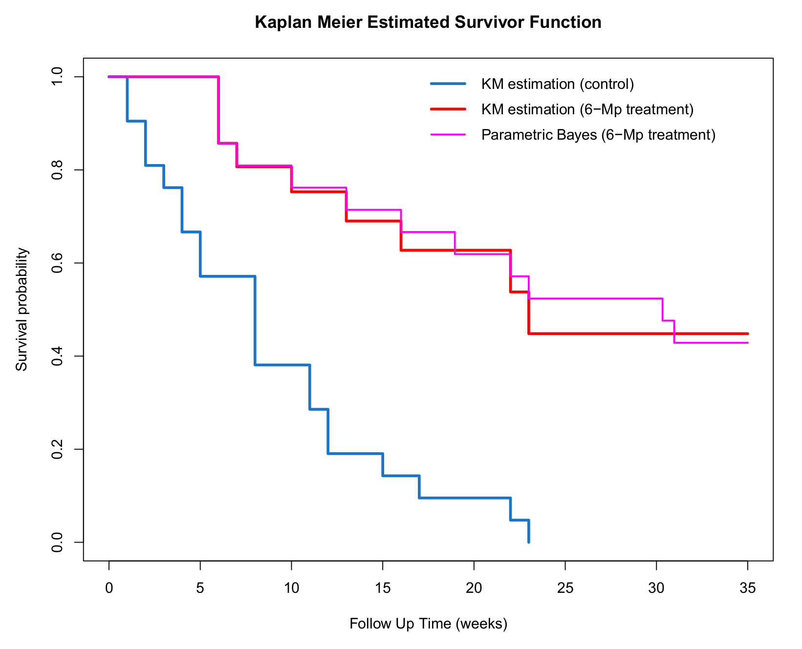
The first dataset is from the historical 6-MP trial. This dataset has been widely used in the survival analysis literature as an illustrative example in theoretical and applied work. The data are from a prospective clinical trial where 6-mercaptopurine (6-MP) was compared to a placebo in the maintenance of remission in acute leukaemia. (Gehan [25]; Freireich et al. [26]). The study was confined to patients under 20 years of age who had received no chemotherapy before admission. The first patient was enrolled in April 1959, and the last patient was entered in the study in April 1960. In the study, there are 42 leukaemia patients where 21 patients were allocated to a 6-MP treatment group and 21 to a control (placebo) group. The variable of interest is the time spent in remission. Some remission durations were censored due to loss to follow-up, and that many patients were alive with no recurrence of disease at the end of the study. There is no censoring in the control group; therefore, all of the graphical plots, including a density plot could be used as a visualising tool to summarise time in remission for the control group. In the treatment group, which contained 21 subjects, there are 12 censored observations i.e., more than half of the data. As a consequence, a plot of the estimated survivor function using the Kaplan–Meier estimator is the typical graphical summary used to compare the time to remission between those receiving the treatment and the controls.

The approach taken here is to impute the censored observations in the treatment group using the parametric Bayesian technique and provide a plot of the estimated density function as a useful complement to the Kaplan–Meier plot.

A plot of the estimated survivor functions for the control and treatment groups is given in Figure 8 where the censored observations have been imputed using the parametric Bayesian method assuming a Weibull distribution. It is apparent that the time to remission is shorter (i.e., worse prognosis) for the control group as the corresponding survivor function lies below the treatment group. An estimate of the median time to re-occurrence for the intervention group is 23 weeks while the median time for the control group is 8 weeks, which is further evidence that the treatment is effective.

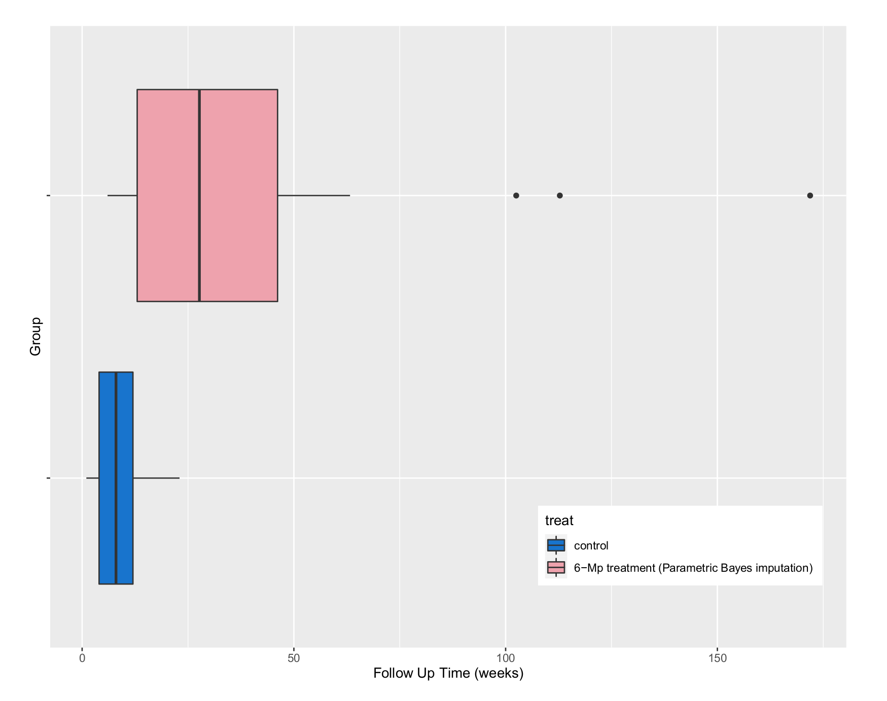
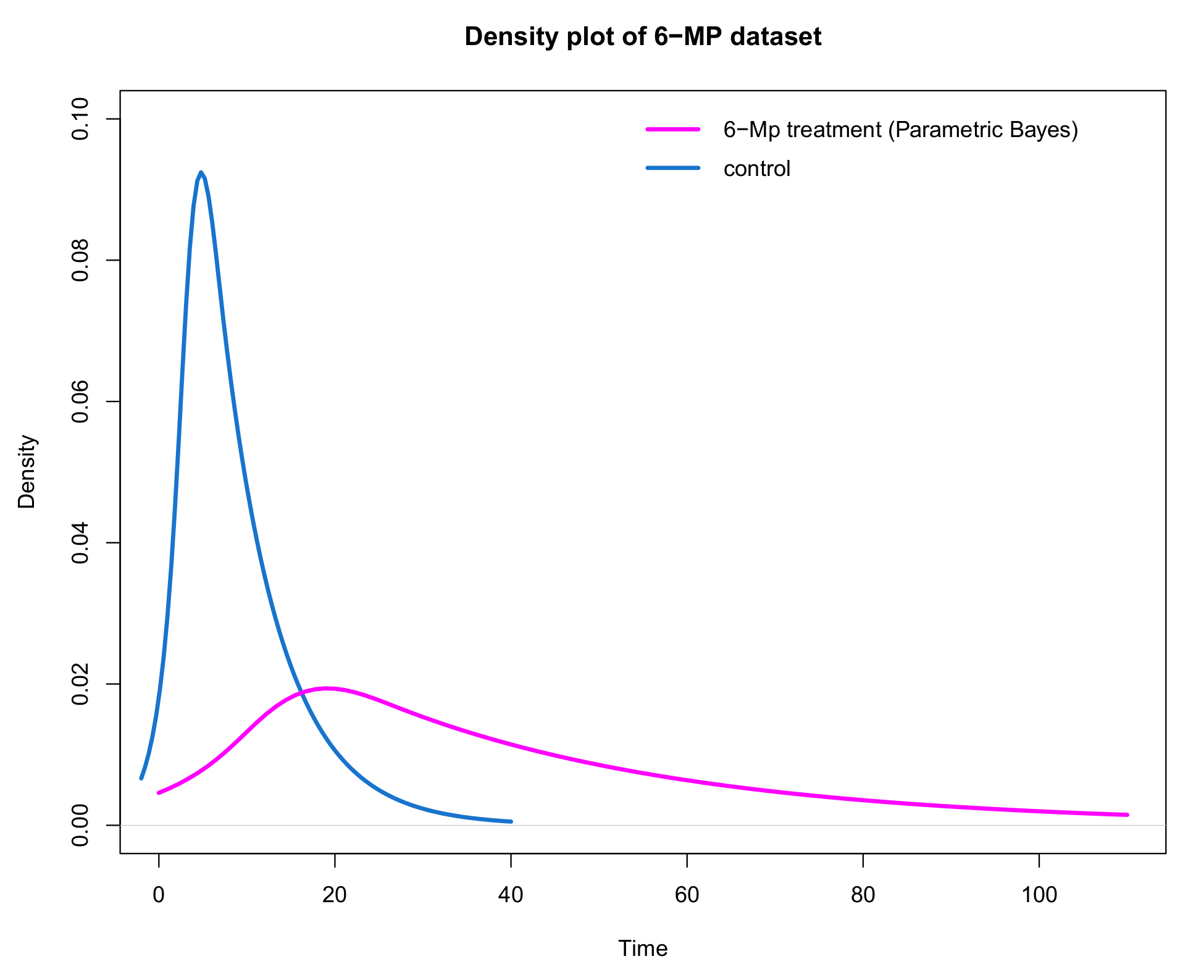
After imputation, a complete dataset is available allowing boxplots (Figure 9) and density plots (Figure 10) of time to recurrence for treatment and control groups to be generated. In particular, Figure 9 displays a boxplot of the time to recurrence by the treatment group while Figure 10 provides a density plot using the ‘complete’ data. The estimated density function is approximated by a polynomial spline [24].

It could be argued that these plots may be more informative when summarising the effect of treatment in units of time. For example, the underlying distribution for time to re-occurrence for the controls is right skewed with an estimated mean of 8.6 weeks with a minimum of 1 and a maximum of 23 and a standard deviation of 6.46. The plot of the distribution of remission times for those receiving the treatment is shifted to the right (highlighting the treatment effect) with an estimated mean of 40.77 minimum of 6 and maximum of 171. The distribution is also right skewed with a larger standard deviation of 41.9 (compared to the controls) suggesting that considerably longer times to re-occurrence are plausible on treatment.

Rather than providing a point estimate of a parameter like a mean or median, a 95% tolerance interval (with 95% confidence) could be calculated (using an appropriate transformation or non-parametric approach to account for the skewed nature of the distribution) to provide a reference range for remission times. For example, the tolerance interval for the controls is $(1,23)$ and (6, 171) for those receiving the treatment suggesting that it is unlikely to see a control patient with a time to remission greater than 23 weeks.

In conclusion, based on Figure 9 and Figure 10, the treatment appears more effective than the control as the distribution of time to re-occurrence is shifted in the positive direction with a heavier (right) tail suggesting that the ‘typical’ time to re-occurrence is greater for those on treatment with a possibility of a considerably longer time in remission compared to the controls. An individual in the control group is likely to have a remission time of between 1 and 23, while an individual on the 6-MP treatment is likely to have a remission time of between 6 and 171. However, based on the simulation results the imputed values for the censored observations might be less accurate due to the high percentage of censoring which needs to be considered when interpreting the results.

4.2. Bronchopulmonary Dysplasia (BPD) Data

The Bronchopulmonary Dysplasia (BPD) Data [27] provide a second illustration of the use of our imputation method. This dataset relates to low-birth weight newborns and the total number of hours needed on (oxygen) treatment for a chronic lung disorder to abate. Note that low values are associated with a good outcome. Infants were randomised into either a treatment (i.e., surfactant therapy) or a control group. There are two censored observations in the treatment group of 35 infants, and three censored observations in the control group of 43 infants.

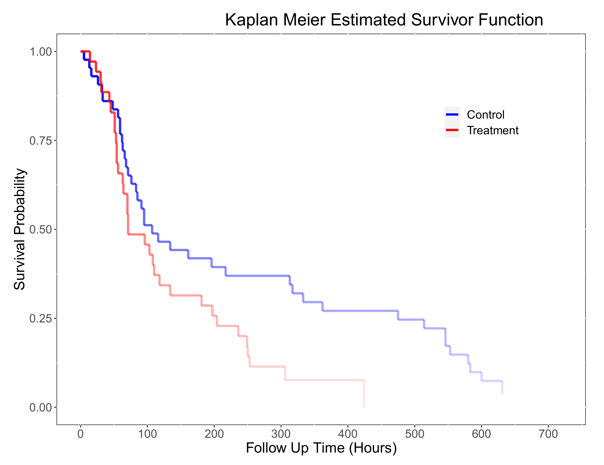
Figure 11 shows the alpha blending enhanced plot of the Kaplan–Meier estimation. Based on this plot, the estimated median number of hours on oxygen therapy for those infants who did not have surfactant therapy is 107 and the estimated median number of hours for those who had the therapy is 71, suggesting that surfactant is a beneficial therapy.

Although there are only a small number of censored observations in the dataset, ignoring them is not statistical best practice. Instead, censored observations in both groups were imputed using a parametric Bayesian approach. As the percentage of censored observations in both the treatment and control group is small, based on our simulation study the imputation results should be good estimates of their true unknown event times.

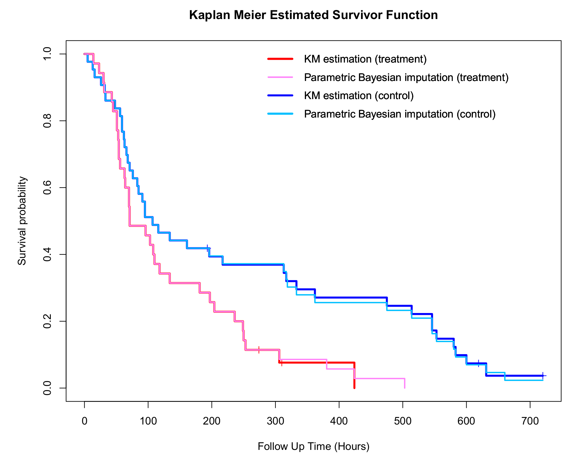
The Kaplan–Meier estimates of the survival function for the treatment and control groups, along with the corresponding ones using imputation, are shown in Figure 12. The assumed response distribution used in the parametric Bayesian imputation is the Weibull distribution.

Based on Figure 12, in both the treatment and control group, the survivor estimates of the “complete” dataset after imputation using parametric Bayesian method is in agreement with the Kaplan–Meier estimate before imputation, which is as expected as there are only a small number of censored observations in each group. The boxplot of the completed datasets is shown in Figure 13 where the treatment effect is quite evident.

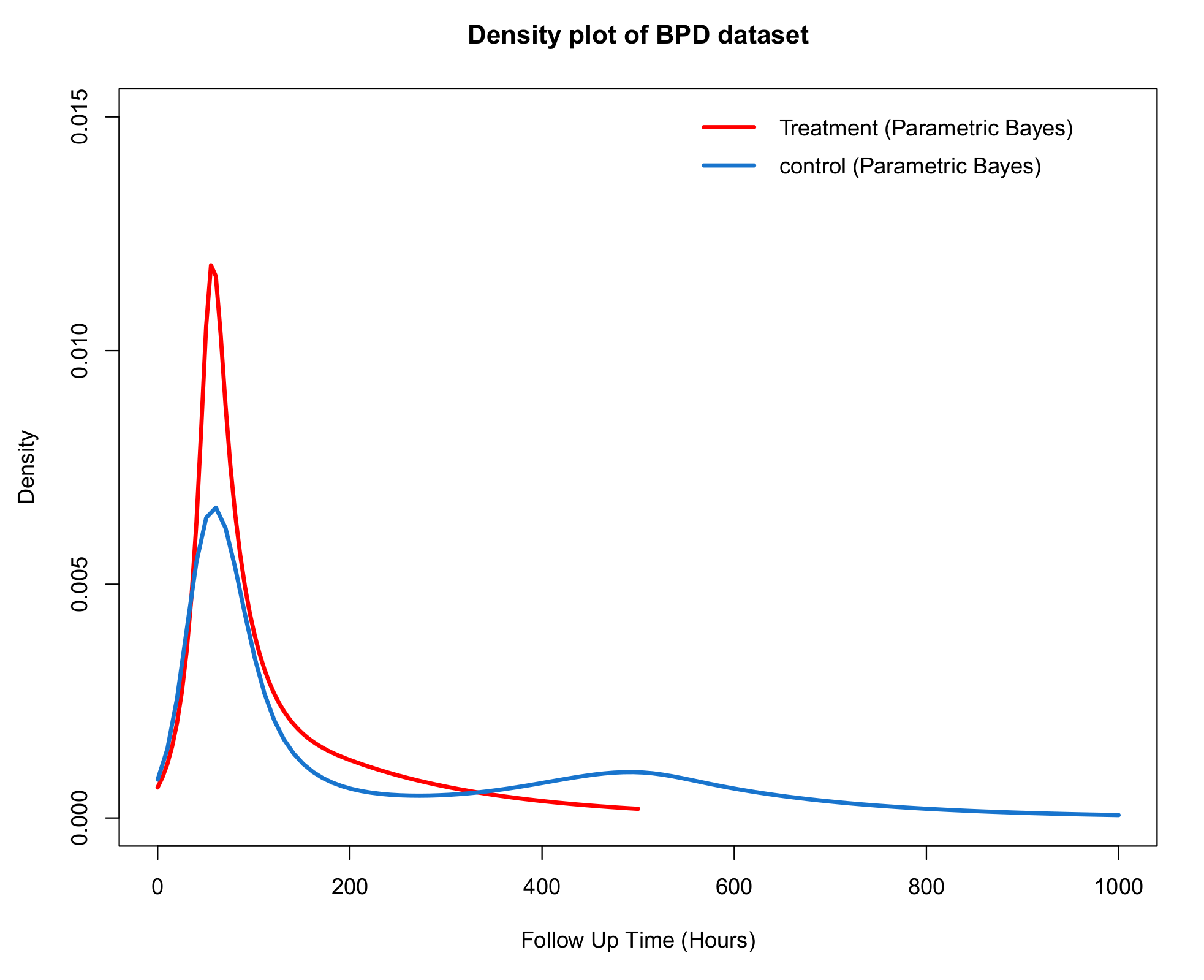
The density plot using a polynomial spline is shown in Figure 14. The densities look quite similar initially while a separation occurs beyond 100 h. Here, the effect of treatment becomes more evident with the distribution of the time to come off treatment with a shorter tail than for the control group.

In summary, from Figure 11, Figure 13 and Figure 14 it is clear that surfactant therapy plays an important role in reducing the number of hours of oxygen therapy required among low birth weight infants who require treatment. A possible explanation for the results seen in the density plot is that there are two subgroups of infants, those who will recover quickly, for whom there is no real treatment effect, and a second group of sicker infants where the additional surfactant treatment is effective in reducing the time required on oxygen therapy.

5. Discussion

The main aim of this paper was to consider censored data as a form of missing, incomplete, data and to propose a parametric Bayesian approach to impute these partially observed values. Whether the imputed values are good estimates of the true unknown values depends on assumptions about homogeneity of the groups; it assumes that the censored values are not explicitly different from the observed ones. In this paper, the imputed values of censored observations were used to produce more interpretable graphical summaries of time-to-event data, such as a density plot, which may usefully complement Kaplan–Meier plots. The imputation approach is intended to be used for the visual exploration and presentation of survival data and give a simple, interpretable display for physicians and patients to better understand summaries generated from time to event studies. The parametric Bayesian approach is computationally fast, taking seconds to one minute to run depending on the percentages of censoring.

To study the performance of our approach we carried out a simulation study, using a parametric Bayesian approach to impute the censored observations. The simulation study results were obtained for differing sample sizes and percentages of censoring.

Based on our simulation results, if the sample size is large enough (for example greater than a hundred) and also in the presence of at most a moderate percentage of censoring (not more than twenty percent), the parametric Bayesian imputation method works quite well when estimating a survivor function and is comparable to the Kaplan–Meier estimator. As the sample size increased the imputed values became more accurate, but for a given sample size becomes less so, as the proportion of censoring increases. In general, this imputation method is not recommended when a high percentage of censoring is present, as when half or more of the data are censored there is insufficient information in the observed failure times to provide meaningful imputations.

The examples are based on the Weibull model but the methods could be extended to other survival distributions and other Bayesian survival models by changing the assumed distribution of the data and using an appropriate prior distributions. The model could also be extended to the incorporate baseline covariate. In the case that there is no recognisable and analytically tractable prior, MCMC methods can be used to draw from the posterior and predictive distributions.

The purpose of this paper is to demonstrate the idea of Bayesian imputation and the feasibility and usefulness of this approach. Other work on using more flexible non-parametric Bayesian frameworks and also investigating the sensitivity to the choice of distribution will be reported in a subsequent paper.

References

1. Gould, S.J. The median isn’t the message. Discover 1985, 6, 40–42. [Google Scholar] [CrossRef] [Green Version]
2. Jalali, A.; Alvarez-Iglesias, A.; Roshan, D.; Newell, J. Visualising statistical models using dynamic nomograms. PLoS ONE 2019, 14, e0225253. [Google Scholar] [CrossRef] [PubMed]
3. Wei, G.C.; Tanner, M.A. Posterior computations for censored regression data. J. Am. Stat. Assoc. 1990, 85, 829–839. [Google Scholar] [CrossRef]
4. Wei, G.C.; Tanner, M.A. Applications of multiple imputation to the analysis of censored regression data. Biometrics 1991, 47, 1297–1309. [Google Scholar] [CrossRef]
5. Pan, W.; Connett, J.E. A multiple imputation approach to linear regression with clustered censored data. Lifetime Data Anal. 2001, 7, 111–123. [Google Scholar] [CrossRef]
6. Ageel, M. A novel means of estimating quantiles for 2-parameter Weibull distribution under the right random censoring model. J. Comput. Appl. Math. 2002, 149, 373–380. [Google Scholar] [CrossRef] [Green Version]
7. Chiou, K.C. A Study of Imputing Censored Observations for 2-Parameter Weibull Distribution Based on Random Censoring; Department of Accounting and Statistics, The Overseas Chinese Institute of Technology: Taichung, Taiwan, 2003; pp. 1–5. [Google Scholar]
8. Cantor, A. Imputation for Censored Observations in Survival Studies Allowing for a Positive Cure Rate; University of Alabama at Birmingham: Birmingham, AL, USA, 2009. [Google Scholar]
9. Lue, H.H.; Chen, C.H.; Chang, W.H. Dimension reduction in survival regressions with censored data via an imputed spline approach. Biom. J. 2011, 53, 426–443. [Google Scholar] [CrossRef]
10. Buckley, J.; James, I. Linear regression with censored data. Biometrika 1979, 66, 429–436. [Google Scholar] [CrossRef]
11. Jackson, D.; White, I.R.; Seaman, S.; Evans, H.; Baisley, K.; Carpenter, J. Relaxing the independent censoring assumption in the Cox proportional hazards model using multiple imputation. Stat. Med. 2014, 33, 4681–4694. [Google Scholar] [CrossRef] [Green Version]
12. Royston, P. The lognormal distribution as a model for survival time in cancer, with an emphasis on prognostic factors. Stat. Neerl. 2001, 55, 89–104. [Google Scholar] [CrossRef]
13. Royston, P.; Parmar, M.K.; Altman, D.G. Visualizing length of survival in time-to-event studies: A complement to Kaplan–Meier plots. J. Natl. Cancer Inst. 2008, 100, 92–97. [Google Scholar] [CrossRef] [PubMed] [Green Version]
14. Taylor, J.M.; Murray, S.; Hsu, C.H. Survival estimation and testing via multiple imputation. Stat. Probab. Lett. 2002, 58, 221–232. [Google Scholar] [CrossRef]
15. Faucett, C.L.; Schenker, N.; Taylor, J.M. Survival analysis using auxiliary variables via multiple imputation, with application to AIDS clinical trial data. Biometrics 2002, 58, 37–47. [Google Scholar] [CrossRef] [PubMed]
16. Hsu, C.H.; Taylor, J.M.; Murray, S.; Commenges, D. Survival analysis using auxiliary variables via non-parametric multiple imputation. Stat. Med. 2006, 25, 3503–3517. [Google Scholar] [CrossRef]
17. Hsu, C.H.; Taylor, J.M. Nonparametric comparison of two survival functions with dependent censoring via nonparametric multiple imputation. Stat. Med. 2009, 28, 462–475. [Google Scholar] [CrossRef] [Green Version]
18. Hsu, C.H.; Taylor, J.M.; Hu, C. Analysis of accelerated failure time data with dependent censoring using auxiliary variables via nonparametric multiple imputation. Stat. Med. 2015, 34, 2768–2780. [Google Scholar] [CrossRef] [Green Version]
19. Ibrahim, J.G.; Chen, M.H.; Sinha, D. Bayesian Survival Analysis; Wiley Online Library: Hoboken, NJ, USA, 2005. [Google Scholar]
20. Gelf, A.E.; Smith, A.F. Sampling-based approaches to calculating marginal densities. J. Am. Stat. Assoc. 1990, 85, 398–409. [Google Scholar]
21. Lunn, D.; Jackson, C.; Best, N.; Thomas, A.; Spiegelhalter, D. The BUGS Book: A Practical Introduction to Bayesian Analysis; CRC Press: Boca Raton, FL, USA, 2012. [Google Scholar]
22. Christensen, R.; Johnson, W.; Branscum, A.; Hanson, T.E. Bayesian Ideas and Data Analysis: An Introduction for Scientists and Statisticians; CRC Press: Boca Raton, FL, USA, 2011. [Google Scholar]
23. Halabi, S.; Singh, B. Sample size determination for comparing several survival curves with unequal allocations. Stat. Med. 2004, 23, 1793–1815. [Google Scholar] [CrossRef]
24. Kooperberg, C. Logspline: Logspline Density Estimation Routines. 2016. Available online: https://CRAN.R-project.org/package=logspline (accessed on 1 February 2018).
25. Gehan, E.A. A generalized Wilcoxon test for comparing arbitrarily singly-censored samples. Biometrika 1965, 52, 203–224. [Google Scholar] [CrossRef]
26. Acute Leukemia Group B; Freireich, E.J.; Gehan, E.; Frei, E.M., III; Schroeder, L.R.; Wolman, I.J.; Anbari, R.; Burgert, E.O.; Mills, S.D.; Pinkel, D.; et al. The effect of 6-mercaptopurine on the duration of steroid-induced remissions in acute leukemia: A model for evaluation of other potentially useful therapy. Blood 1963, 21, 699–716. [Google Scholar]
27. Hosmer, D.W.; Lemeshow, S.; May, S. Applied Survival Analysis: Regression Modeling of Time-to-Event Data, 2nd ed.; Wiley-Interscience: Hoboken, NJ, USA, 2008. [Google Scholar]
28. Sturtz, S.; Ligges, U.; Gelman, A. R2WinBUGS: A Package for Running WinBUGS from R. J. Stat. Softw. 2005, 12, 1–16. [Google Scholar] [CrossRef] [Green Version]
Figure 1. The Kaplan–Meier survivor plots: for the full data with censoring; the true failure times; omitting censored observations; and using parametric Bayesian imputation for the censored values.
Stats 05 00006 g001
Figure 2. Kaplan–Meier plots of the censored data compared with the mean of the Kaplan–Meier estimates from one hundred imputations using a parametric Bayesian approach.
Stats 05 00006 g002
Figure 3. Boxplots of the true failure times and when omitting censored observations compared to the 30 draws of parametric Bayesian imputations.
Stats 05 00006 g003
Figure 4. Comparing the density of the true-failure data to the density of the imputed dataset using a parametric Bayesian approach based on one single imputation.
Stats 05 00006 g004
Figure 5. The difference between the true values and the estimated ones (True-Estimate) (grey lines) using the parametric Bayesian approach for 100 datasets is presented. It is generated from W e i b u l l ( 1 , 4 ) using exponential censoring for different sample size and different percentage of censoring. In each individual panel, the red bound and the blues bound are the bound and interquartile range for the Kaplan–Meier estimates, respectively. Over the range of different time points, the boxplots of True-Estimate values are also plotted.
Stats 05 00006 g005
Figure 6. The difference between the true values and the estimated ones (True-Estimate) (grey lines) using the parametric Bayesian approach for 100 datasets is presented. It is generated from a W e i b u l l ( 2 , 4 ) using exponential censoring for different sample sizes and different percentages of censoring. In each individual panel, the red bound and the blues bound are the bound and interquartile range for the Kaplan–Meier estimates, respectively. Over range of different time points the boxplots of True-Estimate values are also plotted.
Stats 05 00006 g006
Figure 7. The difference between the true values and the estimated ones (True-Estimate) (grey lines) using the parametric Bayesian approach for 100 datasets is presented. It is generated from a W e i b u l l ( 0.25 , 4 ) using exponential censoring for different sample sizes and different percentages of censoring. In each individual panel, the red bound and the blues bound are the bound and interquartile range for the Kaplan–Meier estimates, respectively. Over a range of different time points, the boxplots of True-Estimate values are also plotted.
Stats 05 00006 g007
Figure 8. Kaplan–Meier plot for the complete dataset in the treatment group using s parametric Bayesian approach compared to the Kaplan–Meier of treatment and control group in the 6-MP dataset.
Stats 05 00006 g008
Figure 9. Comparing boxplots of time to re-occurrence in the control and treatment group using the parametric Bayesian imputation approach.
Stats 05 00006 g009
Figure 10. Comparing the density plot of control and treatment groups using the parametric Bayesian approach to impute censored observations in the treatment group.
Stats 05 00006 g010
Figure 11. Kaplan–Meier plot for treatment and control group in the BPD dataset using alpha blending on the lines to show how many patients are at risk at the time.
Stats 05 00006 g011
Figure 12. Kaplan–Meier plot for the complete dataset in the treatment and control group using parametric Bayesian approach compared to the Kaplan–Meier estimates for the original data.
Stats 05 00006 g012
Figure 13. Boxplots of the survival time for the control and treatment groups after imputing censored observations using the parametric Bayesian approach.
Stats 05 00006 g013
Figure 14. Comparing the density plot of the control and treatment group using the parametric Bayesian approach to impute censored observations in both groups.
Stats 05 00006 g014
Publisher’s Note: MDPI stays neutral with regard to jurisdictional claims in published maps and institutional affiliations.