The One Standard Error Rule for Model Selection: Does It Work?

Abstract

Previous research provided a lot of discussion on the selection of regularization parameters when it comes to the application of regularization methods for high-dimensional regression. The popular “One Standard Error Rule” (1se rule) used with cross validation (CV) is to select the most parsimonious model whose prediction error is not much worse than the minimum CV error. This paper examines the validity of the 1se rule from a theoretical angle and also studies its estimation accuracy and performances in applications of regression estimation and variable selection, particularly for Lasso in a regression framework. Our theoretical result shows that when a regression procedure produces the regression estimator converging relatively fast to the true regression function, the standard error estimation formula in the 1se rule is justified asymptotically. The numerical results show the following: 1. the 1se rule in general does not necessarily provide a good estimation for the intended standard deviation of the cross validation error. The estimation bias can be 50–100% upwards or downwards in various situations; 2. the results tend to support that 1se rule usually outperforms the regular CV in sparse variable selection and alleviates the over-selection tendency of Lasso; 3. in regression estimation or prediction, the 1se rule often performs worse. In addition, comparisons are made over two real data sets: Boston Housing Prices (large sample size n, small/moderate number of variables p) and Bardet–Biedl data (large p, small n). Data guided simulations are done to provide insight on the relative performances of the 1se rule and the regular CV.

1. Background

Resampling and subsampling methods were widely utilized in many statistical and machine learning applications. In high-dimensional regression learning, for instance, bootstrap and subsampling play important roles in model selection uncertainty quantification and other model selection diagnostics (see, e.g., [1] for references). Cross-validation (CV) (as a subsampling tool) and closely related methods were proposed to assess quality of variable selection performance in terms of F- and G-measures ([2]) and to determine variable importances ([3]).

In this paper, we focus on the examination of cross-validation as used for model selection. A core issue is how to properly quantify variabilities in subsamplings and associated evaluations, which is a really challenging issue that is yet to be solved, to the best of our knowledge. In application of variable and model selection, a popular practice is to use the “one standard error rule”. However, its validity hinges crucially on the goodness of the standard error formula used in the approach. Our aim in this work is to study the standard error estimation issue and its consequences on variable selection and regression estimation.

In this section, we provide a background on tuning parameter selection for high-dimensional regression.

1.1. Regularization Methods

Regularization methods are now widely used to tackle the problem of curse of dimensionality in high-dimensional regression analysis. By imposing a penalty on the complexity of the solution, it can solve an ill-posed problem or prevent overfitting. Examples include Lasso ([4]) and Ridge regression ([5,6]), which add an $l_1$ and $l_2$ penalty on the coefficient estimates, respectively, to the usual least-squares fit objective function.

Specifically, given a response vector $y\in {\mathbb{R}}^n$, a matrix $X\in {\mathbb{R}}^{n\times p}$ of predictor variables and a vector of intercept $\alpha$, the Lasso estimate is defined as

$${\widehat{\beta }}^{lasso}={\mathbf{argmin}}_{\beta \in {\mathbb{R}}^p}{\Vert y-\alpha -X\beta \Vert }_2^2+\lambda \sum _{j=1}^p\mid {\beta }_j\mid ,$$

(1)

and the ridge estimate is defined as

$${\widehat{\beta }}^{ridge}={\mathbf{argmin}}_{\beta \in {\mathbb{R}}^p}{\Vert y-\alpha -X\beta \Vert }_2^2+\lambda \sum _{j=1}^p{\beta }_j^2.$$

(2)

The tuning parameter $\lambda$ controls the strength of the penalty. As is well known, the nature of the ${\ell }_1$ penalty causes some coefficients to be shrunken to zero exactly while the ${\ell }_2$ penalty can shrink all of the coefficients towards zero, but it typically does not set any of them exactly to zero. Thus, an advantage of Lasso is that it makes the results simpler and more interpretable. In this work, ridge regression will be considered when regression estimation (i.e., the focus is on the accurate estimation of the regression function) or prediction is the goal.

1.2. Tuning Parameter Selection

The regularization parameter, or the tuning parameter, determines the extent of penalization. A traditional way to select a model is to use an information criterion such as Akaike information criterion (AIC) ([7,8]), Bayesian information criterion (BIC) and its extension ([9,10,11]). A more commonly used way for tuning parameter selection is the cross-validation ([12,13,14]). For recent work on cross-validation for consistent model selection for high-dimensional regression, see [15].

The idea of K-fold cross validation is to split the data into K roughly equal-sized parts: $F_1,\dots ,F_K$. For the k-th part where $k=1,2,\dots ,K$, we consider training on $(x_i,y_i),i\notin F_k$ and evaluation on $(x_i,y_i),i\in F_k$. For each value of the tuning parameter $\lambda \in \{{\lambda }_1,\dots ,{\lambda }_m\}$, a set of candidate values, we compute the estimate ${\widehat{f_{\lambda }}}^{(-k)}$ on the training set, and record the total error on the validation set:

$$C{V}_k\left(\lambda \right)=\sum _{i\in F_k}{(y_i-{\widehat{f_{\lambda }}}^{(-k)}\left(x_i\right))}^2.$$

(3)

For each tuning parameter value $\lambda$, we compute the average error over all folds:

$$CV\left(\lambda \right)=\frac{1}{K}\sum _{k=1}^{K}C{V}_k\left(\lambda \right).$$

(4)

We then choose the value of tuning parameter that minimizes the above average error,

$${\widehat{\lambda }}_{min}={\mathbf{argmin}}_{\lambda \in \{{\lambda }_1,\dots ,{\lambda }_m\}}CV\left(\lambda \right).$$

(5)

1.3. Goal for the One Standard Error Rule

The “one standard error rule” (1se rule) for model selection was first proposed for selecting the right sized tree ([16]). It is also suggested to pick the most parsimonious model within one standard error of the minimum cross validation error ([17]). Such a rule acknowledges the fact that the bias-variance trade-off curve is estimated with error, and hence takes a conservative approach: a smaller model is preferred when the prediction errors are more or less indistinguishable. To estimate the standard deviation of $CV\left(\lambda \right)$ at each $\lambda \in \{{\lambda }_1,\dots ,{\lambda }_m\}$, one computes the sample standard deviation of validation errors in $C{V}_1\left(\lambda \right),\dots ,$ $C{V}_K\left(\lambda \right)$:

$$SD\left(\lambda \right)=\sqrt{Var(C{V}_1\left(\lambda \right),\dots ,C{V}_K\left(\lambda \right))}.$$

(6)

Then, we estimate the standard deviation of $CV\left(\lambda \right)$, which is declared the standard error of $CV\left(\lambda \right)$, by

$$SE\left(\lambda \right)=SD\left(\lambda \right)/\sqrt{K}.$$

(7)

The organization of the rest of the paper is as follows. Section 2 examines validity of the 1se rule from a theoretical perspective. Section 3 describes the objectives and approaches of our numerical investigations. Section 4 presents the experimental results of the 1se rule in three different aspects. Section 5 applies the 1se rule on two real data sets and examine its performances via data guided simulations. Section 6 concludes the paper. Appendix A gives additional numerical results and Appendix B provides the proof of the main theorem in the paper.

2. Theoretical Result on the One-Standard-Error Rule

2.1. When Is the Standard Error Formula Valid?

The 1se rule makes intuitive sense, but its validity is not clear at all. The issue is that the $CV$ errors completed at different folds are not independent, which invalidates the standard error formula for the sample mean of i.i.d. observations. Note that the validity of the standard error is equivalent to the validity of the sample standard deviation expressed in Equation (6). Thus, it suffices to study if and to what extent the usual sample variance properly estimates the targeted theoretical variance.

In this section, we investigate the legitimacy of the standard error formula for a general learning procedure. We focus on the regression case, but similar results hold for classification as well.

Let $\delta$ be a learning procedure that produces the regression estimator ${\widehat{f}}_{\delta }(x;{\mathbb{D}}^n)$ based on the data ${\mathbb{D}}^n={(x_i,y_i)}_{i=1}^n$. Throughout the section, we assume K is given and for simplicity, n is a multiple of K. Define $C{V}_k\left(\delta \right)={\sum }_{i\in F_k}{(y_i-{\widehat{f}}_{\delta }(x_i;{\mathbb{D}}_{(-k)}^n))}^2$, where ${\mathbb{D}}_{(-k)}^n$ denote the observations in ${\mathbb{D}}^n$ that do not belong to $F_k$ and $k=1,2,\dots ,K$.

The $SE$ of the $CV$ errors of the learning procedure $\delta$ is defined as

$$SE\left(\delta \right)=\sqrt{\frac{\frac{1}{K-1}{\sum }_{k=1}^K{\left(C{V}_k\left(\delta \right)-\frac{1}{K}{\sum }_{k=1}^{K}C{V}_k\left(\delta \right)\right)}^2}{K}}.$$

To study the $SE$ formula, given that K is fixed, it is basically equivalent to studying the sample variance formula, i.e.,

$${\mathbb{S}}_n\left(\delta \right)=\frac{1}{K-1}\sum _{k=1}^K{(C{V}_k\left(\delta \right)-\frac{1}{K}\sum _{k=1}^{K}C{V}_k\left(\delta \right))}^2.$$

The validity of these formulas (in an asymptotic sense) hinges on that the correlation between $C{V}_{k_1}\left(\delta \right)$ and $C{V}_{k_2}\left(\delta \right)$ for $k_1\ne k_2$ approaches zero as $n\to \infty$.

Definition 1.

The sample variance ${\mathbb{S}}_n\left(\delta \right)$ is said to be asymptotically relatively unbiased (ARU) if

$$\frac{\mathbb{E}{\mathbb{S}}_n\left(\delta \right)-Var\left(C{V}_k\left(\delta \right)\right)}{Var\left(C{V}_k\left(\delta \right)\right)}\to 0$$

as $n\to \infty$.

Clearly, if the property above holds, the $SE$ formula is properly justified in terms of the relative estimation bias being negligible. Then, the 1se rule is sensible.

For $p>0$, define the $L_p$-norm

$$\left|\right|f\left|\right|={\left(\int f^p\left(x\right)P_X\left(dx\right)\right)}^{1/p},$$

where $P_X$ denotes the probability distribution of X from which $X_1,X_2,\dots ,X_n$ are drawn. Let ${\widehat{f}}_{\delta ,n}$ denote the estimator ${\widehat{f}}_{\delta }(x;{\mathbb{D}}^n)$.

Theorem 1.

If $\mathbb{E}\left(\right||f-{\widehat{f}}_{\delta ,n}{\left|\right|}_4^4)=o\left(\frac{1}{n}\right)$, then ${\mathbb{S}}_n\left(\delta \right)$ is asymptotically relatively unbiased.

Remark 1.

The condition $\mathbb{E}\left(\right||f-{\widehat{f}}_{\delta ,n}{\left|\right|}_4^4)=o\left(\frac{1}{n}\right)$ holds if the regression procedure is based on a parametric model under regularity conditions. For instance, if we consider a linear model with $p_0$ terms, then under sensible conditions (e.g., [15], p. 111), $E\left(\right||f-{\widehat{f}}_{\delta ,n}{\left|\right|}^4)=\mathcal{O}\left(\frac{p_0^2}{n^2}\right)$ and consequently as long as $p_0=o\left(\sqrt{n}\right)$, the variance estimator ${\mathbb{S}}_n\left(\delta \right)$ is asymptotically relatively unbiased.

Remark 2.

The above result suggests that when relatively simple models are considered, the 1se rule may be reasonably applicable. In the same spirit, when sparsity oriented variable selection methods are considered as candidate learning methods, if the most relevant selected models are quite sparse, the 1se rule may be proper.

2.2. An Illustrative Example

Our theorem shows that the standard error formula is asymptotically valid when the correlation between the $CV$ errors at different folds is relatively small, which is related to the rate of convergence of the regression procedure. In this section, we illustrate how the dependence affects the validity of the standard error formula in a concrete example. For ease in highlighting the dependence among the $CV$ errors at different folds, we consider a really simple setting, where the true regression function is a constant. The simplicity allows us to calculate the variance and covariance of the $CV$ errors explicitly and then see the essence. The insight gained, however, is more broadly applicable.

The true data generating model is $Y=\theta +ϵ$, where $\theta \in R$ is unknown. Given data ${\mathbb{D}}^n$, for an integer r as a factor of n, the regression procedure considers only the first, r-th, $\left(2r\right)$-th, ..., $(n/r)$-th observations and take the corresponding sample mean of Y to estimate $f\left(x\right)=0$.

Suppose $l=\frac{n}{Kr}$ is an integer. Then, when applying the K-fold $CV$, the training sample size is $(K-1)\frac{n}{K}$ but only $(K-1)l$ observations are actually used to estimate f. Let $W_i$, $W_j$ denote the $CV$ errors on the i-th and j-th fold, $1\le i,j\le K$. Then, it can be shown that

$$Var\left(W_i\right)\asymp n(1+\frac{n}{l^2})$$

(8)

and

$$Cov(W_i,W_j)\asymp \frac{n^2}{l^2}$$

(9)

for $i\ne j$, where ≍ denotes the same order.

Therefore, the standard error formula is ARU if and only if $\frac{l}{\sqrt{n}}\to \infty$.

In this illustrating example, when l is small (recall that only l observations are used in each fold for training), the regression estimator obtained from excluding one fold respectively are highly dependent, which makes the sample variance formula problematic. In contrast, when l is large, e.g., $l=\frac{n}{K}$ (i.e., all the observations are used), the dependence of the $CV$ errors at different folds becomes negligible compared to that of the randomness in the response. In the extreme case of $l=\frac{n}{K}$, we have

$$\rho (W_i,W_j)\asymp \frac{1}{n}$$

(10)

for $i\ne j$.

Note also that the choice of l determines the convergence rate of the regression estimator, i.e., $E\left(\right||f-{\widehat{f}}_{\delta ,n}|{|}_2^2)$ is of order $1/l$. Obviously, with large l, the estimator converges fast, which dilutes the dependence of the $CV$ errors and helps the sample variance formula to be more reliable.

3. Numerical Research Objectives and Setup

One standard error rule is intended to improve the usual cross-validation method stated in Section 1.2, where $\lambda$ is chosen to minimize the CV error. However, to date, no empirical or theoretical studies were conducted to justify the application of the one standard error rule in favor of parsimony, to the best of our knowledge. There are some interesting open questions that deserve investigations.

(1)

Does the 1se itself provide a good estimation of the standard deviation of the cross validation error $CV\left(\lambda \right)$ as intended?

(2)

Does the model selected by the 1se rule (model with ${\lambda }_{1se}$) typically outperform the model selected by minimizing the CV error (model with ${\lambda }_{min}$) in variable selection?

(3)

What if estimating the regression function or prediction is the goal?

In this paper, we study the estimation accuracy of the one standard error rule and its application in regression estimation and variable selection under various regression scenarios, including both simulations and real data examples.

3.1. Simulation Settings

Our numerical investigations are done in a regression framework where our simulated response is generated by linear models. Both dependent and independent predictors are considered. The data generating process is shown as follows.

Denote the sample size as n and the total number of predictors as p. Firstly, the predictors are generated by normal distributions. In the independent case, the vector of the explanatory variables $(X_1,X_2,\dots \dots ,X_p)$ has i.i.d. $N(0,1)$ components and in the dependent case, the vector follows $N(0,\mathsf{\Sigma })$ distribution, where $\mathsf{\Sigma }$ takes either ${\mathsf{\Sigma }}_1$ or ${\mathsf{\Sigma }}_2$ as follows

$${\mathsf{\Sigma }}_1=\left(\begin{array}{cccc}1& \rho & \dots & {\rho }^{n-1}\\ \rho & 1& \dots & {\rho }^{n-2}\\ ⋮& ⋮& & ⋮\\ {\rho }^{n-1}& {\rho }^{n-2}& \dots & 1\end{array}\right)$$

or

$${\mathsf{\Sigma }}_2=\left(\begin{array}{cccc}1& {\rho }^{}& \dots & {\rho }^{}\\ {\rho }^{}& 1& \dots & {\rho }^{}\\ ⋮& ⋮& & ⋮\\ {\rho }^{}& {\rho }^{}& \dots & 1\end{array}\right).$$

where $0<\rho <1$. Then, the response vector $y\in {\mathbb{R}}^n$ is generated by

$$y=X\beta +ϵ,$$

(11)

where $\beta$ is the chosen coefficient vector (to be specified later) and the random error vector $ϵ$ has mean 0 and covariance matrix ${\sigma }^2{I}_{n\times n}$ for some ${\sigma }^2>0$.

3.2. Regression Estimation

For estimation of the regression function, we intend to minimize the estimation risk. Given the data, we consider a regression method and its loss. For Lasso, we define

$${\widehat{\beta }}_{min}={\mathbf{argmin}}_{\beta \in {\mathbb{R}}^p}\sum _{i=1}^n{(y_i-{\alpha }_i-x_i^{\prime }\beta )}^2+\lambda \sum _{j=1}^p\mid {\beta }_j\mid ,$$

(12)

where $\lambda$ is chosen by the regular CV, i.e., $\lambda ={\lambda }_{min}$. We let ${\widehat{\beta }}_{1se}$ be the parameter estimate obtained from the simplest model whose CV error is within the one standard error of the minimum CV error, i.e., $\lambda ={\lambda }_{1se}$. Given an estimate $\widehat{\beta }$, the loss for estimating the regression function is

$$L(\widehat{\beta },{\beta }^{★})=E{({\mathbf{x}}^{\prime }\widehat{\beta }-{\mathbf{x}}^{\prime }{\beta }^{★})}^2,$$

(13)

where ${\beta }^{★}$ is the true parameter vector and the expectation is taken with respect to the randomness of $\mathbf{x}$ that follows the same distribution as in the data generation. The loss can be approximated by

$$L(\widehat{\beta },{\beta }^{★})\approx \frac{1}{J}\sum _{j=1}^J{(z_j^{\prime }\widehat{\beta }-z_j^{\prime }{\beta }^{★})}^2,$$

(14)

where $z_j$, $j=1,\dots ,J$ are i.i.d. with the same distribution as $\mathbf{x}$ in the data generation and J is large (In the following numerical exercise, we set $J=500$). In the case of using real data to compare ${\lambda }_{1se}$ and ${\lambda }_{min}$, clearly, it is not possible to compute the estimation loss as described above. We will use cross-validation and data guided simulations (DGS) instead for comparison of ${\lambda }_{1se}$ and ${\lambda }_{min}$. See Section 4 for details.

3.3. Variable Selection

Parameter value specification can substantially affect the accuracy of the variable selection by Lasso. In our simulation study, we investigate the performances of the model with ${\lambda }_{min}$ and that with ${\lambda }_{1se}$ by comparing their probabilities of accurate variable selection. When considering real data, since we do not know the true data generation process, we employ data guided simulations to provide more insight. Let $S^{★}$ denote the set of variables in the true model and $\widehat{S}$ be the set of selected variables by a method. In the DGS over real data sets, we define the symmetric difference $S^{★}▽\widehat{S}$ to be the variables that are either in $S^{★}$ but not in $\widehat{S}$ or in $\widehat{S}$ but not in $S^{★}$. We use the size of the symmetric difference to measure the performance of the variable selection method. Performance of the model with ${\lambda }_{min}$ and the model with ${\lambda }_{1se}$ in terms of variable selection will be compared this way for the data examples, where some plausible models based on the data are used to generate data.

Organization of the numerical results is as follows. Section 4 presents the experimental results of the 1se rule in its estimation accuracy as well as its performances in regression estimation and variable selection, respectively. Section 5 applies the 1se rule over two real data sets and investigates its performance relative to the regular CV via DGS. Some additional figures and tables are in Appendix A. All of R codes used in this paper are available upon request.

4. Simulation Results

4.1. Is 1se on Target of Estimating the Standard Deviation?

This subsection presents a simulation study of the estimation accuracy of the 1se with respect to different parameter settings in three sampling settings, by varying value of the correlation ($\rho$) in the design matrix, error variance ${\sigma }^2$, sample size n, and the number of cross validation fold K.

4.1.1. Data Generating Processes (DGP)

We consider the following three sampling settings through which we first simulate the dependent (${\mathsf{\Sigma }}_1$ with $\rho =0.9$) or independent design matrix $X\in {\mathbb{R}}^{n\times p}$, and then generate the response $y=X\beta +ϵ$ with either decaying or constant coefficient vector $\beta$. Recall that p is the total number of predictors and let q denote the number of nonzero coefficients.

• DGP 1: Y is generated by 5 predictors (out of 30, $q=5$, $p=30$).
• DGP 2: Y is generated by 20 predictors (out of 30, $q=20$, $p=30$).
• DGP 3: Y is generated by 20 predictors (out of 1000, $q=20$, $p=1000$).

For the coefficient $\beta$ = $({\beta }_1,\dots ,{\beta }_q,{\beta }_{q+1},\dots ,{\beta }_p)$, it equals $(1,\frac{1}{2},\dots ,\frac{1}{q},0,\dots ,0)$ for decaying coefficient case, and it equals $(\underset{q}{\underbrace{1,1,\dots 1}},\underset{p-q}{\underbrace{0,\dots ,0}})$ for constant coefficient case. In these three sampling settings, $ϵ$ are i.i.d. $N(0,{\sigma }^2)$. Therefore, the first and third configuration yield sparse models and the third configuration also represents the case of high-dimensional data.

4.1.2. Procedure

We apply the Lasso and Ridge procedures on the simulated data sets with tuning parameter selection by the two cross validation versions. The simulation results obtained with various parameter choices are summarized in

Table A1. Mean ratio of claimed SE and true SD: dependent predictors (${\mathsf{\Sigma }}_1$) and decaying coefficients.

			DGP1				DGP2				DGP3
			2-fold	5-fold	10-fold	20-fold	2-fold	5-fold	10-fold	20-fold	2-fold	5-fold	10-fold	20-fold
$n=100$	${\sigma }^2=0.01$	Lasso	1.489	1.305	1.275	1.271	1.068	1.185	1.183	1.127	1.015	1.217	1.266	1.222
		Ridge	1.187	1.104	0.975	0.924	1.370	1.171	1.082	1.031	0.918	1.190	1.252	1.194
	${\sigma }^2=1$	Lasso	1.759	1.376	1.145	1.088	1.247	1.181	1.148	1.134	0.886	1.094	0.906	0.728
		Ridge	1.499	1.350	1.231	1.129	1.512	1.310	1.202	1.102	1.003	1.092	1.093	1.049
	${\sigma }^2=4$	Lasso	1.260	1.162	1.067	1.071	1.333	1.202	1.164	1.119	1.121	0.580	0.319	0.229
		Ridge	1.540	1.332	1.217	1.108	1.553	1.360	1.252	1.142	1.080	0.969	0.968	0.949
$n=1000$	${\sigma }^2=0.01$	Lasso	1.221	1.226	1.123	1.134	1.876	1.100	1.028	0.997	1.519	1.166	1.101	1.111
		Ridge	1.725	1.011	0.880	0.853	1.490	0.882	0.780	0.777	1.385	1.299	1.254	1.251
	${\sigma }^2=1$	Lasso	1.960	1.233	1.068	1.031	1.725	1.219	1.073	0.959	1.853	0.889	0.711	0.637
		Ridge	2.173	1.243	1.060	1.029	2.069	1.188	1.010	0.978	1.346	1.224	1.183	1.177
	${\sigma }^2=4$	Lasso	1.650	1.031	0.955	0.873	2.122	1.184	1.003	0.880	1.868	0.831	0.668	0.598
		Ridge	2.139	1.218	1.032	0.996	2.154	1.244	1.057	1.020	1.180	1.104	1.085	1.079

,

Table A2. Mean ratio of claimed SE and true SD: independent predictors and decaying coefficients.

			DGP1				DGP2				DGP3
			2-fold	5-fold	10-fold	20-fold	2-fold	5-fold	10-fold	20-fold	2-fold	5-fold	10-fold	20-fold
$n=100$	${\sigma }^2=0.01$	Lasso	1.275	1.225	1.130	1.077	1.029	1.087	1.110	1.128	1.221	0.952	0.581	0.379
		Ridge	0.973	0.987	0.918	0.909	1.035	1.012	0.964	0.905	1.152	1.130	1.143	1.108
	${\sigma }^2=1$	Lasso	1.532	1.197	1.055	0.999	1.121	1.054	1.132	1.030	1.243	0.978	0.651	0.459
		Ridge	1.039	0.989	0.936	0.924	1.083	1.043	0.977	0.946	1.049	0.986	1.004	0.967
	${\sigma }^2=4$	Lasso	1.569	1.241	1.074	1.026	1.109	1.125	1.061	1.041	1.236	1.033	0.767	0.584
		Ridge	1.027	0.990	0.938	0.933	1.050	1.030	0.963	0.946	1.006	0.951	0.963	0.930
$n=1000$	${\sigma }^2=0.01$	Lasso	1.126	0.914	0.748	0.668	1.499	1.046	0.864	0.820	1.855	0.961	0.789	0.741
		Ridge	1.509	1.108	0.964	0.909	1.677	1.007	0.900	0.854	1.203	1.127	1.100	1.091
	${\sigma }^2=1$	Lasso	1.100	0.749	0.641	0.597	1.624	1.181	0.984	0.888	2.065	1.026	0.823	0.747
		Ridge	1.264	1.037	0.975	0.959	1.327	0.994	0.944	0.926	1.003	0.962	0.962	0.964
	${\sigma }^2=4$	Lasso	1.864	1.193	0.964	0.879	1.866	0.965	0.797	0.710	2.102	1.042	0.836	0.756
		Ridge	1.145	1.004	0.963	0.960	1.131	0.975	0.944	0.938	0.955	0.935	0.937	0.941

,

Table A3. Mean ratio of claimed SE and true SD: dependent predictors (${\mathsf{\Sigma }}_1$) and constant coefficients.

			DGP1				DGP2				DGP3
			2-fold	5-fold	10-fold	20-fold	2-fold	5-fold	10-fold	20-fold	2-fold	5-fold	10-fold	20-fold
$n=100$	${\sigma }^2=0.01$	Lasso	1.452	1.346	1.322	1.307	0.958	1.132	1.140	1.103	0.953	1.155	1.214	1.161
		Ridge	1.211	1.279	1.068	1.047	1.573	1.391	1.246	1.184	1.046	1.370	1.399	1.356
	${\sigma }^2=1$	Lasso	1.595	1.284	1.170	1.134	0.955	1.186	1.195	1.136	0.947	1.178	1.231	1.203
		Ridge	1.307	1.280	1.144	1.074	1.783	1.428	1.384	1.290	1.068	1.397	1.440	1.380
	${\sigma }^2=4$	Lasso	1.529	1.415	1.176	1.070	0.998	1.280	1.260	1.254	1.039	1.312	1.290	1.270
		Ridge	1.432	1.340	1.221	1.130	1.566	1.312	1.208	1.111	1.092	1.422	1.471	1.389
$n=1000$	${\sigma }^2=0.01$	Lasso	1.193	1.187	1.110	1.119	1.084	0.804	0.773	0.744	1.492	1.128	1.122	1.079
		Ridge	2.087	1.123	0.970	0.912	1.742	1.448	1.423	1.301	1.726	1.596	1.509	1.482
	${\sigma }^2=1$	Lasso	1.995	1.469	1.330	1.292	1.389	1.035	0.950	0.948	1.573	1.225	1.154	1.159
		Ridge	2.017	1.196	1.029	1.011	2.315	1.448	1.200	1.088	1.744	1.599	1.505	1.486
	${\sigma }^2=4$	Lasso	2.200	1.023	0.883	0.806	2.128	1.375	1.162	1.127	2.144	1.385	1.235	1.204
		Ridge	2.163	1.260	1.078	1.054	1.991	1.261	1.050	1.008	1.783	1.612	1.500	1.490

and

Table A4. Mean ratio of claimed SE and true SD: independent predictors and constant coefficients.

			DGP1				DGP2				DGP3
			2-fold	5-fold	10-fold	20-fold	2-fold	5-fold	10-fold	20-fold	2-fold	5-fold	10-fold	20-fold
$n=100$	${\sigma }^2=0.01$	Lasso	1.180	1.248	1.178	1.158	0.921	1.082	1.160	1.109	1.197	1.172	0.599	0.386
		Ridge	0.918	1.149	1.099	1.104	1.121	1.089	1.009	0.851	1.103	1.112	1.096	1.050
	${\sigma }^2=1$	Lasso	1.311	1.241	1.133	1.075	0.930	1.110	1.195	1.129	1.371	1.166	0.594	0.380
		Ridge	0.953	0.980	0.898	0.886	1.116	0.997	0.858	0.740	1.122	1.116	1.096	1.054
	${\sigma }^2=4$	Lasso	1.366	1.202	1.087	1.057	0.966	1.104	1.151	1.123	1.387	1.155	0.597	0.382
		Ridge	1.018	0.985	0.917	0.906	1.135	1.016	0.896	0.799	1.159	1.107	1.092	1.052
$n=1000$	${\sigma }^2=0.01$	Lasso	0.939	0.978	0.842	0.763	1.149	1.030	1.093	1.003	1.068	1.050	1.057	1.067
		Ridge	1.475	0.969	0.768	0.719	1.101	1.045	0.942	0.896	1.543	1.446	1.412	1.396
	${\sigma }^2=1$	Lasso	1.311	1.003	0.833	0.788	0.991	1.001	1.065	0.954	1.181	1.027	1.063	1.017
		Ridge	1.511	1.086	0.924	0.874	1.362	0.572	0.460	0.433	1.370	1.185	1.154	1.142
	${\sigma }^2=4$	Lasso	0.996	0.824	0.650	0.631	1.317	0.971	0.909	0.798	1.293	1.000	1.014	0.957
		Ridge	1.405	1.099	0.974	0.934	1.552	0.793	0.679	0.652	1.303	1.157	1.136	1.131

in the Appendix A. The simulation choices are sample size $n\in \{100,1,000\}$, the error variance ${\sigma }^2\in \{0.01,1,4\}$ and K-fold cross validation: $K\in \{2,5,10,20\}$.

(1)

Do the j-th simulation ($j=1,\dots ,N$). Simulate a data set of sample size n given the parameter values.

(2)

K-fold cross validation. Randomly split the data set into K equal-sized parts: $F_1,F_2,\dots ,F_K$ and record the cross validation error for each part $C{V}_k\left(\lambda \right)$ where $k=1,2,\dots ,K$.

(3)

Calculate the total cross validation error, $CV.er{r}_j\left(\lambda \right)$ , by taking the mean of these K numbers. Find ${\lambda }_{min}$ that minimizes the total CV error. Now, we take $\lambda ={\lambda }_{min}$ throughout the remaining steps. Calculate the standard error of cross validation error $S{E}_j\left(\lambda \right)$ by one standard error rule:

$$S{E}_j(CV.error)=\sqrt{Var(C{V}_{1,j},C{V}_{2,j},\dots ,C{V}_{K,j})/K}.$$

(4)

Repeat step 1 to step 3 for N times ($N=100$). Calculate the standard deviation of the cross validation error $CV.er{r}_j\left(\lambda \right)$, and call it $SD(CV.error)$, and the mean standard error of cross validation error (as used for 1se rule), $SE(CV.error)=\frac{1}{N}\sum S{E}_j(CV.error)$.

(5)

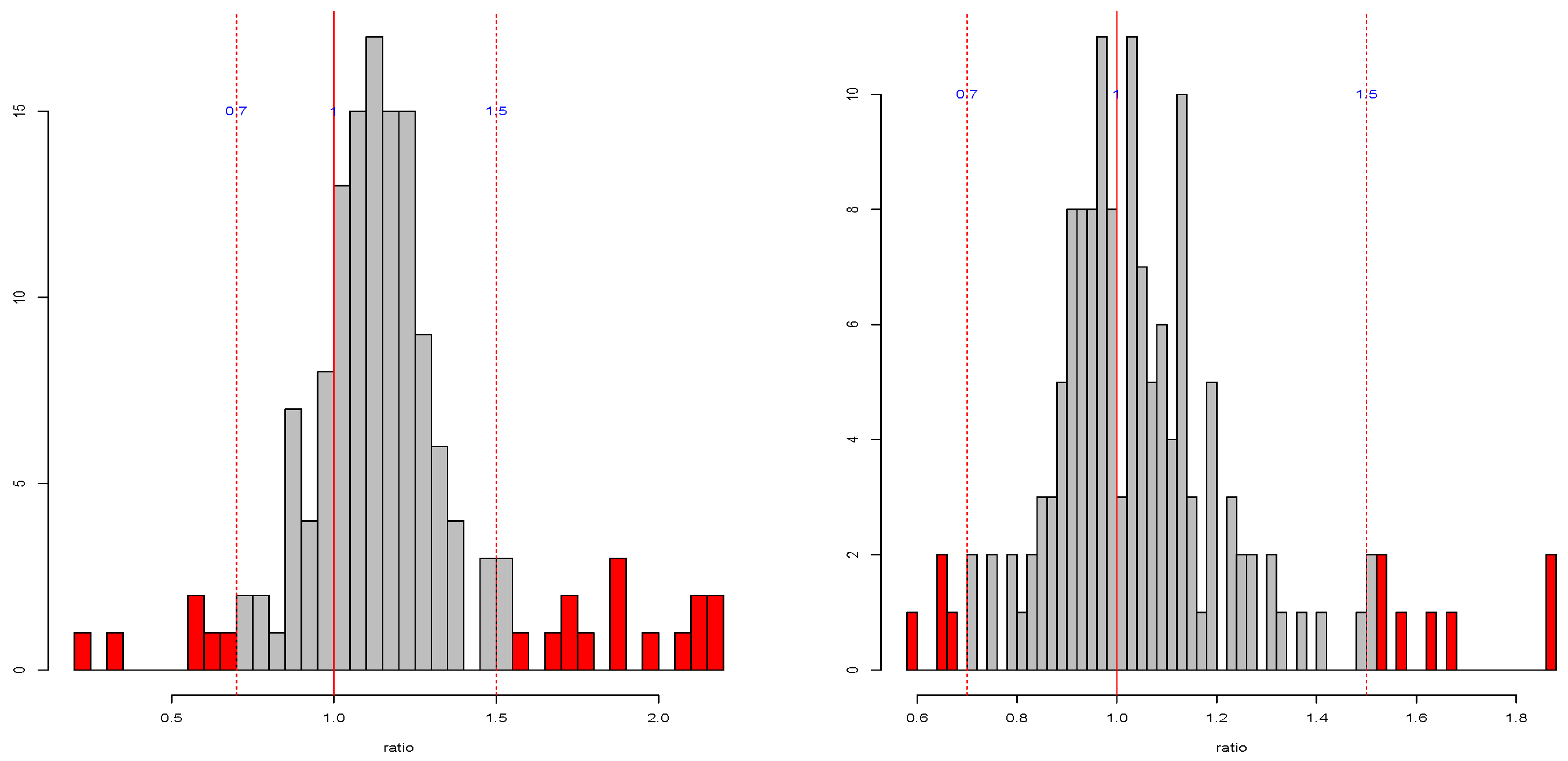
Performance assessment. Calculate the ratio of (the claimed) standard error over (the simulated true) standard deviation:

$$\frac{SE(CV.error)}{SD(CV.error)}.$$

If the 1se works well, the ratio should be close to 1. However, the results in the Table A1, Table A2, Table A3 and Table A4 show that, in some cases, the standard deviation is even more than 100% overestimated or more than 50% underestimated. The histograms of the ratios (Figure A1 and Figure A2) also show that the standard error estimates are not close to the targets. Not surprisingly, 2-fold is particularly untrustworthy. But for the common choice of 10-fold, even for independent predictors with constant coefficient, the standard error estimate by 1se can be 40% over or under the target. In addition, there is no obvious pattern on when the 1se is performing well or not. Overall, this simulation study provides evidence that the 1se fails to provide good estimation as intended (see [18] for more discussions on the standard error issues).

4.2. Is 1se Rule Better for Regression Estimation?

Since the standard error estimation in 1se is not the end goal, the poor performance of 1se in the previous subsection does not necessary mean that the 1se rule is poor for regression estimation and variable selection. In this part, we study the performance of model ${\lambda }_{1se}$ in regression estimation and compare it with that of model ${\lambda }_{min}$. A large number of samples are drawn so that we know in which cases the 1se rule can consistently outperforms the regular CV in regression estimation.

By simulations, we compare ${\lambda }_{1se}$ and ${\lambda }_{min}$ in term of accuracy in estimating the regression function. We consider several factors: nonzero coefficients ${\beta }_{\left(1\right)}$, number of zero coefficients $p-q$, sample size n, standard deviation of the noise $\sigma$ and the dependency of the predictors.

4.2.1. Model Specification

We consider the data generation model: $y=X\beta +ϵ$, where $ϵ\sim N(0,{\sigma }^2)$ and $\beta =({\beta }_{\left(1\right)},{\beta }_{\left(2\right)}),$ with ${\beta }_{\left(1\right)}=({\beta }_1,{\beta }_2$$,\dots ,{\beta }_q)$ being the nonzero coefficients and ${\beta }_{\left(2\right)}=({\beta }_{q+1},{\beta }_{q+2}$$,\dots ,{\beta }_p)$ being the zero coefficients. The vector of explanatory variables is generated by the multivariate normal distribution,

$$X\sim MV(0,{\mathsf{\Sigma }}_i),$$

where $i=1,2$.

4.2.2. Procedure

• Simulate a fixed validation set of 500 observations of the predictors for estimation of the loss.
• Each time randomly simulate a training set of n observations from the same data generating process.
• Apply the 1se rule (10-fold cross validation) over the training set and record the selected model: model with ${\lambda }_{1se}$ and the model with ${\lambda }_{min}$. Calculate the estimation losses of these two models: $\frac{1}{500}{\sum }_{i=1}^{500}{(z_i^{\prime }\widehat{\beta }-z_i^{\prime }{\beta }^{★})}^2$, where $\widehat{\beta }$ is based on ${\lambda }_{1se}$ or ${\lambda }_{min}$ respectively, and $z_i$ are independently generated from the same distribution used to generate X.
• Repeat this process for M times ($M=500$) and calculate the fraction that model with ${\lambda }_{min}$ has a smaller loss.

In our simulations, we make various comparisons: small or large nonzero coefficients; small or large error variance; small or large sample size; low- or high-dimensional data; independent or dependent design matrix. The parameter values used in our study are displayed in

Table 1. Simulation settings for regression estimation and variable selection.

Parameter	Values
${\beta }_{\left(1\right)}$	$\{0.1,1,3\}$ for constant coefficients
	$\frac{1}{i}$ where $i=1,\dots ,q$ for decaying coefficients
${\sigma }^2$	$\{0.01,4\}$
$\rho$	$\{0,0.5,0.9\}$
n	$\{100,1,000\}$
$p-q$	$\{20,990\}$ where $q=10$
${\mathsf{\Sigma }}_i$	$i=1$ for AR(1) covariance; $i=2$
	for compound symmetry covariance

below. The results are reported in

Table A5. Regression estimation: probability of ${\lambda }_{min}$ doing better, AR(1) correlation.

			Low-Dimension				High-Dimension
			$\mathit{\beta }=\mathbf{0.1}$	$\mathit{\beta }=\mathbf{1}$	$\mathit{\beta }=\mathbf{3}$	Decay $\mathit{\beta }$	$\mathit{\beta }=\mathbf{0.1}$	$\mathit{\beta }=\mathbf{1}$	$\mathit{\beta }=\mathbf{3}$	Decay $\mathit{\beta }$
$n=100$	$\rho =0$	${\sigma }^2=0.01$	0.52	0.62	1.00	0.52	0.46	0.64	0.84	0.54
		${\sigma }^2=4$	0.42	0.52	0.52	0.54	0.58	0.50	0.50	0.52
	$\rho =0.5$	${\sigma }^2=0.01$	0.54	0.83	0.92	0.52	0.58	0.70	0.90	0.58
		${\sigma }^2=4$	0.44	0.56	0.54	0.58	0.38	0.60	0.60	0.60
	$\rho =0.9$	${\sigma }^2=0.01$	0.56	0.88	1.00	0.60	0.54	0.84	0.96	0.54
		${\sigma }^2=4$	0.54	0.56	0.56	0.54	0.57	0.52	0.52	0.46
$n=1000$	$\rho =0$	${\sigma }^2=0.01$	0.58	0.57	NaN	0.58	0.64	0.71	NaN	0.74
		${\sigma }^2=4$	0.45	0.58	0.56	0.52	0.57	0.66	0.66	0.72
	$\rho =0.5$	${\sigma }^2=0.01$	0.50	NaN	NaN	0.54	0.68	NaN	NaN	0.68
		${\sigma }^2=4$	0.52	0.50	0.52	0.54	0.64	0.68	0.68	0.70
	$\rho =0.9$	${\sigma }^2=0.01$	0.56	NaN	NaN	0.60	0.66	NaN	NaN	0.70
		${\sigma }^2=4$	0.56	0.54	0.58	0.54	0.68	0.66	0.64	0.66

and

Table A6. Regression estimation: probability of ${\lambda }_{min}$ doing better, constant correlation.

			Low-Dimension				High-Dimension
			$\mathit{\beta }=\mathbf{0.1}$	$\mathit{\beta }=\mathbf{1}$	$\mathit{\beta }=\mathbf{3}$	Decay $\mathit{\beta }$	$\mathit{\beta }=\mathbf{0.1}$	$\mathit{\beta }=\mathbf{1}$	$\mathit{\beta }=\mathbf{3}$	Decay $\mathit{\beta }$
$n=100$	$\rho =0.5$	${\sigma }^2=0.01$	0.56	0.88	0.89	0.53	0.54	0.84	1.00	0.64
		${\sigma }^2=4$	0.53	0.56	0.54	0.52	0.61	0.52	0.56	0.60
	$\rho =0.9$	${\sigma }^2=0.01$	0.60	1.00	1.00	0.70	0.56	0.82	0.90	0.70
		${\sigma }^2=4$	0.58	0.54	0.62	0.62	0.62	0.58	0.64	0.64
$n=1000$	$\rho =0.5$	${\sigma }^2=0.01$	0.50	NaN	NaN	0.50	0.74	NaN	NaN	0.78
		${\sigma }^2=4$	0.50	0.42	0.50	0.44	0.72	0.74	0.76	0.78
	$\rho =0.9$	${\sigma }^2=0.01$	0.48	NaN	NaN	0.54	0.74	NaN	NaN	0.78
		${\sigma }^2=4$	0.52	0.50	0.52	0.46	0.72	0.74	0.76	0.76

. Note that when ${\lambda }_{min}$ and ${\lambda }_{1se}$ give identical selection over the $M=500$ runs, the entry in the table is NaN.

The simulation results show that, in general, for the design matrix with either AR(1) correlation or constant correlation, the model with ${\lambda }_{min}$ tends to provide better regression estimation (with smaller estimation errors), especially when the data is generated with relatively large coefficient. In addition, we consider two more settings below.

4.2.3. Case 1: Large $p/q$

In this case, we consider high-dimensional data with AR(1) covariance design matrix, ${\mathsf{\Sigma }}_1$, where $q=10$ and $p=1000$. We set ${\sigma }^2=1$, $n\in \{100,1000\}$, $\rho \in \{0.01,0.9\}$, constant nonzero coefficients with value $\beta \in \{1,6,11,16,21\}$. We report the probability that model ${\lambda }_{min}$ estimates better. Clearly, in this case, the model ${\lambda }_{min}$ significantly outperforms the model ${\lambda }_{1se}$ for a range of $\beta$ values at both sample size (See Figure 1).

4.2.4. Case 2: Small $p/q$

In this case, we consider low-dimensional data with AR(1) covariance design matrix, ${\mathsf{\Sigma }}_1$, where $q=10$ and $p-q\in \{2,5,10\}$. We set ${\sigma }^2=0.01$, $n\in \{100,1000\}$, $\rho =0.1$, the common nonzero coefficient value $\beta \in \{0.2,0.4,0.6,0.8,1,$$1.2\}$. We report the probability that model ${\lambda }_{min}$ estimates the regression function better. In this case, model ${\lambda }_{min}$ significantly outperforms model ${\lambda }_{1se}$ as the common coefficient value increases over 1, getting close to or even over 0.8 (See Figure 2).

4.3. Is 1se Rule Better for Variable Selection?

There are two main issues of the application of the 1se rule in variable selection. One is that the accuracy of variable selection by Lasso itself is very sensitive to the parameter values in the data generating process. In various situations (especially when the covariance are complicatedly correlated such as in gene expression type of data), Lasso may perform very poorly in accurate variable selection. The second issue is that ${\lambda }_{min}$ and ${\lambda }_{1se}$ returned by the glmnet function are the same in many cases and then there is no difference in the result of variable selection. The cases where ${\lambda }_{min}={\lambda }_{1se}$ are eliminated in the following general study. To examine the real difference between ${\lambda }_{min}$ and ${\lambda }_{1se}$, we consider the difference of their probabilities of selecting the true model given that they have distinct select outcome.

4.3.1. Procedure

• Randomly simulate a data set of sample size n given the parameter values.
• Perform variable selection with ${\lambda }_{min}$ and ${\lambda }_{1se}$ over the simulated data set, respectively. If the two returned models are the same, then discard the result and go back to step 1. Otherwise, check their variable selection results.
• Repeat the above process for M times ($M=500$) and calculate the fraction of correct variable selection, denoted by $P_c\left({\lambda }_{1se}\right)$ and $P_c\left({\lambda }_{min}\right)$, respectively. We report the proportion difference $P_c\left({\lambda }_{1se}\right)-P_c\left({\lambda }_{min}\right)$. Positive means 1se rule is better.

We adopt the same framework and parameter settings (Table 1) as that used for regression estimation. The results show that ${\lambda }_{1se}$ tends to outperform ${\lambda }_{min}$ in most of the cases when the data are generated with AR(1) correlation design matrix (see

Table A7. Variable selection: $P_c\left({\lambda }_{1se}\right)-P_c\left({\lambda }_{min}\right)$, AR(1) correlation.

			Low-Dimension				High-Dimension
			$\mathit{\beta }=\mathbf{0.1}$	$\mathit{\beta }=\mathbf{1}$	$\mathit{\beta }=\mathbf{3}$	Decay $\mathit{\beta }$	$\mathit{\beta }=\mathbf{0.1}$	$\mathit{\beta }=\mathbf{1}$	$\mathit{\beta }=\mathbf{3}$	Decay $\mathit{\beta }$
$n=100$	$\rho =0$	${\sigma }^2=0.01$	0.13	0.13	0	0.06	0	0	0.02	NaN
		${\sigma }^2=4$	0	0.12	0.11	0.01	0	0	0	0.90
	$\rho =0.5$	${\sigma }^2=0.01$	0.45	0	0	0	0.25	0.01	0	NaN
		${\sigma }^2=4$	0	0.40	0.43	0.05	0	0.16	0.27	0.87
	$\rho =0.9$	${\sigma }^2=0.01$	0.40	0	0	0	0.61	0	0	NaN
		${\sigma }^2=4$	0	0.14	0.39	0.01	0	0.25	0.62	0.7
$n=1000$	$\rho =0$	${\sigma }^2=0.01$	0.72	0.10	NaN	0.70	0.27	0.16	NaN	NaN
		${\sigma }^2=4$	0	0.71	0.70	0	0	0.25	0.25	0.52
	$\rho =0.5$	${\sigma }^2=0.01$	0.86	NaN	NaN	0.03	0.86	NaN	NaN	NaN
		${\sigma }^2=4$	0	0.85	0.85	0	0	0.85	0.85	0.95
	$\rho =0.9$	${\sigma }^2=0.01$	0.56	NaN	NaN	0	0.76	NaN	NaN	NaN
		${\sigma }^2=4$	0	0.67	0.36	0	0	0.77	0.17	0.65

and

Table A8. Variable selection: $P_c\left({\lambda }_{1se}\right)-P_c\left({\lambda }_{min}\right)$: constant correlation.

			Low-Dimension				High-Dimension
			$\mathit{\beta }=\mathbf{0.1}$	$\mathit{\beta }=\mathbf{1}$	$\mathit{\beta }=3$	Decay $\mathit{\beta }$	$\mathit{\beta }=\mathbf{0.1}$	$\mathit{\beta }=\mathbf{1}$	$\mathit{\beta }=\mathbf{3}$	Decay $\mathit{\beta }$
$n=100$	$\rho =0.5$	${\sigma }^2=0.01$	0	0	0.1	0	0	0	0	0
		${\sigma }^2=4$	0	0	0	0	0	0	0	0
	$\rho =0.9$	${\sigma }^2=0.01$	0	0	0	0	0	0	0	0
		${\sigma }^2=4$	0	0	0	0	0	0	0	0
$n=1000$	$\rho =0.5$	${\sigma }^2=0.01$	0	NaN	NaN	0.01	0	NaN	NaN	0
		${\sigma }^2=4$	0	0	0	0	0	0	0	0
	$\rho =0.9$	${\sigma }^2=0.01$	0	NaN	NaN	0.01	0	NaN	NaN	0
		${\sigma }^2=4$	0	0	0	0	0	0	0	0

). But with constant correlation design matrix, these two methods have no practically difference in variable selection.

Below we consider several special cases where model ${\lambda }_{min}$ still needs to be considered, and although it can only do slightly better when the error variance is large, nonzero coefficients are small and no extra variables exist to interrupt the selection process.

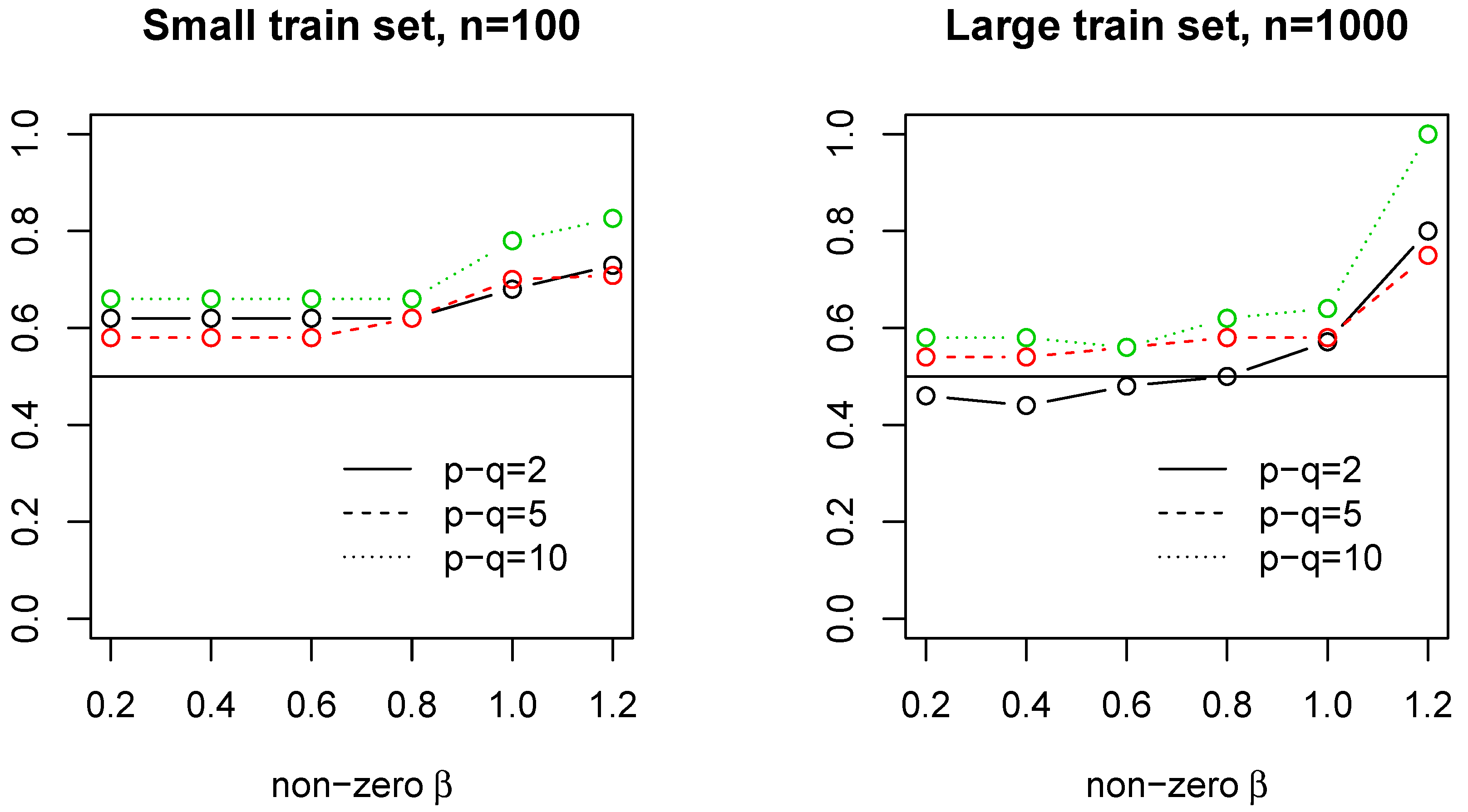
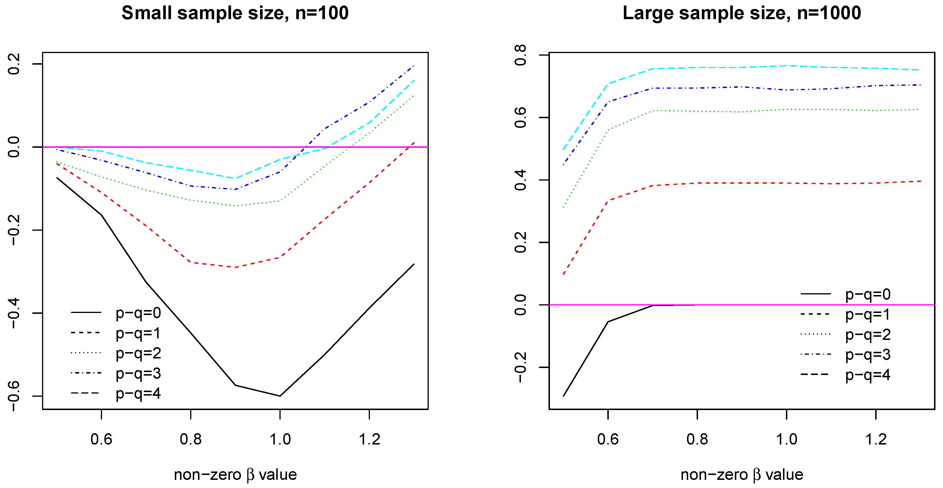
4.3.2. Case 1: Constant Coefficients

In this case, let $q=5$, $p-q\in \{0,1,2,3,4\}$, ${\sigma }^2=4$, $n\in \{100,1000\}$, $\rho =0.01$ and the common nonzero $\beta \in [0.5,1.3]$ with ${\mathsf{\Sigma }}_1$. The result is in Figure 3. In the case of small sample size, say $n=100$, model ${\lambda }_{min}$ has higher probability of correct variable selection when the constant coefficient lies between (0.5,1). The largest difference appears when $p-q=0$, not surprisingly. As the common coefficient value becomes larger than 1, the probability increases from negative to positive, which indicates the reverse to be true: model ${\lambda }_{1se}$ now works better. However, in the case of large sample size, say $n=1000$, model ${\lambda }_{1se}$ significantly outperforms model ${\lambda }_{min}$ unless when $p-q=0$.

4.3.3. Case 2: Decaying Coefficients

In this case, let $q=5$, ${\sigma }^2=4$, $n=1000$, $\rho =0.5$, $p-q\in 0,5,10,15,20,25,30,35,40,45,50$, and ${\beta }_i=\frac{1}{i}$, $i=1,2,\dots ,q$ with ${\mathsf{\Sigma }}_1$. Figure 4 indicates that, with decaying coefficients lie between (0,1) and large sample size $n=1000$, model ${\lambda }_{min}$ has higher probability of correct variable selection when the number of zero-coefficient variables $p-q$ is small. The largest difference appears when $p-q=0$, i.e., there is no extra variables provided to interrupt the variable selection process.

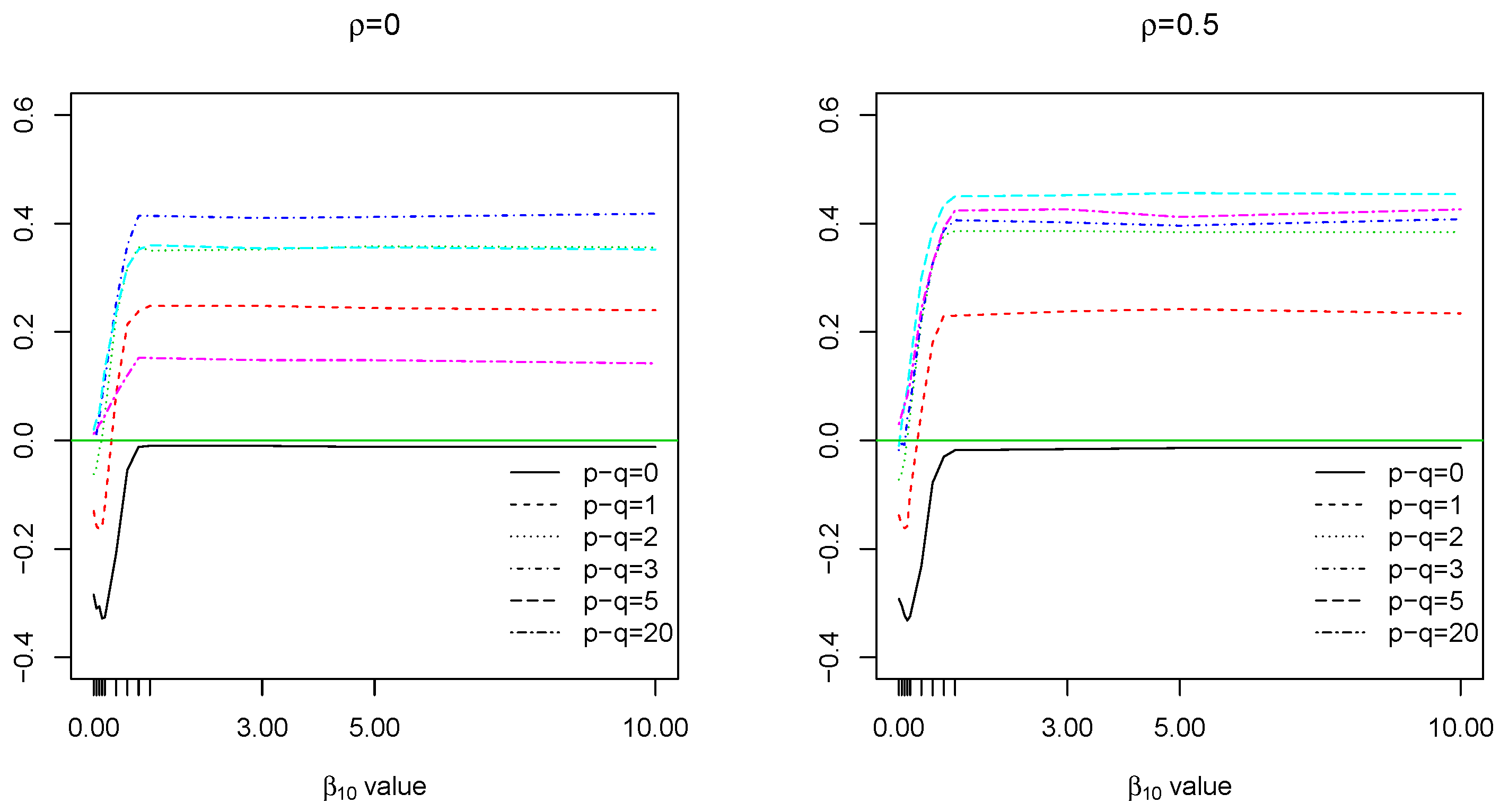
4.3.4. Case 3: Hybrid Case

Let $n=100$, ${\sigma }^2=4$ and $\rho \in \{0,0.5\}$ with ${\mathsf{\Sigma }}_1$. In this data generating process, we set the first ten coefficients to be positive, i.e., $q=10$, among which the first nine nonzero coefficients are constant 1, while the last one ${\beta }_{10}$ increases from 0 to 10, i.e., ${\beta }_{10}\in \{0,0.05,0.1,0.15,0.2,0.4,0.6,0.8,1,3,5,10\}$. The number of zero coefficients $p-q\in \{0,1,2,3,$$5,20\}$. From Figure 5, when ${\beta }_{10}$ is very small, i.e., ${\beta }_{10}\in \{0.05,0.2\}$ and $p-q=0$, ${\lambda }_{min}$ performs better. For other situations, ${\lambda }_{1se}$ is significantly better.

5. Data Examples

In this section, the performances of the 1se rule and the regular CV in regression estimation and variable selection are examined over real data sets: Boston Housing Price (an example of $n>p$) and Bardet–Biedl data (an example of $p>n$).

Boston Housing Price. The data were collected by [19] for the purpose of discovering whether or not clean air influenced the value of houses in Boston. It consists of 506 observations and 14 non constant independent variables. Of these, medv is the response variable while the other 13 variables are possible predictors.

Bardet–Biedl. The gene expression data are from the microarray experiments of mammalianeye tissue samples of [20]. The data consists of 120 rats with 200 gene probes and the expression level of TRIM32 gene. It is interesting to know which gene probes are more able to explain the expression level of TRIM32 gene by regression analysis.

5.1. Regression Estimation

To test which method does better in regression estimation, we perform both cross validation and data guided simulation (DGS) over these two real data sets as follows.

5.1.1. Procedure for Cross Validation

• We randomly select $n_1$ observations from the data sets as training set and the rest as validation set, $n_1\in \{100,200,$$400\}$ for Boston Housing Price and $n_1\in \{40,80\}$ for Bardet–Biedl data.
• Apply K-fold cross validation $K\in \{5,10,20\}$, for Boston Housing Price and $K\in \{5,10\}$ for Bardet–Biedl data over the training set and compute the mean square prediction error of model ${\lambda }_{1se}$ and model ${\lambda }_{min}$ over the validation set.
• Repeat the above process for 500 times and compute the proportion of better estimation for each method.

The results (

Table 2. Regression estimation (cross validation): Boston Housing Price.

Proportion of ${\mathit{\lambda }}_{\mathbf{min}}$ Being Better in Prediction
	5-fold	10-fold	20-fold
train set $n_1=100$	0.554	0.526	0.538
train set $n_1=200$	0.560	0.556	0.564
train set $n_1=400$	0.552	0.564	0.558

and

Table 3. Regression estimation (cross validation): Bardet–Biedl.

Proportion of ${\mathit{\lambda }}_{\mathbf{min}}$ Being Better in Prediction
	5-fold	10-fold
train set $n_1=40$	0.582	0.566
train set $n_1=80$	0.580	0.594

) show that, for all the training size $n_1$ considered, the proportion of model ${\lambda }_{min}$ doing better is about 52∼57% for Boston Housing Price; 56∼59% for Bardet–Biedl data. The consistent slight advantage of ${\lambda }_{min}$ agrees with our earlier simulation results in supporting ${\lambda }_{min}$ as the better method for regression estimation.

5.1.2. Procedure for DGS

• Obtain model ${\lambda }_{min}$ and model ${\lambda }_{1se}$ with K-fold cross validation, $K\in \{5,10,20\}$, over the data and also the coefficient estimates ${\widehat{\beta }}_{min}$, ${\widehat{\beta }}_{1se}$, the standard deviation estimates ${\widehat{\sigma }}_{min}$, ${\widehat{\sigma }}_{1se}$ and the estimated responses ${\widehat{y}}_{min,1}$, ${\widehat{y}}_{1se,1}$ (fitted values).
• Simulate the new responses in two scenarios:
  Scenario 1: $y={\widehat{y}}_{min,1}+ϵ$ with $ϵ\sim N(0,{\widehat{\sigma }}_{min}^{2}I)$,
  Scenario 2: $y={\widehat{y}}_{1se,1}+ϵ$ with $ϵ\sim N(0,{\widehat{\sigma }}_{1se}^{2}I)$.
• Here, apply Lasso with ${\lambda }_{min}$ and ${\lambda }_{1se}$ (using the same K-fold CV) on the new data set (i.e., new response and the original design matrix) and get the new estimated responses ${\widehat{y}}_{min,2}$ and ${\widehat{y}}_{1se,2}$ for each of the two scenarios.
• Calculate the mean square estimation error $\frac{1}{n}{\sum }_{i=1}^n{({\widehat{y}}_{min,2}-{\widehat{y}}_{min,1})}^2$ and $\frac{1}{n}{\sum }_{i=1}^n{({\widehat{y}}_{1se,2}-{\widehat{y}}_{min,1})}^2$ for scenario 1;
  $\frac{1}{n}{\sum }_{i=1}^n{({\widehat{y}}_{min,2}-{\widehat{y}}_{1se,1})}^2$ and $\frac{1}{n}{\sum }_{i=1}^n{({\widehat{y}}_{1se,2}-{\widehat{y}}_{1se,1})}^2$ for scenario 2.
• Repeat the above resampling process for 500 times and compute the proportion of better estimation for each method.

The estimation results (

Table 4. Regression estimation (DGS).

Proportion of ${\mathit{\lambda }}_{\mathbf{min}}$ Being Better in Estimation
	Boston Housing Price			Bardet–Biedl
	5-fold	10-fold	20-fold	5-fold	10-fold
Scenario 1	0.478	0.486	0.468	0.528	0.523
Scenario 2	0.515	0.489	0.487	0.494	0.480

) show that, overall, the proportion of better estimation for the model ${\lambda }_{min}$ is between 46.8∼52.8% and for the model ${\lambda }_{1se}$, it is between 47.2∼53.2%. Therefore, based on the DGS, in term of regression estimation accuracy, there is not much difference before ${\lambda }_{min}$ and ${\lambda }_{1se}$: the observed properties are not significantly different from 50% at 0.05 level.

5.2. Variable Selection: DGS

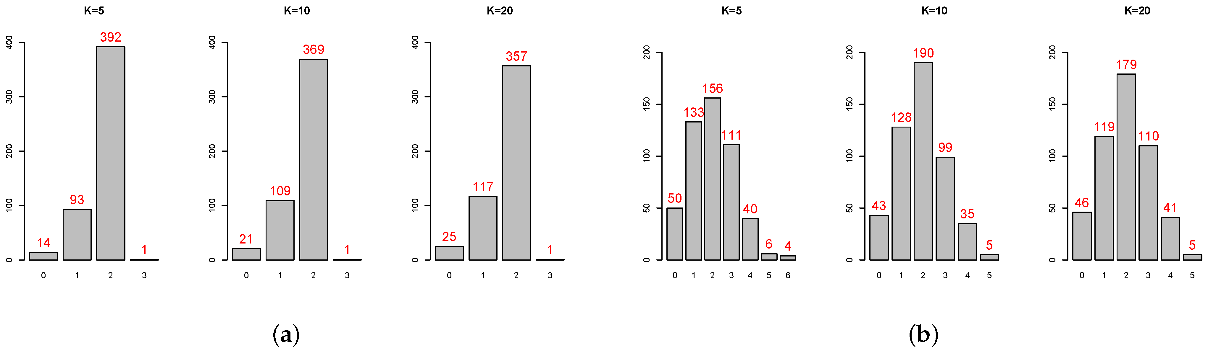
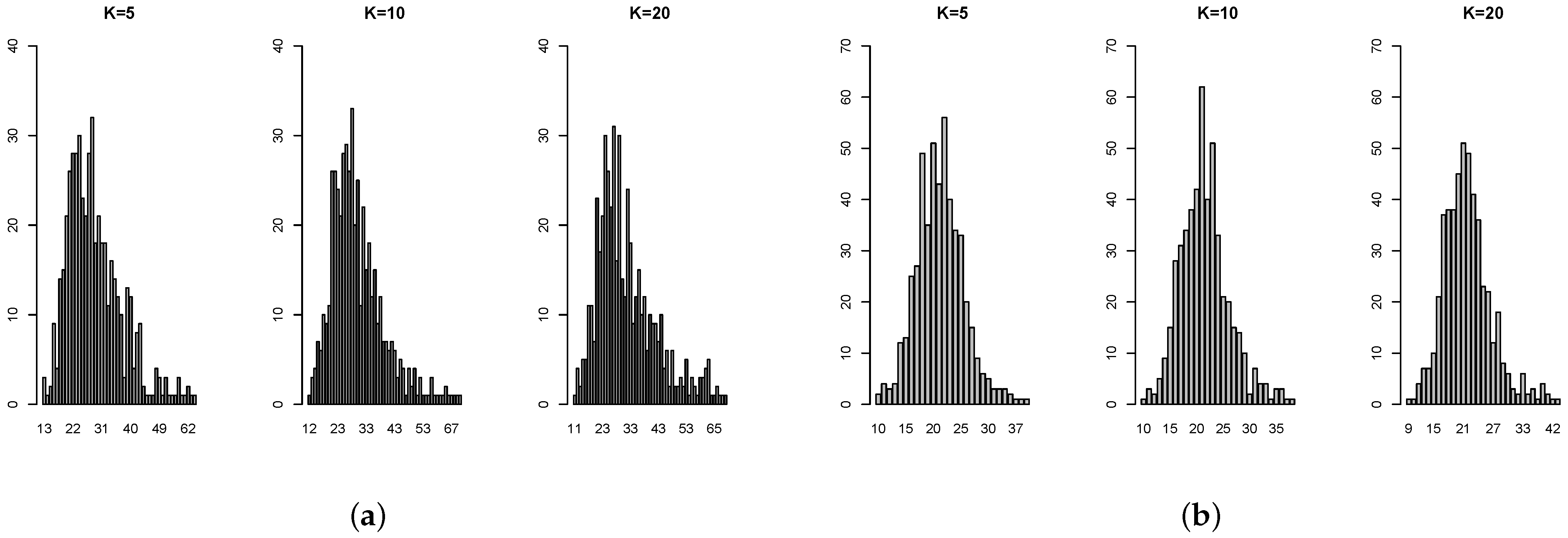
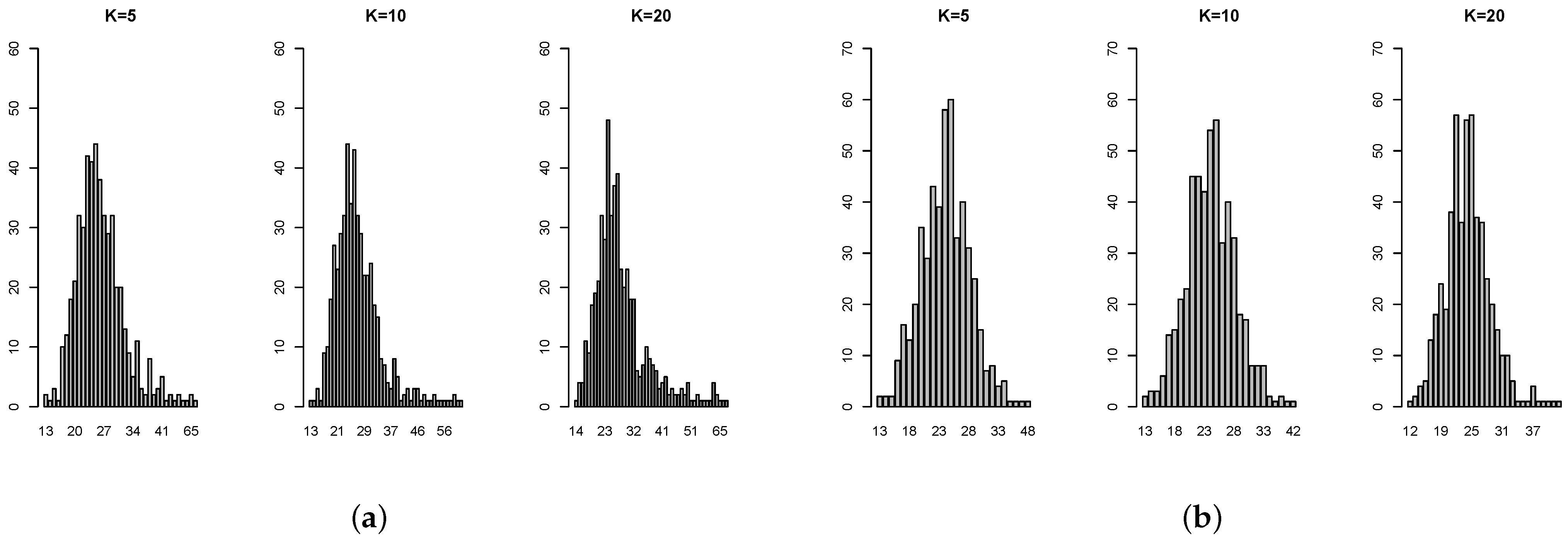
To test which model does better in variable selection, we perform the DGS over the above real data sets. Since the exact variable selection might not be reached, especially when applied to the high-dimensional data, we use symmetric difference $\mid S^{★}▽\widehat{S}\mid$ to measure their performance, which is the number of variables either in $S^{★}$ but not in $\widehat{S}$ or in $\widehat{S}$ but not in $S^{★}$. Below is the algorithm for the DGS.

Procedure

• Apply the 10-fold (default) cross validation over real data set and select the true set of variables $S^{★}$: $S_{min}^{★}$ or $S_{1se}^{★}$, either by the model with ${\lambda }_{min}$ or by the model with ${\lambda }_{1se}$.
• Do least square estimation by regressing the response on the true set of variables and obtain the estimated response $\widehat{y}$ and the residual standard error $\widehat{\sigma }$.
• Simulate the new response $y_{new}$ by adding the error term randomly generated from $N(0,{\widehat{\sigma }}^2)$ to $\widehat{y}$. Apply K-fold cross validation, $K\in \{5,10,20\}$, over the simulated data set (i.e., $y_{new}$ and the original design matrix) and select set of variables $\widehat{S}$: ${\widehat{S}}_{min}$ or ${\widehat{S}}_{1se}$, either by model ${\lambda }_{min}$ or by model ${\lambda }_{1se}$. Repeat this process for 500 times.
• Calculate the symmetric difference $\mid S^{★}▽\widehat{S}\mid$.

The distributions of the symmetric difference are shown in the appendix. (Figure A3 and Figure A4 for Boston Housing Price; Figure A5 and Figure A6 for Bardet–Biedl data) The mean of $\mid \widehat{S}\mid$ is reported in

Table 5. Mean of selected model size $\mid \widehat{S}\mid$: Boston Housing Price.

		5-fold	10-fold	20-fold
$\mid S_{min}^{★}\mid =11$	$\mid {\widehat{S}}_{min}\mid$	12.744	12.672	12.636
	$\mid {\widehat{S}}_{1se}\mid$	10.564	10.608	10.560
$\mid S_{1se}^{★}\mid =8$	$\mid {\widehat{S}}_{min}\mid$	10.792	10.824	10.772
	$\mid {\widehat{S}}_{1se}\mid$	8.250	8.254	8.246

and

Table 6. Mean of selected model size $\mid \widehat{S}\mid$: Bardet–Biedl.

		5-fold	10-fold	20-fold
$\mid S_{min}^{★}\mid =21$	$\mid {\widehat{S}}_{min}\mid$	32.272	33.604	35.500
	$\mid {\widehat{S}}_{1se}\mid$	21.064	21.864	22.404
$\mid S_{1se}^{★}\mid =19$	$\mid {\widehat{S}}_{min}\mid$	24.208	25.426	26.350
	$\mid {\widehat{S}}_{1se}\mid$	19.852	19.992	20.274

. For Boston Housing Price, the size of the candidate variables is 13 while model ${\lambda }_{min}$ selects 11 variables and model ${\lambda }_{1se}$ selects 8 variables on average, i.e., the mean of $\mid S_{min}^{★}\mid$ is 11 and the mean of $\mid S_{1se}^{★}\mid$ is 8. For Bardet–Biedl data, the size of the candidate variables is 200, while model ${\lambda }_{min}$ selects 21 variables and model ${\lambda }_{1se}$ selects 19 variables on average, i.e., the mean of $\mid S_{min}^{★}\mid$ is 21 and the mean of $\mid S_{1se}^{★}\mid$ is 19.

On average, the 1se rule does better in variable selection since the mean of $\mid {\widehat{S}}_{1se}\mid$ is more closed to $\mid S^{★}\mid$. In the case of $n>p$, if we want to have a perfect or near perfect variable selection result (i.e., $\mid S^{★}▽\widehat{S}\mid \le 1$), then the 1se rule is a good choice, despite the fact that its selection result is more unstable: the range of $\mid S^{★}▽{\widehat{S}}_{1se}\mid$ is larger than that of $\mid S^{★}▽{\widehat{S}}_{min}\mid$. In the case of $n<p$, both models fail to provide perfect selection result. But overall the 1se rule is more accurate and stable given that $\mid S^{★}▽{\widehat{S}}_{1se}\mid$ has smaller mean and range.

6. Conclusions

The one standard error rule is proposed to pick the most parsimonious model within one standard error of the minimum. Despite the fact that it was widely used as a conservative and alternative approach for cross validation, there is no evidence confirming that the 1se rule can consistently outperform the regular CV.

Our theoretical result shows that the standard error formula is asymptotically valid when the regression procedure converges relatively fast to the true regression function. Our illustrative example also shows that when the regression estimator converges slowly, the CV errors on the different evaluation folds may be highly dependent, which unfortunately makes the usual sample variance (or sample standard deviation) formula problematic. In such a case, the use of the 1se rule may easily lead to a choice of inferior candidates.

Our numerical results offer finite-sample understandings. First of all, the simulation study also casts doubt on the estimation accuracy of the 1se rule in terms of estimating the standard error of the minimum cross validation error. In some cases, the 1se is likely to have 100% overestimation or underestimation, depending on the number of cross validation fold and the dependency among the predictors. More specifically, for example, the 1se tends to have overestimation when used with 2-fold cross validation in case of dependent predictors; but it tends to have underestimation when used with 20-fold cross validation in case of independent predictors.

Secondly, the performances of the 1se rule and the regular CV in regression estimation and variable selection are compared via both simulated and real data sets. In general, on the one hand, the 1se rule often performs better in variable selection for sparse modeling; on the other hand, it often does worse in regression estimation.

While our theoretical and numerical results clearly challenge indiscriminate uses of the 1se rule in general model selection, its parsimony nature may still be appealing when a sparse model is highly desirable. For the real data sets, for regression estimation, the regular CV does better than the 1se rule but the difference is small. There is almost no difference in the estimation accuracy between these two methods when regression estimation is assessed by the DGS. Overall, considering the model simplicity and interpretability, the 1se rule would be a better choice here.

Future studies are encouraged to provide more theoretical understandings on the 1se rule. Also, it may be studied numerically in more complex settings (e.g., when used to compare several nonlinear/nonparametric classification methods) than those in this work. In a larger context, since it is well known that the penalty methods for model selection are often unstable (e.g., [1,21,22]), alternative methods to strengthen reliability and reproductivity of variable selection may be applied (see reference in the above mentioned papers and [23]).