Article

Unsupervised Feature Selection for Histogram-Valued Symbolic Data Using Hierarchical Conceptual Clustering

1
School of Science and Engineering, Tokyo Denki University, Hatoyama, Saitama 350-0394, Japan
2
Department of Computer Systems, Tallinn University of Technology, Ehitajate tee 5, 19086 Tallinn, Estonia
*
Author to whom correspondence should be addressed.
Stats 2021, 4(2), 359-384; https://doi.org/10.3390/stats4020024
Submission received: 30 March 2021 / Revised: 22 April 2021 / Accepted: 12 May 2021 / Published: 18 May 2021
(This article belongs to the Special Issue Recent Developments in Clustering and Classification Methods)

Abstract

:
This paper presents an unsupervised feature selection method for multi-dimensional histogram-valued data. We define a multi-role measure, called the compactness, based on the concept size of given objects and/or clusters described using a fixed number of equal probability bin-rectangles. In each step of clustering, we agglomerate objects and/or clusters so as to minimize the compactness for the generated cluster. This means that the compactness plays the role of a similarity measure between objects and/or clusters to be merged. Minimizing the compactness is equivalent to maximizing the dis-similarity of the generated cluster, i.e., concept, against the whole concept in each step. In this sense, the compactness plays the role of cluster quality. We also show that the average compactness of each feature with respect to objects and/or clusters in several clustering steps is useful as a feature effectiveness criterion. Features having small average compactness are mutually covariate and are able to detect a geometrically thin structure embedded in the given multi-dimensional histogram-valued data. We obtain thorough understandings of the given data via visualization using dendrograms and scatter diagrams with respect to the selected informative features. We illustrate the effectiveness of the proposed method by using an artificial data set and real histogram-valued data sets.

1. Introduction

Unsupervised feature selection is important in pattern recognition, data mining, and generally in data science (e.g., [1,2,3,4]). Solorio-Fernández et al. [4] evaluated and discussed many filter, wrapper, and hybrid methods, and they showed a detail classification of unsupervised feature selection methods. They also pointed out the challenge for complex data models is one of the important themes in unsupervised feature selection. Bock and Diday [5] and Billard and Diday [6] include methods of Symbolic Data Analysis (SDA) for complex data models. Diday [7] presents an overview of SDA in data science, and Billard and Diday [8] present various methods to analyze symbolic data including histogram-valued data.
In unsupervised feature selection, we need a mechanism to detect meaningful structures organized by the data set under the given feature set. Geometrically thin structures such as functional structures and multi-cluster structures are examples of meaningful structures of the data set. Many unsupervised feature selection methods use clustering to search feature subspaces including meaningful structures. Therefore, we have to solve the following four problems:
(1)
How to evaluate the similarity between objects and/or clusters under the given feature subset;
(2)
How to evaluate the quality of clusters under the given feature subset;
(3)
How to evaluate the effectiveness of the given feature subset; and
(4)
How to search the most robustly informative feature subset from the whole feature set.
In hierarchical agglomerative methods, as noted in Billard and Diday [8], we select a (dis)similarity measure between objects and we obtain a dendrogram by merging objects and/or clusters based on the selected criterion, e.g., nearest neighbor, furthest neighbor, Ward’s minimum variance, or other criteria. For histogram-valued data, Irpino and Verde [9] defined the Wasserstein distance and proposed a hierarchical clustering method based on Ward’s criterion. As a non-hierarchical clustering method, De Carvarho and De Souza [10] proposed the dynamical clustering method optimizing an adequacy criterion. By combining these methods with an appropriate wrapper method, for example, we can realize unsupervised feature selection methods for histogram-valued data.
This paper presents an unsupervised feature selection method for mixed-type histogram-valued data by using hierarchical conceptual clustering based on the compactness. The compactness defines the concept size of rectangles describing objects and/or clusters in the given feature space.
In the proposed method, the compactness plays not only the role of similarity measure between objects and/or clusters, but also the roles of cluster quality criterion and feature effectiveness criterion. Therefore, we can greatly simplify to realize the unsupervised feature selection method for complex, histogram-valued symbolic data.
The structure of this paper is as follows: Section 2 describes the quantile method to represent multi-dimensional distributional data. When the given p distributional features describe each of N objects, we use histogram representations for various feature types including categorical multi-value and modal multi-value types. We transform each feature value of each object to the predetermined common number m of bins and their bin probabilities. We define m + 1 quantile vectors ordered from the minimum quantile vector to the maximum quantile vector in order to describe each object in the p dimensional histogram-valued feature space. We define m series of p dimensional bin-rectangles spanned by the successive quantile vectors to have common descriptions for the given objects. Then, we define the concept size of each of m bin-rectangles using the arithmetic average of p normalized bin-widths, respectively. Section 3 describes the measure of compactness for the merged objects and/or clusters. For an arbitrary pair of objects and for each histogram-valued feature, we define the average cumulative distribution function based on the two histogram values, and we find m + 1 quantile values including the minimum and the maximum values from the obtained cumulative distribution function for each of p features. Then, we obtain m series of p-dimensional bin rectangles with predetermined bin probabilities in order to define the Cartesian join of the pair of objects in the p-dimensional feature space. Under the assumption of equal bin probabilities, we define a new similarity measure, the compactness, of a pair of objects and/or clusters as the average of m concept sizes of bin-rectangles obtained for the pair. Section 4 describes the proposed method of hierarchical conceptual clustering (HCC) and exploratory method of feature selection, and then we show the effectiveness of the proposed method using artificial data and using four real data sets, including comparisons with the results by Irpino and Verde [9] and De Carvalho and De Souza [10]. Section 5 is a discussion of the obtained results.

2. Representation of Objects by Bin-Rectangles

Let U = {ωi, i = 1, 2,…, N} be the set of given objects, and let features Fj, j = 1, 2,…, p, describe each object. Let Dj be the domain of feature Fj, j =1, 2, …, p. Then, the feature space is defined by
D(p) = D1 × D2 ×⋅⋅⋅× Dp
Since we permit the simultaneous use of various feature types, we use the notation D(p) for the feature space in order to distinguish it from usual p-dimensional Euclidean space Rp. Each element of D(p)is represented by
E = E1 × E2 ×⋅⋅⋅× Ep,
where Ej, j = 1, 2, , p, is the feature value taken by the feature Fj.

2.1. Histogram-Valued Feature

For each object ωi, let each feature Fj be represented by histogram value:
Eij = {[aijk, aij(k+1)), pijk; k = 1, 2,…, nij},
where pij1 + pij2 + … + pijnij = 1 and nij is the number of bins that compose the histogram Eij.
Therefore, the Cartesian product of p histogram values represents an object ωi:
Ei = Ei1 × Ei2 ×⋯× Eip.
Since the interval-valued feature is a special case of histogram feature with nij = 1 and pij1 = 1, the representation of (3) is reduced to an interval:
Eij = [aij1, aij2).

2.2. Histogram Representation of Other Feature Types

2.2.1. Categorical Multi-Valued Feature

Let Fj be a categorical multi-valued feature, and let Eij be a value of Fj for an object ωi. The value Eij contains one or more categorical values taken from the domain Dj that is composed of finite possible categorical values. For example, Eij = {“white”, “green”} is a value taken from the domain Dj = {“white”, “red”, “blue”, “green”, “black”}. For this kind feature value, we can again use a histogram. For each value in domain Dj, we assign an interval with equal width. Then, assuming uniform probability for values in a multi-valued feature, we assign probabilities to each interval associated with a specific value in Dj according to its presence in Eij. Therefore, the feature value Eij = {“white”, “green”}, for example, is now represented by the histogram Eij = {[0, 1)0.5, [1, 2)0, [2, 3)0, [3, 4)0.5, [4, 5)0}.

2.2.2. Modal Multi-Valued Feature

Let Dj = {ν1, ν2,…, νn} be a finite list of possible outcomes and be the domain of a modal multi-valued feature Fj. A feature value Eij for object ωi is a subset of Dj with a nonnegative measure attached to each of the values in that subset, and the sum of those nonnegative measures is one:
Eij = {νij1, pij1; νij2, pij2;…; νijnij, pijnij},
where {νij1, νij2,…, νijnij}⊆Dj, νijk occurs with the nonnegative weight pijk, k = 1, 2, …, nij, and with pij1 + pij2 +… + pijnij = 1.
For example, Eij = {“white”, 0.8; “green”, 0.2} is a value of the modal multi-valued feature defined on the domain Dj = {“white”, “red”, “blue”, “green”, “black”}. We assign again a same sized interval to each possible feature value from the domain Dj. The probabilities assigned to a specific feature value of the modal multi-valued feature are used as the bin probabilities of the corresponding histogram with the same bin width. Therefore, in the above example, we have a histogram representation: Eij = {[0, 1)0.8, [1, 2)0, [2, 3)0, [3, 4)0.2, [4, 5)0}.

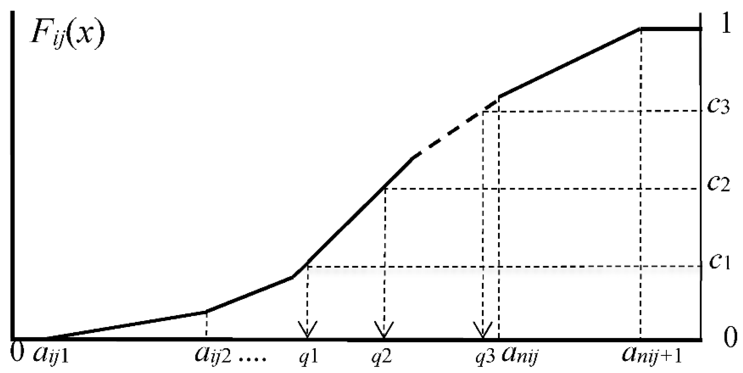
2.3. Representation of Histograms by Common Number of Quantiles

Let ωiU be the given object, and let Eij in (7) be the histogram value for a feature Fj:
Eij = {[aijk, aij(k+1)), pijk; k = 1, 2,…, nij}.
Then, under the assumption that nij bins have uniform distributions, we define the cumulative distribution function Fij(x) of the histogram (7) as:
Fij(x) = 0 for xaij1
Fij(x) = pij1(xaij1)/(aij2aij1) for aij1x < aij2
Fij(x) = F(aij1) + pij2(xaij2)/(aij3aij2) for aij2x < aij3
⋯⋯
Fij(x) = F(anij−1) + pijnij(xanij)/(anij+1anij) for anijx < anij+1
Fij(x) = 1 for anij+1x.
Figure 1 illustrates such a cumulative distribution function for a histogram feature value.
If we select the number m = 4 and three cut points, c1 = 1/4, c2 = 2/4, and c3 = 3/4, we can obtain three quantile values from the equations c1 = Fij(q1), c2 = Fij(q2), and c3 = Fij(q3). Finally, we obtain four bins [aij1, q1), [q1, q2), [q2, q3), and [q3, anij+1) and their bin probabilities (c1 − 0), (c2c1), (c3c2), and (1 − c3) with the same value 1/4.
Our general procedure to have common representation for histogram-valued data is as follows.
(1)
We choose common number m of quantiles.
(2)
Let c1, c2,…, cm−1 be preselected cut points dividing the range of the distribution function Fij(x) into continuous intervals, i.e., bins, with preselected probabilities associated with m cut points. For example, in the quartile case we use three cut points, c1 = 1/4, c2 = 2/4, and c3 = 3/4, to have four bins with the same probability 1/4. However, we can choose different cut points, for example, c1 = 1/10, c2 = 5/10, and c3 = 9/10, to have four bins with probabilities 1/10, 4/10, 4/10, and 1/10, respectively.
(3)
For the given cut points c1, c2,…, cm−1, we have the corresponding quantiles by solving the following equations:
Fij(xij0) = 0, (i.e., xij0 = aij1)
Fij(xij1) = c1, Fij(xij2) = c2,…, Fij(xij(m−1)) = cm−1, and
Fij(xijm) = 1, (i.e., xijm = aijnij+1).
Therefore, we describe each object ωiU for each feature Fj using a (m + 1) tuple:
(xij0, xij1, xij2, …, xij(m−1), xijm), j = 1, 2, …, p,
and the corresponding histogram using:
Eij = {[xijk, xij( )), (ck+1ck); k = 0, 1,…, m − 1}, j = 1, 2,…, p,
where we assume that c0 = 0 and cm = 1. In (9), (ck+1ck), k = 0, 1,…, m−1, denote bin probabilities using the preselected cut point probabilities c1, c2,…, cm−1. In the quartile case again, m = 4 and c1 = 1/4, c2 = 2/4, and c3 = 3/4, and four bins, [xij0, xij1), [xij1, xij2), [xij2, xij3), and [xij3, xij4), have the same probability 1/4.
It should be noted that the number of bins of the given histograms are mutually different in general. However, we can obtain (m + 1)-tuples as the common representation for all histograms by selecting an integer m and a set of cut points.

2.4. Quantile Vectors and Bin-Rectangles

For each object ωiU, we define (m + 1) p-dimensional numerical vectors, called the quantile vectors, as follows.
xik = (xi1k, xi2k, …, xipk), k = 0, 1,…, m.
We call xi0 and xim the minimum quantile vector and the maximum quantile vector for ωiU, respectively. Therefore, m + 1 quantile vectors {xi0, xi1,…, xim} in Rp describe each object ωiU together with cut point probabilities.
The components of m + 1 quantile vectors in (10) for object ωiU satisfy the inequalities:
xij0xij1xij2 ≤⋯≤ xij(m−1)xijm, j = 1, 2, …, p.
Therefore, m + 1 quantile vectors in (10) for object ωiU satisfy the monotone property:
xi0xi1 ≤⋯⋯≤ xim.
For the series of quantile vectors xi0, xi1,…, xim of object ωiU, we define m series of p dimensional rectangles spanned by adjacent quantile vectors xik and xi(k+1), k = 0, 1,…, m−1, as follows:
B(xik, xi(k+1)) = xikxi(k+1) = (xi1kxi1(k+1)) × (xi2kxi2(k+1)) ×⋯× (xipkxip(k+1))
= [xi1k, xi1(k+1)] × [xi2k, xi2(k+1)] × ⋅⋅⋅ × [xipk, xip(k+1)], k = 0, 1,…, m−1,
where xikxi(k+1) is the Cartesian join (Ichino and Yaguchi [11]) of xik and xi(k+1) obtained using the Cartesian join xijkxij(k+1) = [xijk, xij(k+1)], j = 1, 2,…, p, and we call B(xik, xi(k+1)), k = 0, 1,…, m−1, the bin-rectangles.
Figure 2 illustrates two objects, ωi and ωl, by quartile representations in two-dimensional Euclidean space. Since a p-dimensional rectangle in Rp is equivalent to a conjunctive logical expression, we also use the term concept for a rectangular expression in the space Rp. In other words, m bin-rectangles describe each of the objects ωi and ωl as concepts. We should note that the selection of a larger value m yields smaller rectangles as possible descriptions. In this sense, the selection of the integer number m controls the granularity of concept descriptions.

2.5. Concept Size of Bin-Rectangles

For each feature Fj, j = 1, 2, …, p, let the domain Dj of feature values be the following interval:
Dj = [xjmin, xjmax], j = 1, 2, …, p,
where
xjmin = min(x1j0, x2j0, …, xNj0) and xjmax = max(x1jm, x2jm, …, xNjm).
Definition 1.
Let object ωiU be described using the set of histograms for Eij in (9). We define the average concept size P(Eij) of m bins for histogram Eij by
P(Eij) = {c1(xij1xij0) + (c2 − c1)(xij2xij1) + ⋯ + (ck + c(k−1))(xijk − xij(k−1)) + ⋯
+ (cm−1cm−2)(xij(m−1)xij(m−2)) + (1 − cm−1)(xijm − xij(m−1))}/|Dj|,
= {c1|xij0xij1| + (c2c1)|xij1xij2| + ⋅⋅⋅ + (ck + c(k−1))|xij(k−1)xijk| + ⋯
+ (cm−1cm−2)|xij(m−1)xij(m−2)| + (1 − cm−1)|xijmxij(m−1)|}/|Dj|, j = 1, 2,…, p,
wherexij(k−1)xijkdefines the Cartesian join ofxij(k−1)andxijkas the interval spanned by them, and where |Dj| and |xij(k−1)xijk| are the lengths of the domain and the k-th bin, respectively.
The average concept size P(Eij) satisfies the inequality:
0 ≤ P(Eij) ≤ 1, j = 1, 2,…, p.
Example 1.
(1)
When Eij is a histogram with a single bin, the concept size is P(Eij) = (xij1 − xij0)/|Dj|
(2)
When Eij is a histogram with four bins with equal probabilities, i.e., a quartile case, the average concept size of four bins is P(Eij) = (xij4 − xij0)/(4|Dj|).
(3)
When Eij is a histogram with four bins with cut points c1 = 1/10, c2 = 5/10, and c3 = 9/10, the average concept size of four bins is
P(Eij) = {(xij1xij0)/10 + 4(xij2xij1)/10 + 4(xij3xij2)/10 + (xij4xij3)/10}/|Dj|
= (xij4 + 3xij3 − 3xij1xij0)/(10|Dj|)
(4)
In the Hardwood data (seeSection 4.4), seven quantile values for five cut point probabilities, c1 = 1/10, c2 = 1/4, c3 = 1/2, c4 = 3/4, and c5 = 9/10, describe each histogram for Eij. Then, the average concept size of six bins becomes:
P(Eij) = {(10(xij1xij0)/100 + 15(xij2xij1)/100 + 25(xij3xij2)/100 + 25(xij4xij3)/100
+ 15(xij5xij4)/100 + 10(xij6xij5)/100}/|Dj|
= {10xij6 + 5xij5 + 10xij4 − 10xij2 − 5xij1 −10xij0}/(100|Dj|)
= {2xij6 + xij5 + 2xij4 − 2xij2xij1 − 2xij0}/(20|Dj|)
This example asserts the simplicity of concept size in the case of equal bin probabilities.
Proposition 1.
(1) 
When m bin probabilities are the same, the average concept size of m bins is reduced to the form:
P(Eij) = (xijmxij0)/(m|Dj|), j = 1, 2,…, p
(2) 
When m bin-widths are the same size wij, we have:
P(Eij) = wij/|Dj|, j = 1, 2,…, p,
(3) 
It is clear that:
wij = (xijmxij0)/m.
Proof of Proposition 1.
Since m bin probabilities are the same, we have
c1 = (c2c1) = ⋅⋅⋅ = (cm−1cm−2) = (1 − cm−1) = 1/m.
Then, (14) leads to (16). On the other hand, when m bin-widths are the same size wij, we have
c1wij + (c2c1)wij + ⋅⋅⋅ + (cm−1cm−2)wij + (1 − cm−1)wij = wij.
Then, (14) leads to (17), and (18) is clear, since mwij equals the span (xijmxij0). □
This proposition asserts that the both extremes yield the same conclusion.
Definition 2.
Let Ei = Ei1× Ei2×⋅⋅⋅× Eip be the description by p histograms in Rp for ωiU. Then, we define the concept size P(Ei) of Ei using the arithmetic mean
P(Ei) = (P(Ei1) + P(Ei2) + ⋅⋅⋅ + P(Eip))/p.
From (15), It is clear that:
0 ≤ P(Ei) ≤ 1.
Definition 3.
Let P(B(xik, xi(k+1))), k = 0, 1,…, m−1, be the concept size of m bin-rectangles defined by the average of p normalized bin-widths:
P(B(xik, xi(k+1))) = {|xi1kxi1(k+1)|/|D1| + |xi2kxi2(k+1)|/|D2|+⋯+|xipkxip(k+1)|/|Dp|}/p, k = 0,1,…, m−1.
Then (14) and (21) lead to the following proposition.
Proposition 2.
The concept size P(Ei) is equivalent to the average value of m concept sizes of bin-rectangles:
P(Ei) = (c1c0)P(B(xi0, xi1)) + (c2c1)P(B(xi1, xi2)) + ⋯ + (cm-c(m−1))P(B(xi(m−1),xim)),
where c0 = 0 and cm = 1.
In Figure 2, two objects ωi and ωl are represented by four bin-rectangles with the same probability 1/4. Hence, smaller sized bin-rectangles mean that they have higher probability densities with respect to the features under consideration. In this sense, object ωi has a sharp probability distribution compared to that of object ωl. By the virtue of equiprobability assumption, we can easily compare the object descriptions using a series of bin-rectangles under the selected feature sub-space. If we use the descriptions of objects under the assumption of equal bin-widths, we can no longer compare between objects in such a simple way.

3. Concept Size of the Cartesian Join of Objects and the Compactness

3.1. Concept Size of the Cartesian Join of Objects

A major merit of the quantile representation is that we are able to have a common numerical representation for various types of histogram data. We select a common integer number m, then we obtain a common form of histograms with m bins and the predetermined bin probabilities for each of p features describing each object.
Let Eij and Elj be two histogram values of objects ωi, ωlU with respect to the j-th feature. We represent a generalized histogram value of Eij and Elj, called the Cartesian join of Eij and Elj, using EijElj. Let FEij(x) and FElj(x) be the cumulative distribution functions associated with histograms Eij and Elj, respectively.
Definition 4.
We define the cumulative distribution function for the Cartesian join EijElj by
FEijElj(x) = (FEij(x)+ FElj(x))/2, j = 1, 2,…, p.
Then, by applying the same integer number m and the set of cut point probabilities, c1, c2,…, cm−1, used for Eij and Elj, we define the histogram of the Cartesian join EijElj for the j-th feature as:
EijElj = {[x(i+l)jk, x(i+l)j(k+1)), (ck+1-ck); k = 0, 1,…, m−1}, j = 1, 2,…, p,
where we assume that c0 = 0 and cm = 1 and that the suffix (i + l) denotes the quantile values for the Cartesian join EijElj. We should note that x(i+l)j0 = min(xij0, xlj0) and x(i+l)jm = max(xijm, xljm).
Definition 5.
We define the average concept size P(EijElj) of m bins for the Cartesian join Eij and Elj under the j-th feature as follows.
P(EijElj) = {c1(x(i+l)j1x(i+l)j0) + (c2c1)(x(i+l)j2x(i+l)j1) + …
+ (cm−1cm−2)(x(i+l)j(m−1)x(i+l)j(m−2)) + (1 − cm−1)(x(i+l)jm − x(i+l)j(m−1))}/|Dj|,
= {c1|x(i+l)j0x(i+l)j1| + (c2c1)|x(i+l)j1x(i+l)j2| + …
+ (cm−1cm−2)|x(i+l)j(m−2)⊕x(i+l)j(m−1)| + (1 − cm−1)|x(i+l)j(m−1)x(i+l)jm|}/|Dj|, j = 1, 2,…, p.
The average concept size P(EijElj) satisfies the inequality:
0 ≤ P(EijElj) ≤ 1, j = 1, 2,…, p.
Proposition 3.
When m bin probabilities are the same or m bin-widths are the same, we have the following monotone property.
P(Eij), P(Elj) ≤ P(EijElj), j = 1, 2,…, p.
Proof of Proposition 3.
If the bin probabilities are the same with the value 1/m, (25) becomes simply
P(EijElj) = (x(i+l)jmx(i+l)j0)/(m|Dj|), j = 1, 2,…, p.
Then, the following inequality leads to the result (27).
(xijmxij0)/(m|Dj|), (xljmxlj0)/(m|Dj|) ≤ (max(xijm, xljm) − min(xij0, xlj0))/(m|Dj|).
On the other hand, from Proposition 1, (28) is equivalent to wij/|Dj|, wlj/|Dj| ≤ w(i+l)j/|Dj|. Hence, we have (27). □
Definition 6.
Let Ei = Ei1× Ei2×× Eip and El = El1× El2×× Elp be the descriptions by p histograms in Rp for ωi and ωl, respectively. Then, we define the concept size P(EiEl) for the Cartesian join of Ei and El using the arithmetic mean
P(EiEl) = (P(Ei1El1) + P(Ei2El2) + ⋯ + P(EipElp))/p.
From (26), it is clear that:
0 ≤ P(EiEl) ≤ 1.
Definition 7.
Let x(i+l)k, k = 0, 1,…, m, be the quantile vectors for the Cartesian join EiEl, and let P(B(x(i+l)k, x(i+l)(k+1))), k = 0, 1,…, m−1, be the concept sizes of m bin-rectangles defined by the average of p normalized bin-widths:
P(B(xik, xi(k+1))) = {|xi1kxi1(k+1)|/|D1| + |xi2kxi2(k+1)|/|D2|+ ⋅⋅⋅ + |xipkxip(k+1)|/|Dp|}/p, k = 0,1,…, m−1.
Then, we have the following result.
Proposition 4.
The concept size P(EiEl) is equivalent to the average value of m concept sizes of bin-rectangles:
P(EiEl) = (c1c0)P(B(x(i+l)0, x(i+l)1)) + (c2c1)P(B(x(i+l)1, x(i+l)2)) + ⋯ + (cm-c(m−1))P(B(x(i+l)(m−1), x(i+l)m)),
where c0 = 0 and cm = 1.
We have the following monotone property from Proposition 3 and Definition 6.
Proposition 5.
When m bin probabilities are the same or m bin-widths are the same for all features, we have the monotone property:
P(Ei), P(El) ≤ P(EiEl).
This property plays a very important role in our hierarchical conceptual clustering.
Example 2.
Table 1 shows two hardwoods, Acer West and Alnus West, under quartile descriptions for two features, Anual Temerature (ANNT) and Anual Precipitation (ANNP), using zero-one normalized feature values under the selected ten hardwoods used in Section 4.4. Figure 3a shows the descriptions of Acer West and Alnus West using four series of bin-rectangles. The fourth bin-rectangles for both hardwoods are very large. Hence, they have very low probability density compared to other bin-rectangles. Figure 3b is the description using bin-rectangles for the Cartesian join of Acer West and Alnus West.
Table 2 shows the average concept sizes for each hardwood and for each feature by Definition 1 and shows also the average concept sizes by Definitions 2 and 3. We can confirm the monotone properties in Propositions 3 and 5. The Cartesian join of two hardwoods for ANNP achieves almost the maximum concept size 1/4. Therefore, four bin-intervals of the Cartesian join for ANNP almost span the whole interval [0, 1].

3.2. Compactness and Its Properties

In the following, we assume that the given distributional data having the same representation using m quantile values with the same bin probabilities, since we can confirm the monotone property in Propositions 3 and 5 and we can easily visualize objects and their Cartesian joins using bin-rectangles under the selected features as in Figure 2.
Definition 8.
Under the assumption of equal bin probabilities, we define the compactness of the generalized concept by ωi and ωl as:
C(ωi, ωl) = P(EiEl) = (P(B(x(i+l)0, x(i+l)1)) + P(B(x(i+l)1, x(i+l)2)) + ⋅⋅⋅ + P(B(x(i+l)(m−1), x(i+l)m))/m.
For Acer West and Alnus West in Figure 3a, their Cartesian join becomes the series of four bin-rectangles in Figure 3b. The compactness of Acer West and Alnus West is the average value of the concept sizes of four bin-rectangles. Therefore, in this example, the fourth bin rectangle predominates the concept size.
The compactness satisfies the following properties.
Proposition 6.
(1) 
0 ≤ C(ωi, ωl) ≤ 1
(2) 
C(ωi, ωl) = 0 iff EiEl and has null size (P(Ei) = 0)
(3) 
C(ωi, ωi), C(ωl, ωl) ≤ C(ωi, ωl)
(4) 
C(ωi, ωl) = C(ωl, ωi)
(5) 
C(ωi, ωr) ≤ C(ωi, ωl) + C(ωl, ωr) may not hold in general.
Proof of Proposition 6.
(1)~(4) are clear from Definitions 6 and 7 and Propositions 4 and 5. Figure 4a is a counter example for (5). □
Figure 4b illustrates the Cartesian join for interval valued objects. We should note that the compactness C(ω1, ω2) = P(E1E2) and C(ω3, ω4) = P(E3E4) take the same value as the concept size. On the other hand, we usually expect that any (dis)similarity measures for distributional data should take different values for the pairs (E1, E2) and (E3, E4). Therefore, a small value compactness requires that the pair of objects under consideration should be similar to each other, but the converse is not true.
In hierarchical conceptual clustering, the compactness is useful as the measure of similarity between objects and/or clusters. We merge objects and/or clusters so as to minimize the compactness. This means also to maximize the dissimilarity against the whole concept. Therefore, the compactness plays dual roles as a similarity measure and a measure of cluster quality.

4. Exploratory Hierarchical Concept Analysis

This section describes our algorithm of hierarchical conceptual clustering and an exploratory method for unsupervised feature selection based on the compactness. Then, we analyze five data sets in order to show the usefulness of the proposed method.

4.1. Hierarchical Conceptual Clustering

Let U = {ω1, ω2, …, ωN} be the given set of objects, and let each object ωi be described using a set of histograms Ei = Ei1 × Ei2 ×⋯× Eip in the feature space Rp. We assume that all histogram values for all objects have the same number m of quantiles and the same bin probabilities.
  • Algorithm (Hierarchical Conceptual Clustering (HCC)
  • Step 1: For each pair of objects ωi and ωl in U, evaluate the compactness C(ωi, ωl) and find the pair ωq and ωr that minimizes the compactness.
  • Step 2: Add the merged concept ωqr = {ωq, ωr} to U and delete ωq and ωr from U, where the representation of ωqr follows to the Cartesian join in Definition 4 under the assumption of m quantiles and the equal bin probabilities.
  • Step 3: Repeat Step 1 and Step 2 until U includes only one concept, i.e., the whole concept.

4.2. An Exploratory Method of Feature Selection

We use an artificial data and Oils data (Ichino and Yaguchi [11]) to illustrate feature selection capability to extract a covariate feature subset in which the given data sets take “geometrically thin structures” (Ono and Ichino [12]).

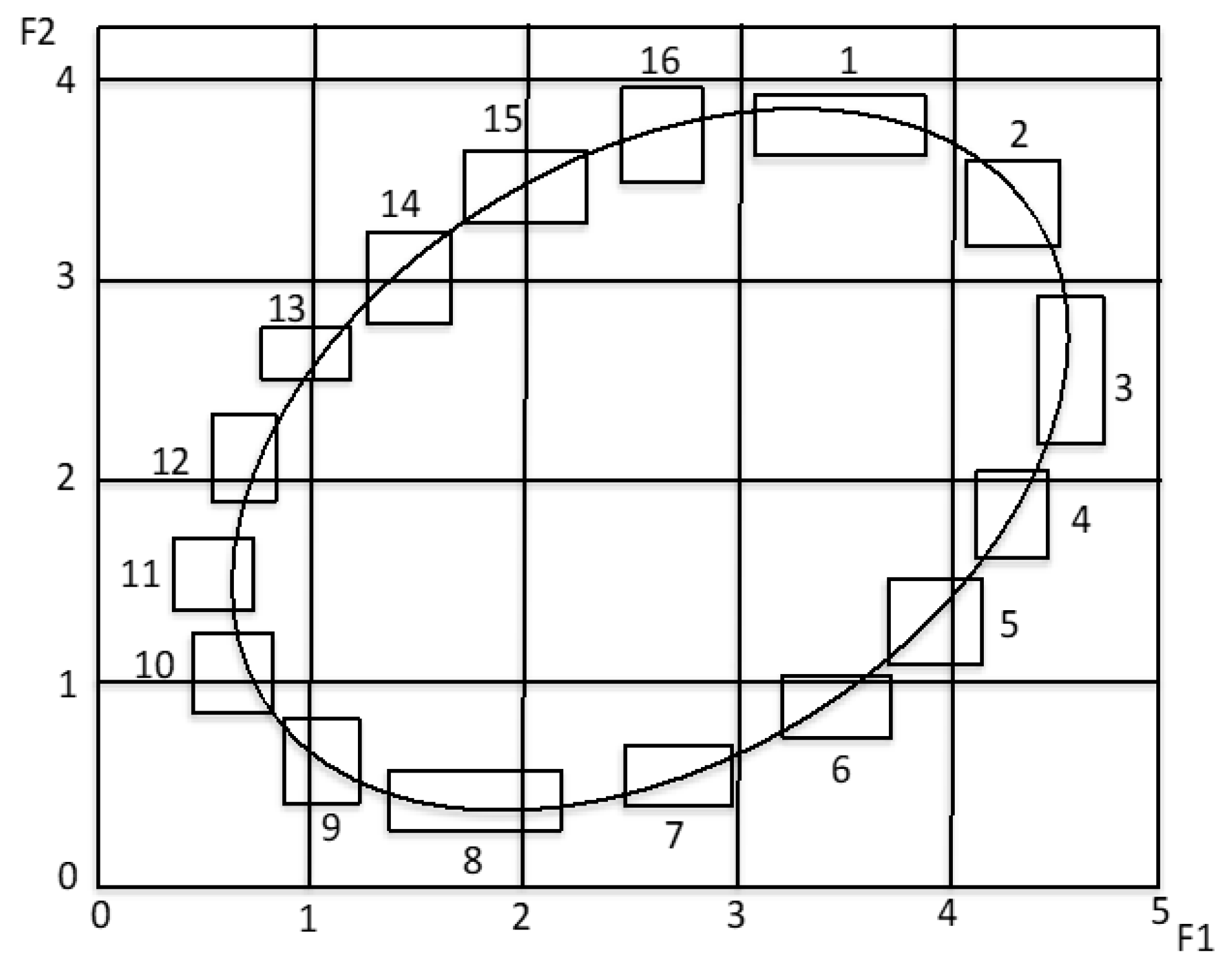
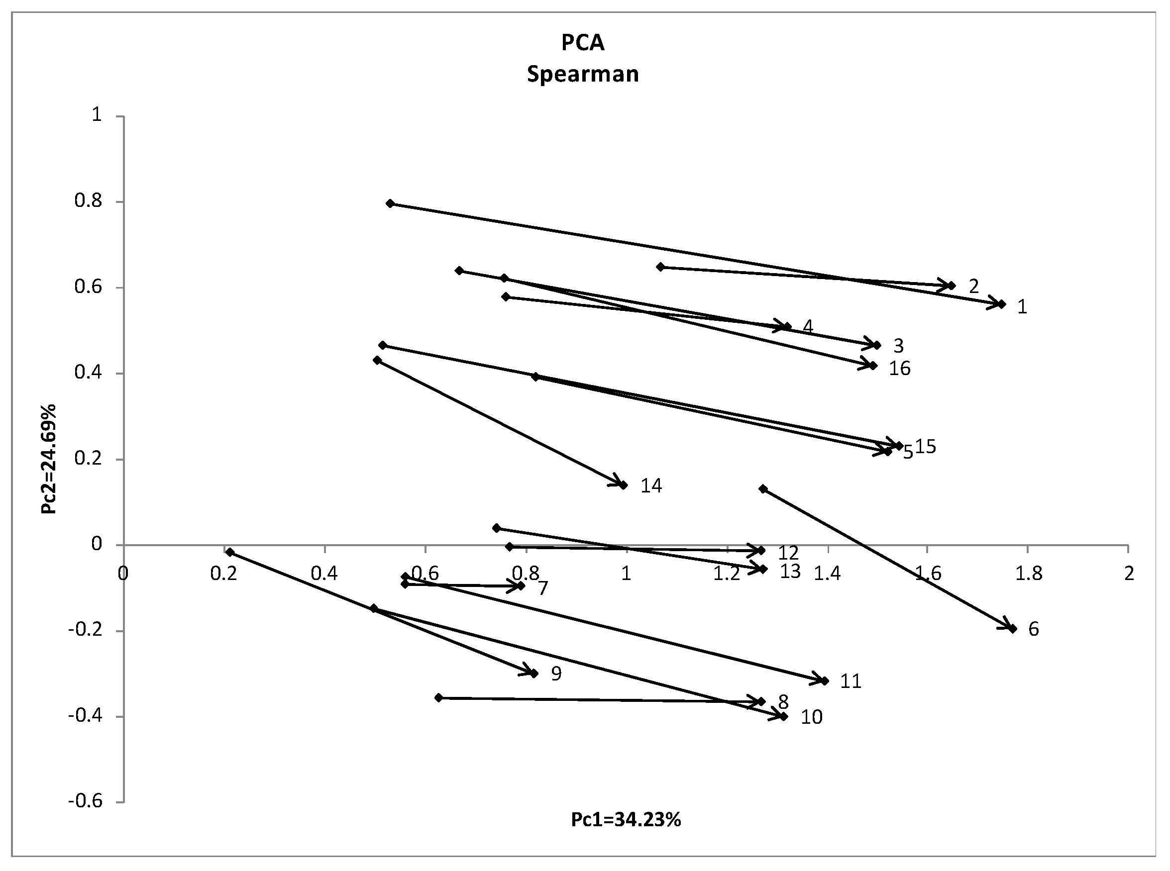
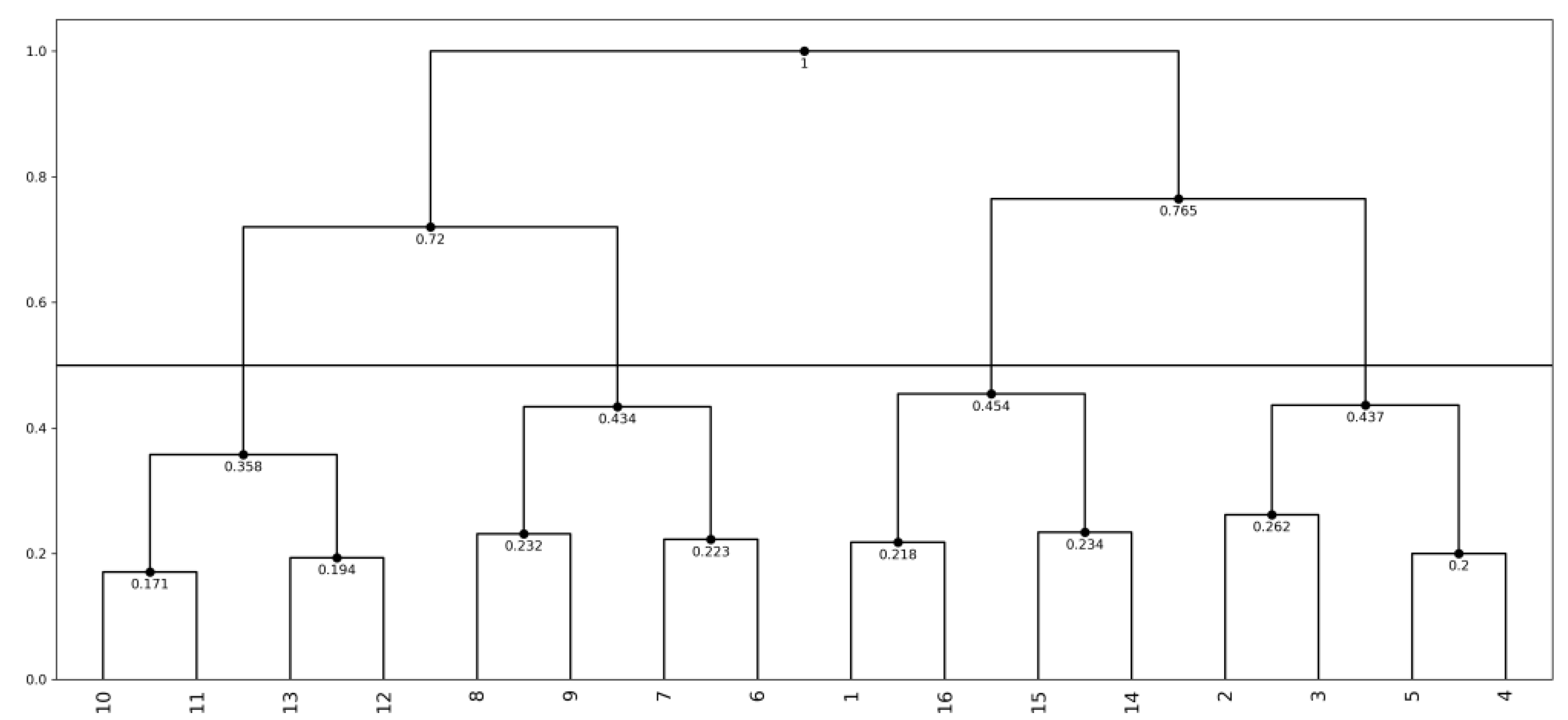
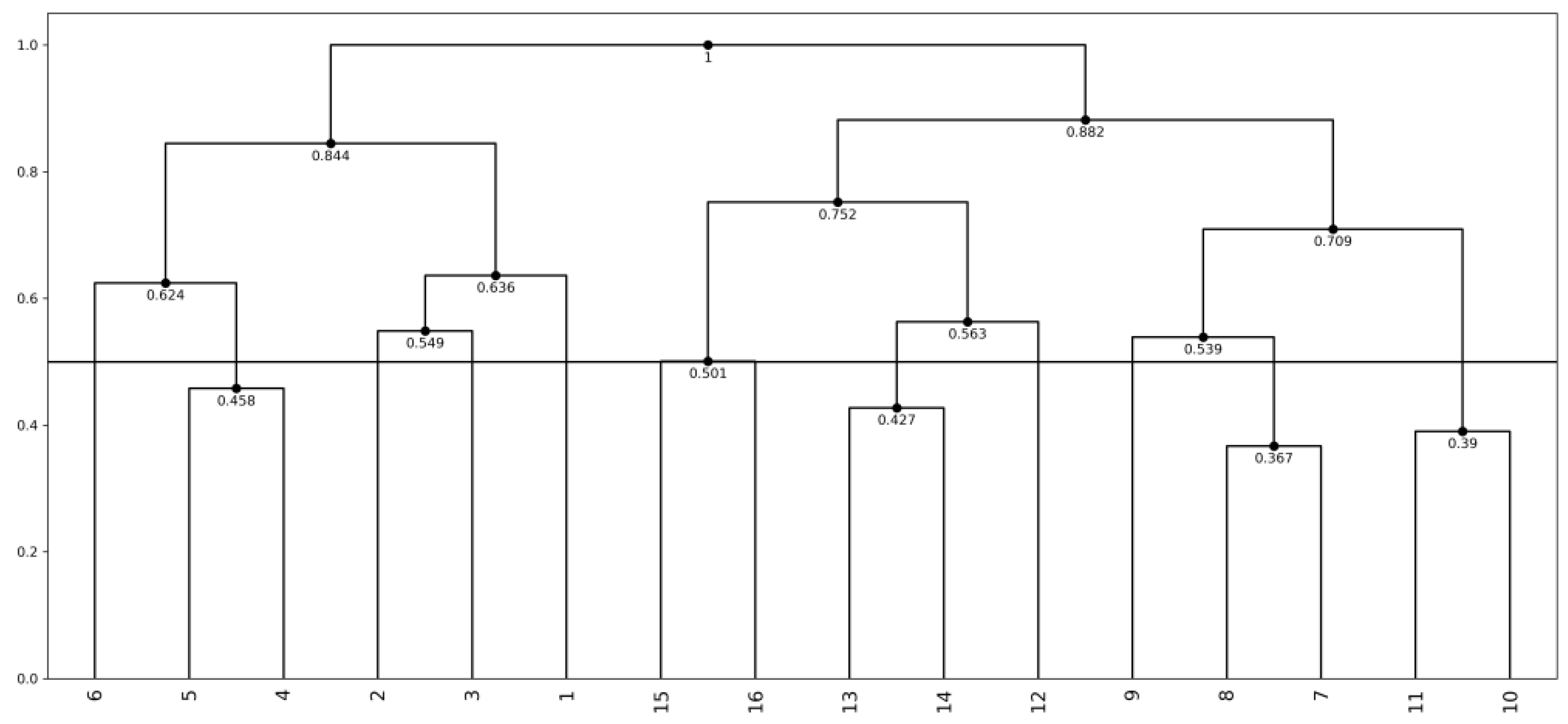
4.2.1. Artificial Data
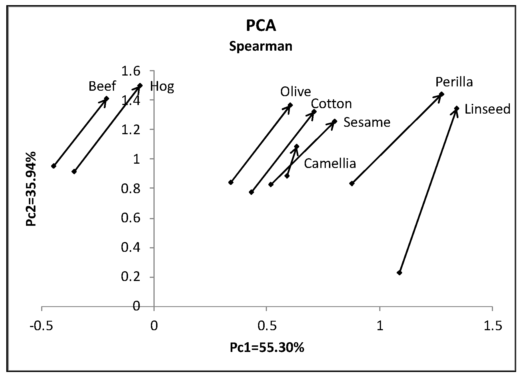
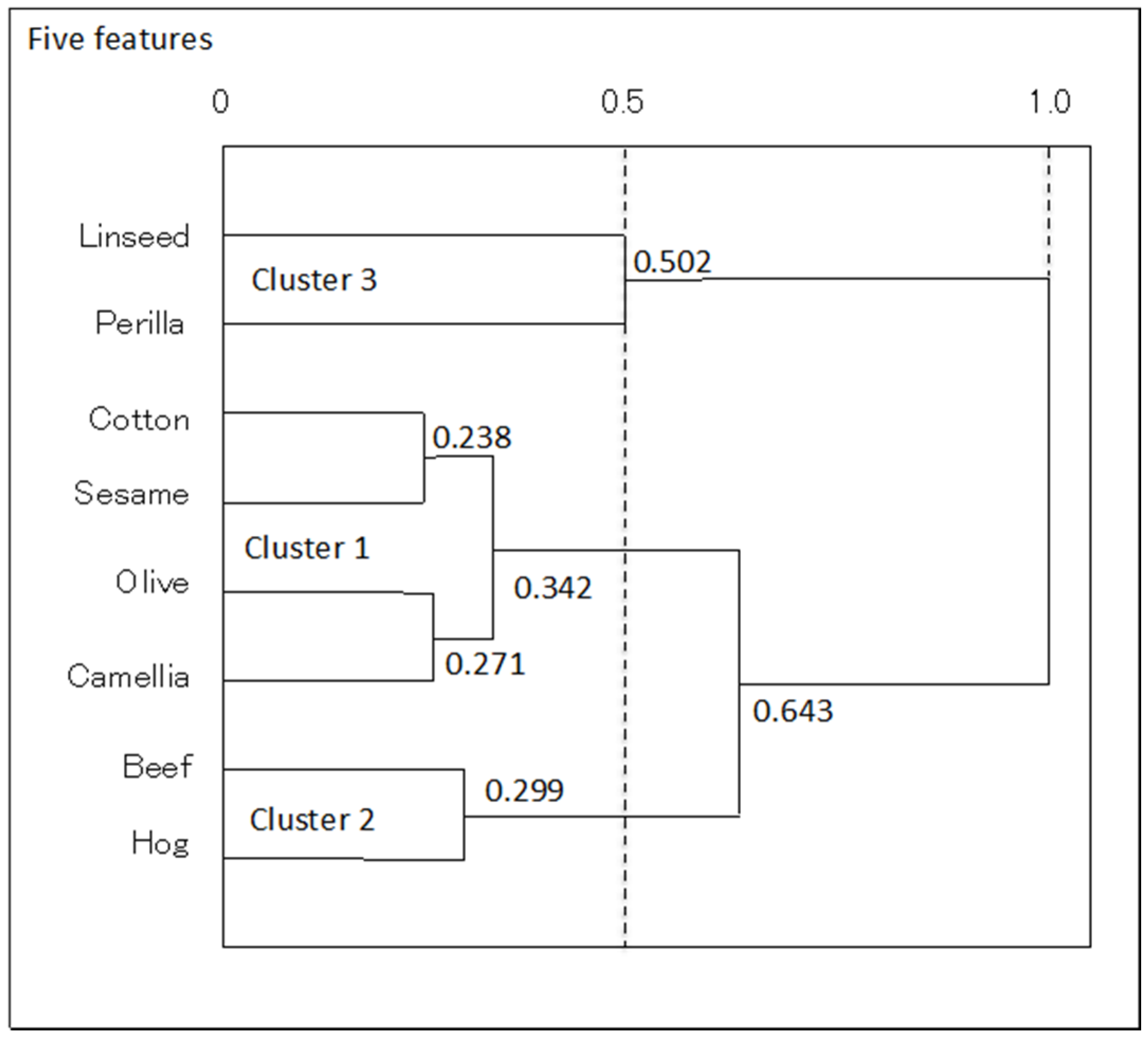
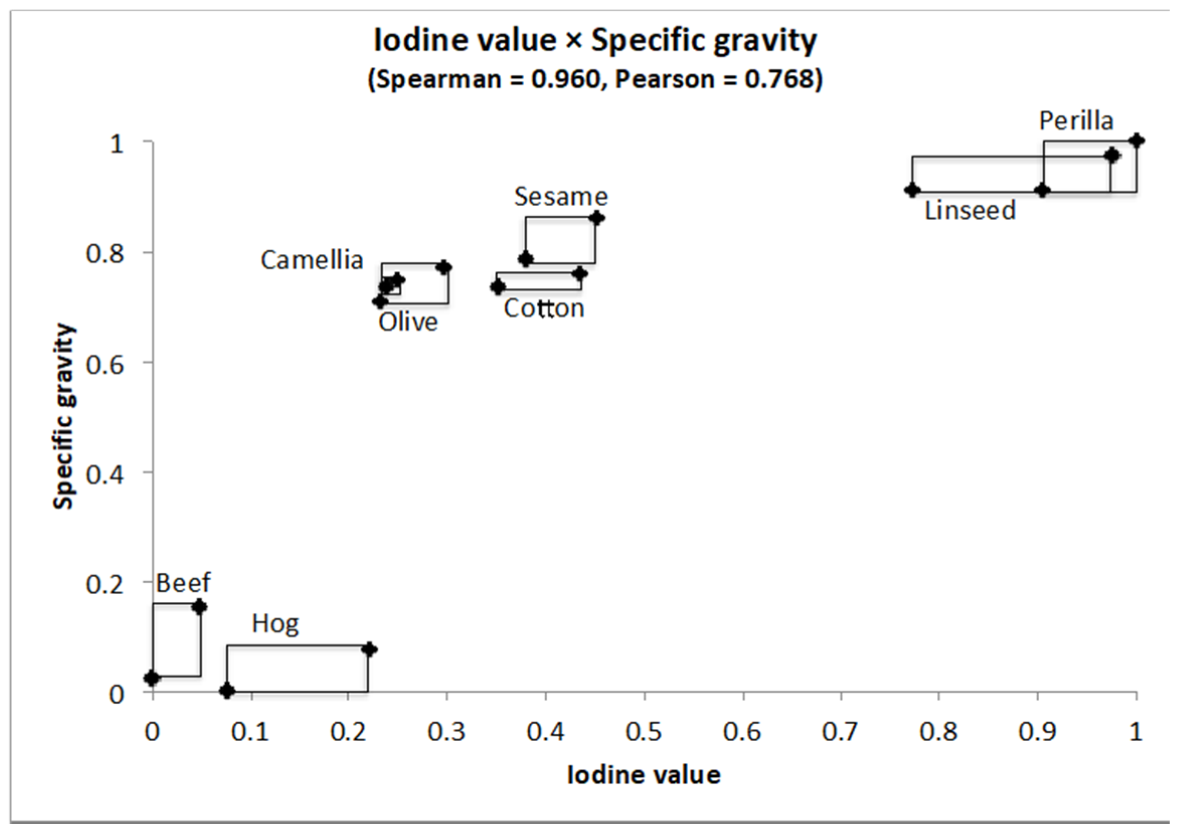
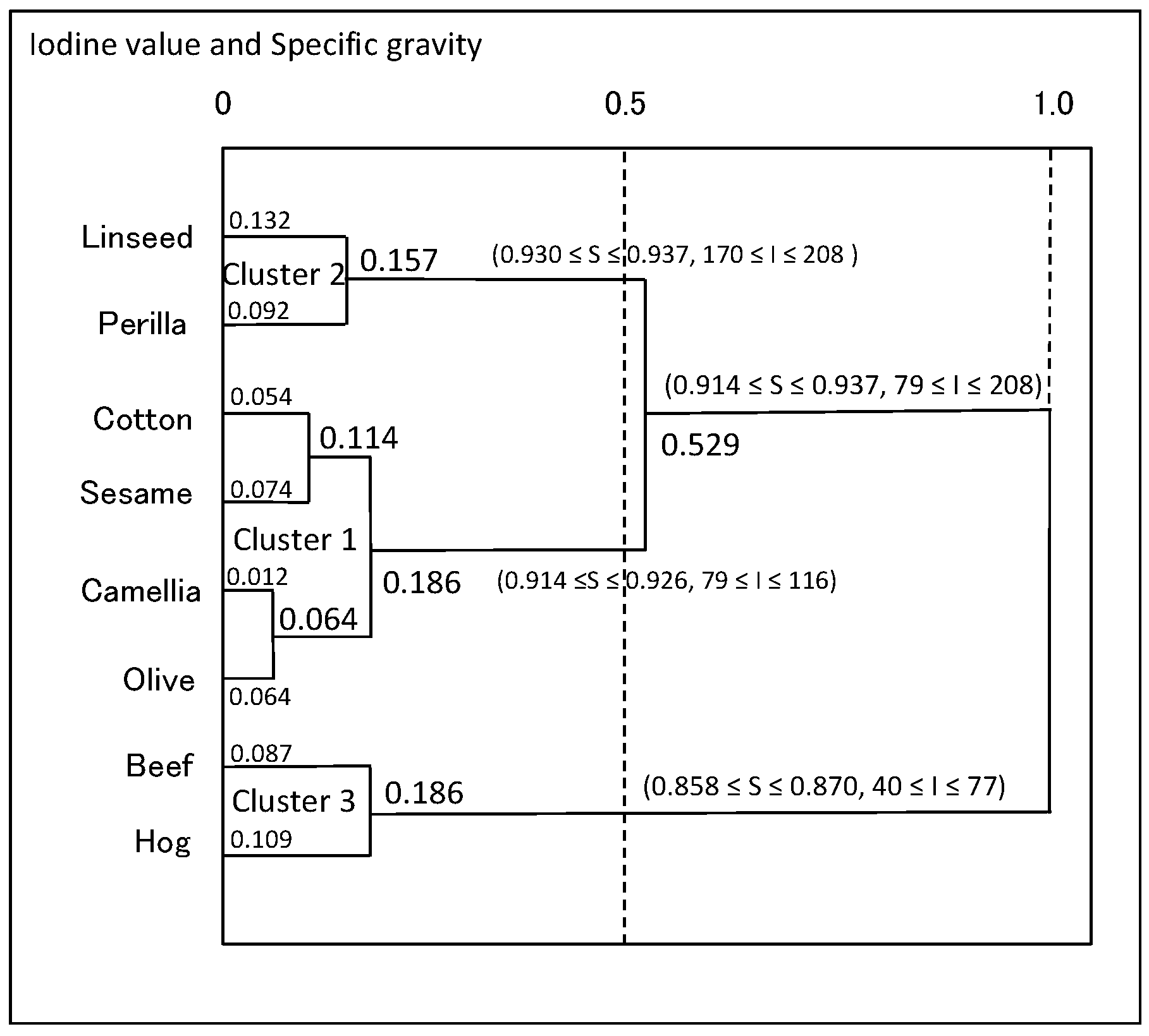
Sixteen small rectangles organize an oval structure in the first two features, F1 and F2, as shown in Figure 5. For each of the sixteen objects, we transform the feature values of F1 and F2 to 0−1 normalized interval values. Then, we select an additional three randomly selected interval values in the unit interval [0, 1] for features F3, F4, and F5. Table 3 summarizes sixteen objects described using five 0−1 normalized interval valued features. It should be noted that usual numerical data is regarded as a special type of interval data, i.e., null interval.
Figure 6 shows the result using the quantile method of PCA (Ichino [13]). Each numbered arrow line connects the minimum and the maximum quantile vectors and describes the corresponding rectangular object. The oval structure embedded in the first two features cannot be reproduced in the factor plane. Any well-known correlation criterion fails to capture the embedded oval structure.
Figure 7 is the dendrogram based on the compactness for the first two features. It is clear that each cluster grows up along the oval structure of Figure 5. Our HCC generates eight comparably sized rectangles along the oval structure, then generates four rectangles, and so on. On the other hand, Figure 8 is the dendrogram for the given five features. We can also recognize the fact that each cluster grows up again along the oval structure of Figure 5 in spite of the addition of three useless features.
Table 4 summarizes the average compactness for each feature in each step of hierarchical clustering. For example, in Step 1, our HCC generates a larger rectangle using objects 10 and 11. Then, for each feature, we recalculate the average side lengths of 15 rectangles including an enlarged rectangle. The result is the second row in Table 4. We repeat the same procedure for succeeding clustering steps. Until step 13, i.e., the number of clusters are three, the importance of the first two features are valid. We clarify this fact by bold format numbers. In many steps, the values of average compactness of features F1 and F2 are sufficiently small compared to the middle point value 0.5. On the other hand, the values of average compactness for the other three features increases rapidly exceeding the middle point 0.5. Thus, we conclude that the first two features are robustly informative through the clustering process. The proposed method could detect our oval structure embedded in five dimensional interval-valued data as a geometrically thin structure. In the following, we use the middle point 0.5 as a criterion whether the average compactness is small or large.

4.2.2. Oils Data

The data in Table 5 describes six plant oils, linseed, perilla, cotton, sesame, camellia, and olive, and two fats, beef and hog, using five interval valued features: specific gravity, freezing point, iodine value, saponification value, and major acids.
The result of PCA in Figure 9 and the dendrogram in Figure 10 show three explicit clusters (linseed, perilla), (cotton, sesame, olive, camellia), and (beef, hog). Table 6 summarizes the values of the average compactness for each feature in each clustering step. As clarified by bold format numbers, the most robustly informative feature is Specific gravity and then Iodine value until Step 5 obtaining three clusters. In the initial step, major acids exceeds our basic criterion 0.5.
Figure 11 is the scatter diagram of the oils data for the selected two robustly informative features. This figure shows again three distinct clusters (linseed, perilla) and (cotton, sesame, camellia, olive), and (beef, hog). They exist in locally limited regions and they organize again a geometrically thin structure with respect to the selected features. Figure 12 shows the dendrogram with concept descriptions of clusters with respect to Specific gravity and Iodine value. This dendrogram clarifies two major clusters, Plant oils and Fats, addition to three distinct clusters, and the compactness takes smaller values compared to the dendrogram in Figure 10.
We should note that our exploratory method to analyze distributional data depends only on the compactness for each feature and combined features. In other words, the measure of feature effectiveness, the measure of similarity between objects and/or clusters, and the measure of cluster quality are based on the same simple notion of the concept size.

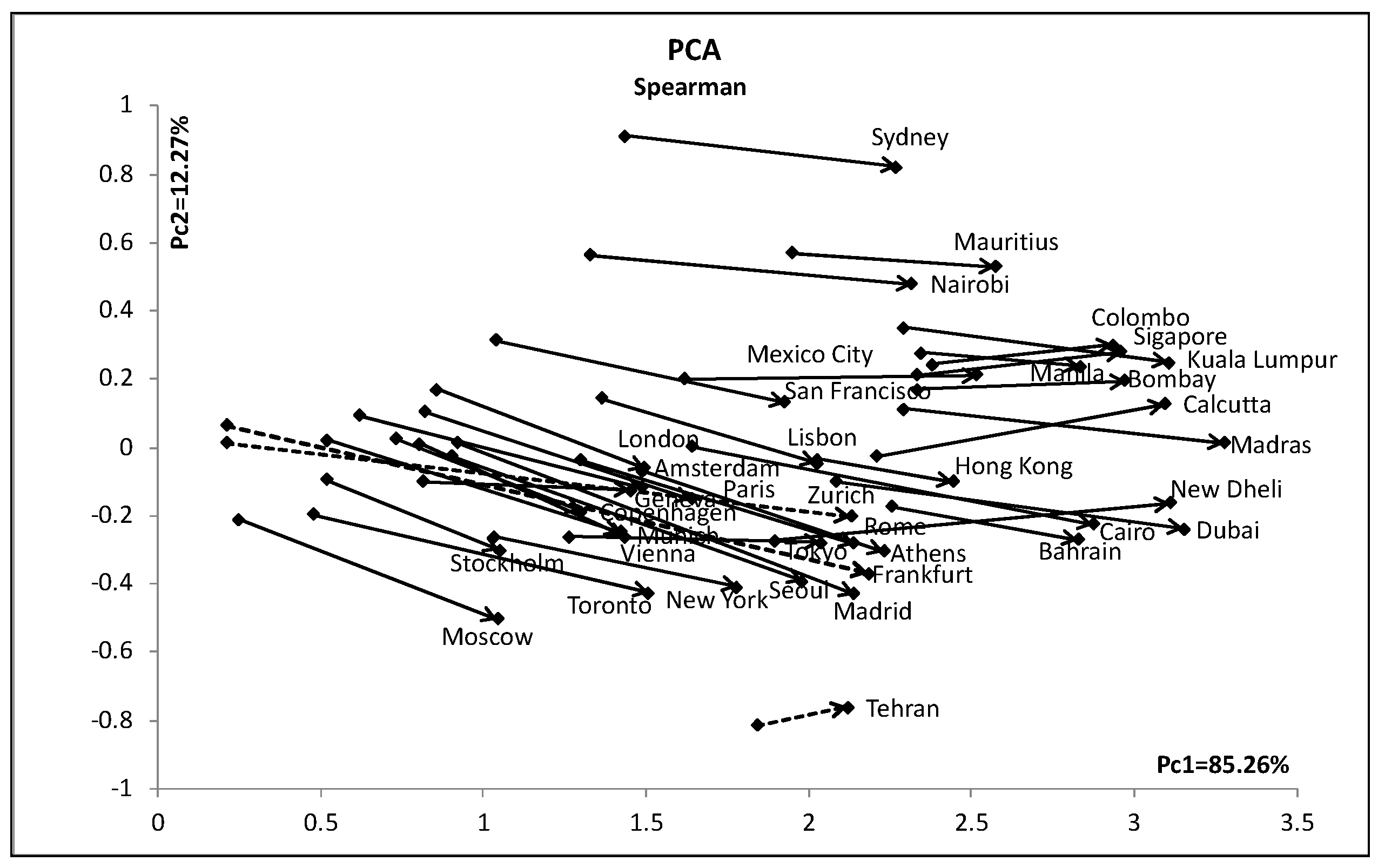
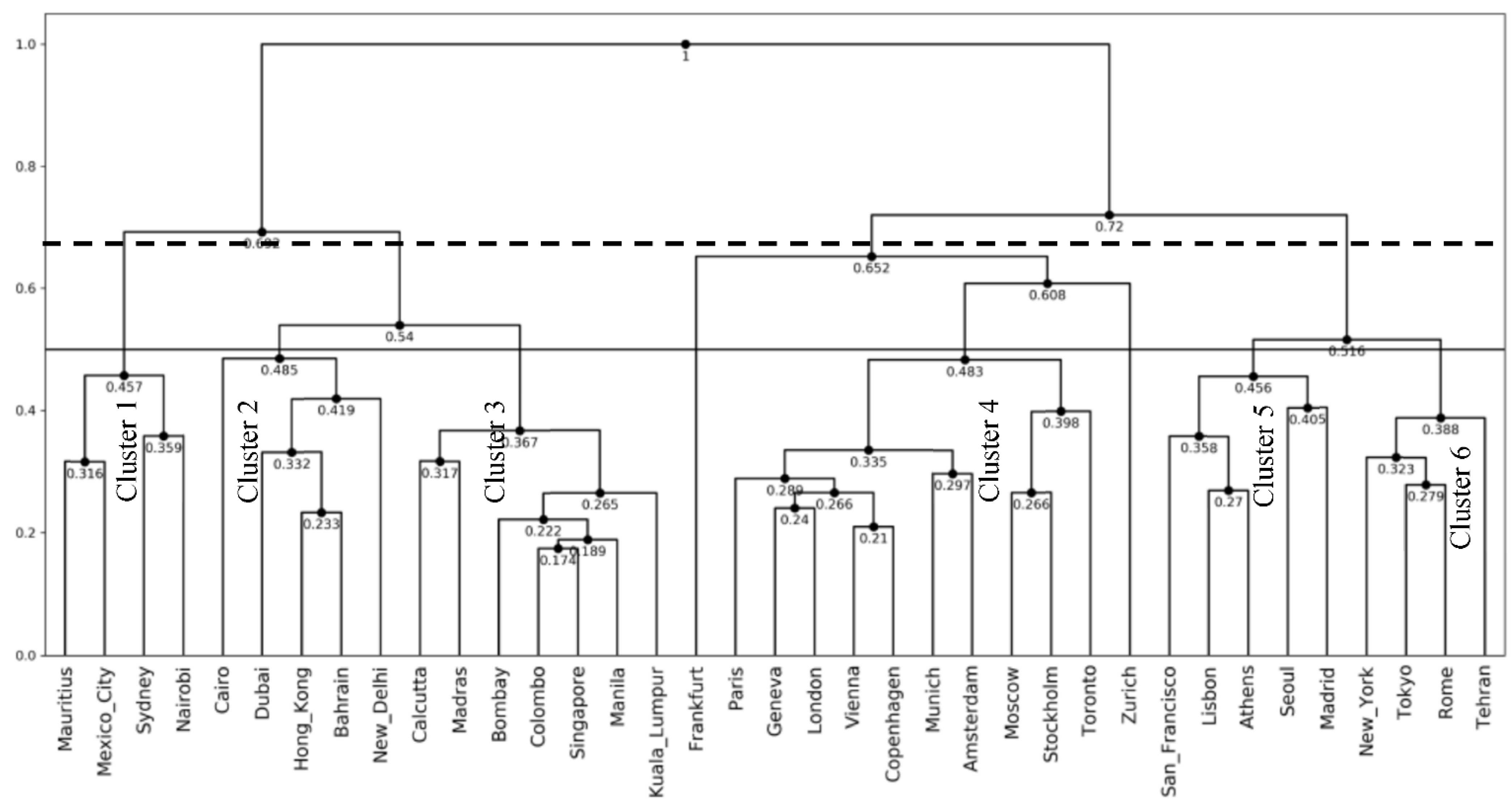
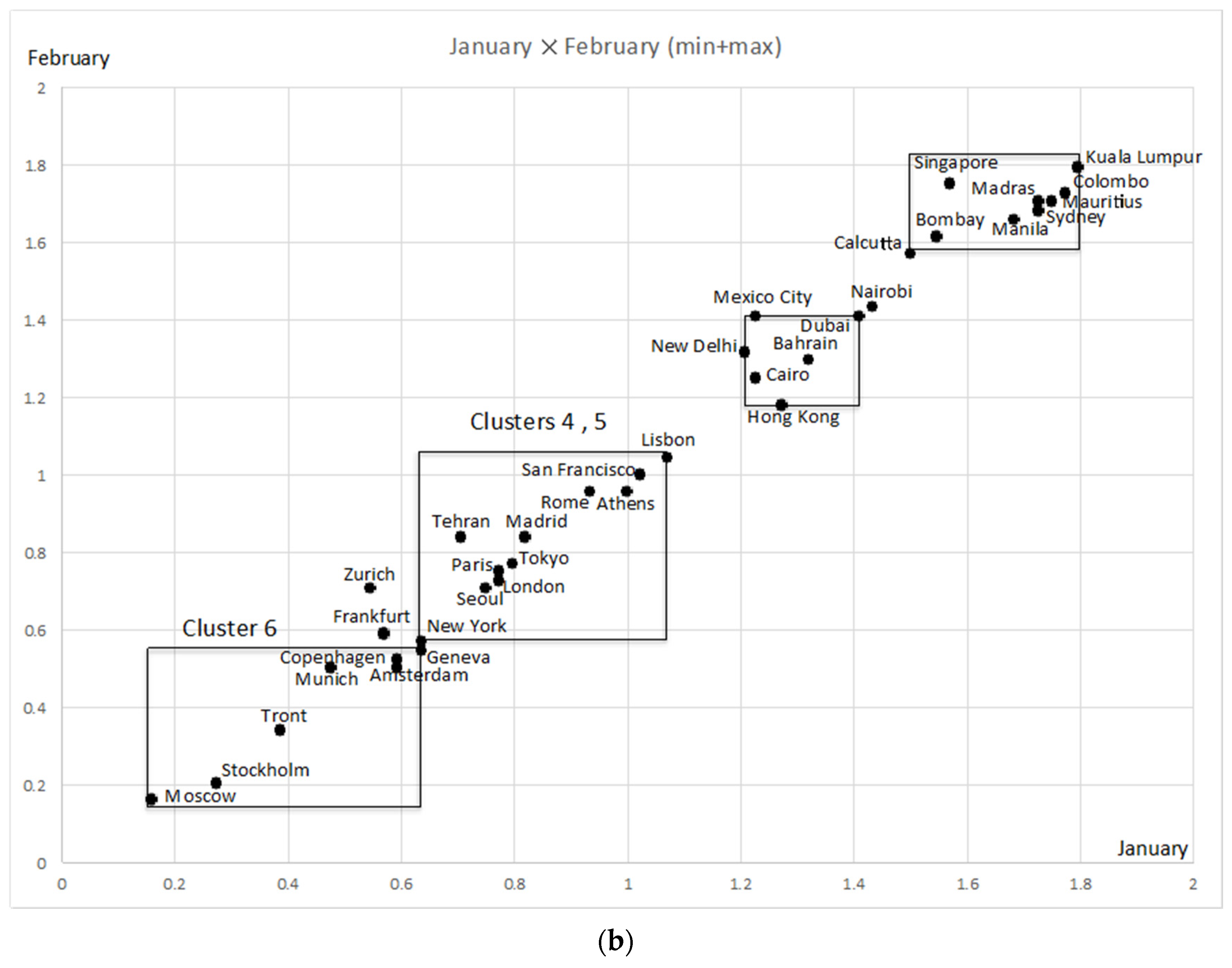
4.3. Analysis of City Temperature Data

De Carvalho and De Souza [10] used this temperature data in their dynamical clustering methods. In this data, 12 interval-valued features describe 37 selected cities. The minimum and the maximum temperatures in degree centigrade determine the interval value for each month. We use 0−1 normalized temperatures for each month, and we obtained the PCA result in Figure 13. In this figure, each arrow line connects from the minimum to the maximum quantile vectors and its length shows the concept size. The first principal component has a large contribution ratio and 37 cities line up from cold (left) to hot (right) in the limited zone between Tehran and Sydney. In this data, we should note that Frankfurt and Zurich have very large concept sizes while Tehran has a very small size compared to other cities.
In Figure 14, we can recognize 6 clusters at cut-point 0.5 except Frankfurt and Zurich. De Carvalho and De Souza [10] obtained four clusters using their dynamical clustering methods. We can find exactly the same clusters by cutting our dendrogram as the dotted line in the figure.
Table 7 shows the average values of the compactness for 12 months at selected clustering steps: 25, 29, 31, 33, and 35. As clarified by bold format numbers, the most informative features are February, then January and May. The feature May is important to recognize Cluster 1, 2, and 3. The scatter diagram of Figure 15a shows this fact explicitly, where we used the sum of the minimum and the maximum temperatures as feature values. Figure 15b is the scatter diagram for January and February. This figure describes well the mutual relations of Cluster 4, 5, and 6, while the distinctions between Cluster 1, 2, and 3 disappear. We should note that we can reproduce essential structures appearing in the dendrogram by using only three selected informative features.

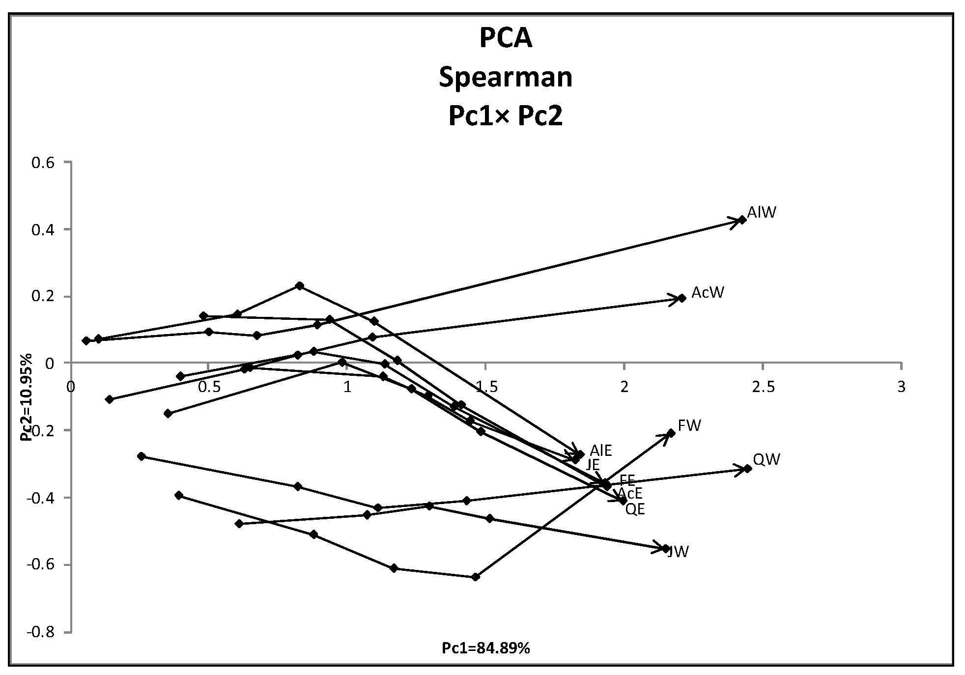
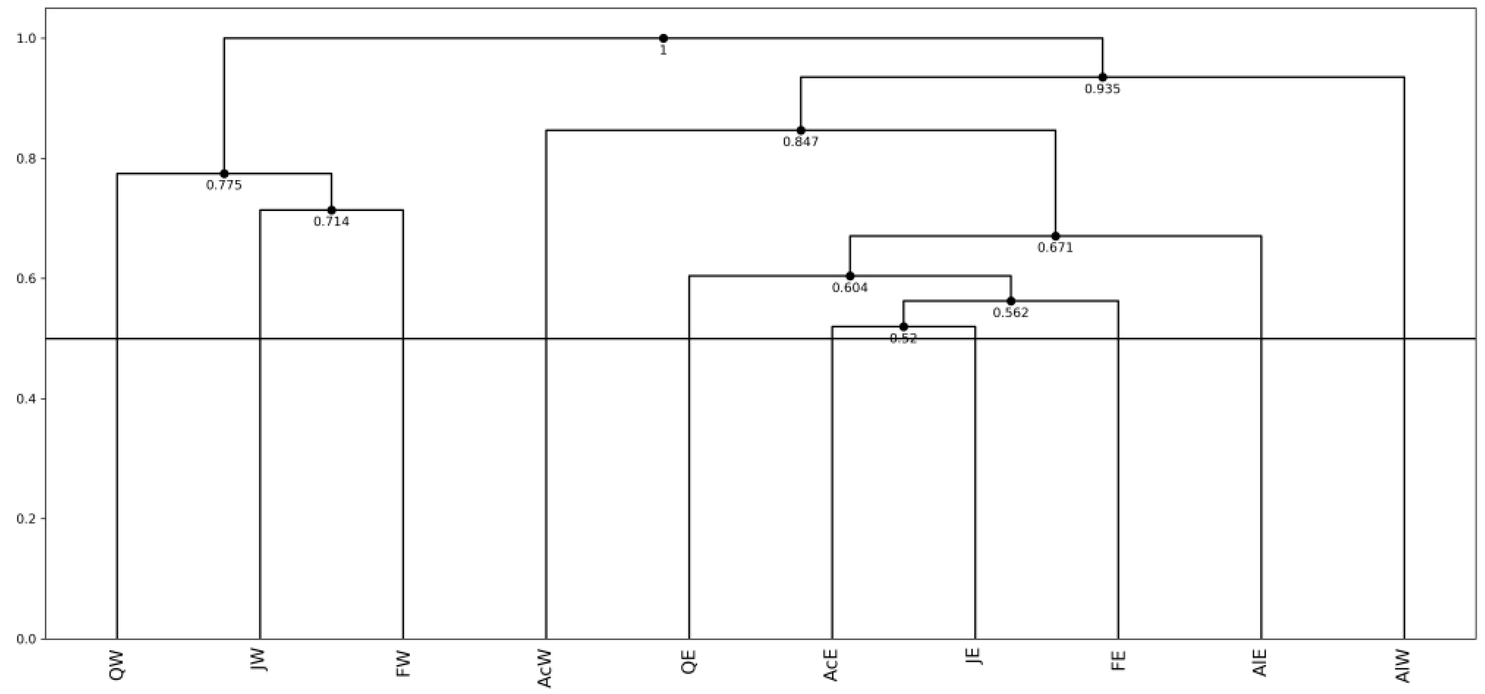
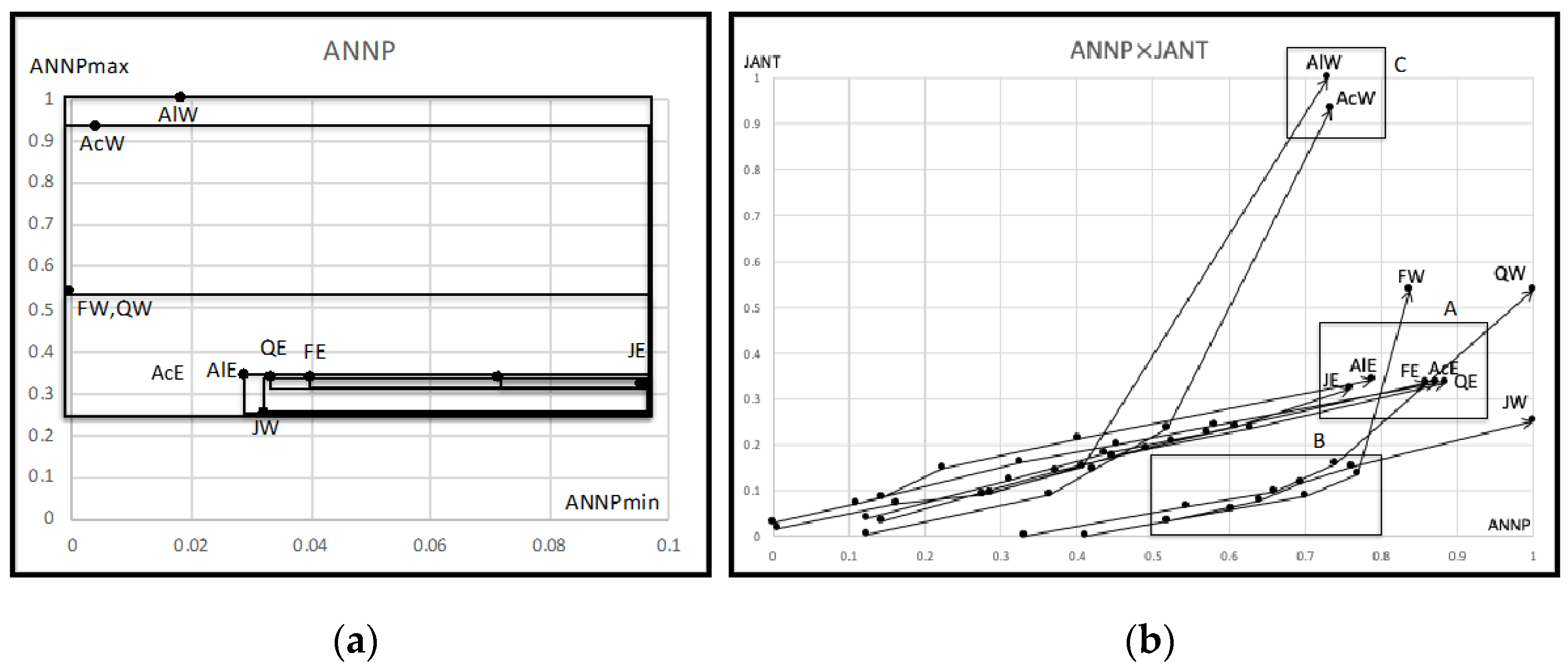
4.4. Analysis of the Hardwood Data

The data is selected from the US Geological Survey (Climate—Vegetation Atlas of North America) [14]. The number of objects is ten and the number of features is eight. Table 8 shows quantile values for the selected ten hardwoods under the feature: (Mean) Annual Temperature (ANNT). We selected the following eight features to describe objects (hardwoods). The data formats for other features F2~F8 are the same as in Table 8.
  • F1: Annual Temperature (ANNT) (°C);
  • F2: January Temperature (JANT) (°C);
  • F3: July Temperature (JULT) (°C);
  • F4: Annual Precipitation (ANNP) (mm);
  • F5: January Precipitation (JANP) (mm);
  • F6: July Precipitation (JULP) (mm);
  • F7: Growing Degree Days on 5 °C base ×1000 (GDC5);
  • F8: Moisture Index (MITM).
We use quartile representation by omitting 10% and 90% quantiles from each feature in order to assure the monotone property of our compactness measure. As a result, our hardwood data is histogram data of the size (10 objects) × (8 features) × (5 quantile values). Table 9 shows a part of our 0−1 normalized hardwood data, where five 8-dimensional quantile vectors describe each hardwood.
Figure 16 is the result of PCA using the quantile method. Four line segments connecting from 0% to 100% quantile vectors in the factor plane represent each hardwood. East hardwoods have similar shapes, while west hardwoods show significant differences in the last line segments connecting from 75% to 100% quantile vectors. We can recognize three clusters, (Acer West, Alnus West), (five east hardwoods), and (Fraxinus West, Juglans West, Quercus West), in this factor plane.
Figure 17 is the result of our HCC for eight features represented by four equiprobability bins. Ten hardwoods, especially AcW and AlW, have very large concept sizes exceeding our simple criterion 0.5. As a result, we have two major chaining clusters:
((((((AcE, JE)FE)QE)AlE)AcW)AlW) and ((FW, JW)QW).
Table 10 shows the average compactness of each feature in each clustering step. As clarified by bold format numbers, the most informative feature is ANNP then JULP. Figure 18a shows the nesting structure of rectangles spanned by ten hardwoods with respect to the minimum and the maximum values of ANNP. Another representation of the structure is:
((((((((JE,AcE)FE)QE)JW)AlE)(FW,QW))AcW)AlW).
Juglans West is merged to the cluster of east hardwoods. From step 8 of Table 10 and Figure 17, we see that JANT is important to separate the cluster (FW, JW, QW) from the other cluster. In fact, we have the scatter diagram of Figure 18b with respect to ANNP and JANT. This scatter diagram is very similar to the PCA result in Figure 16. Figure 18b suggests also the cluster descriptions using three rectangles A, B, and C. Rectangles A and C include the maximum quantile vectors of (AcW, AlW) and five east hardwoods, respectively. Rectangle B includes 25%, 50%, and 75% quantile vectors of (FW, JW, QW). They clarify the distinctions between three clusters.

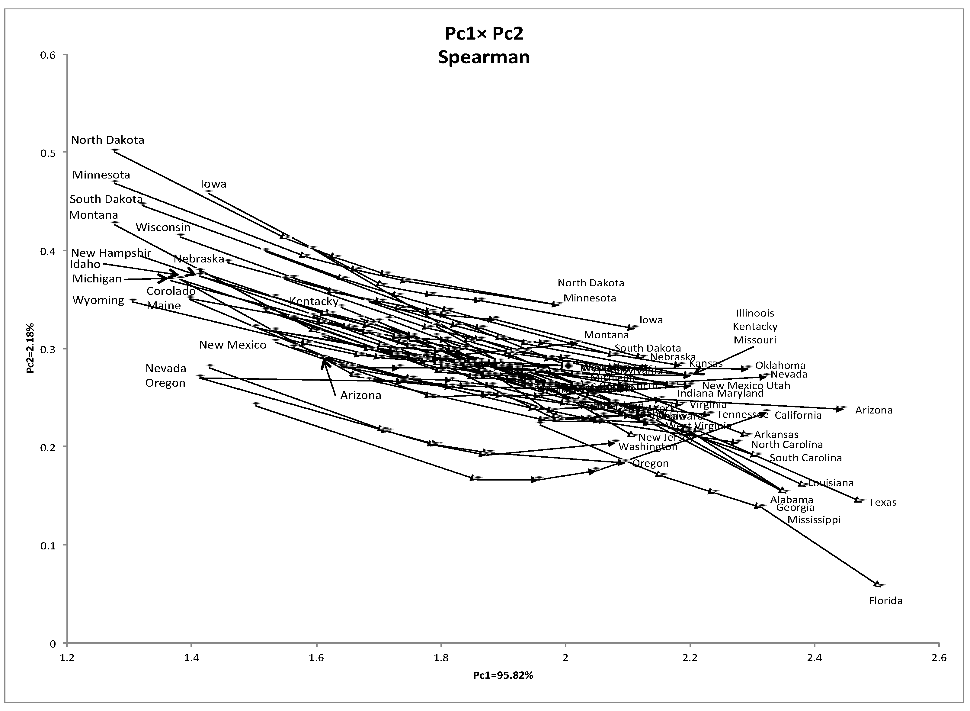
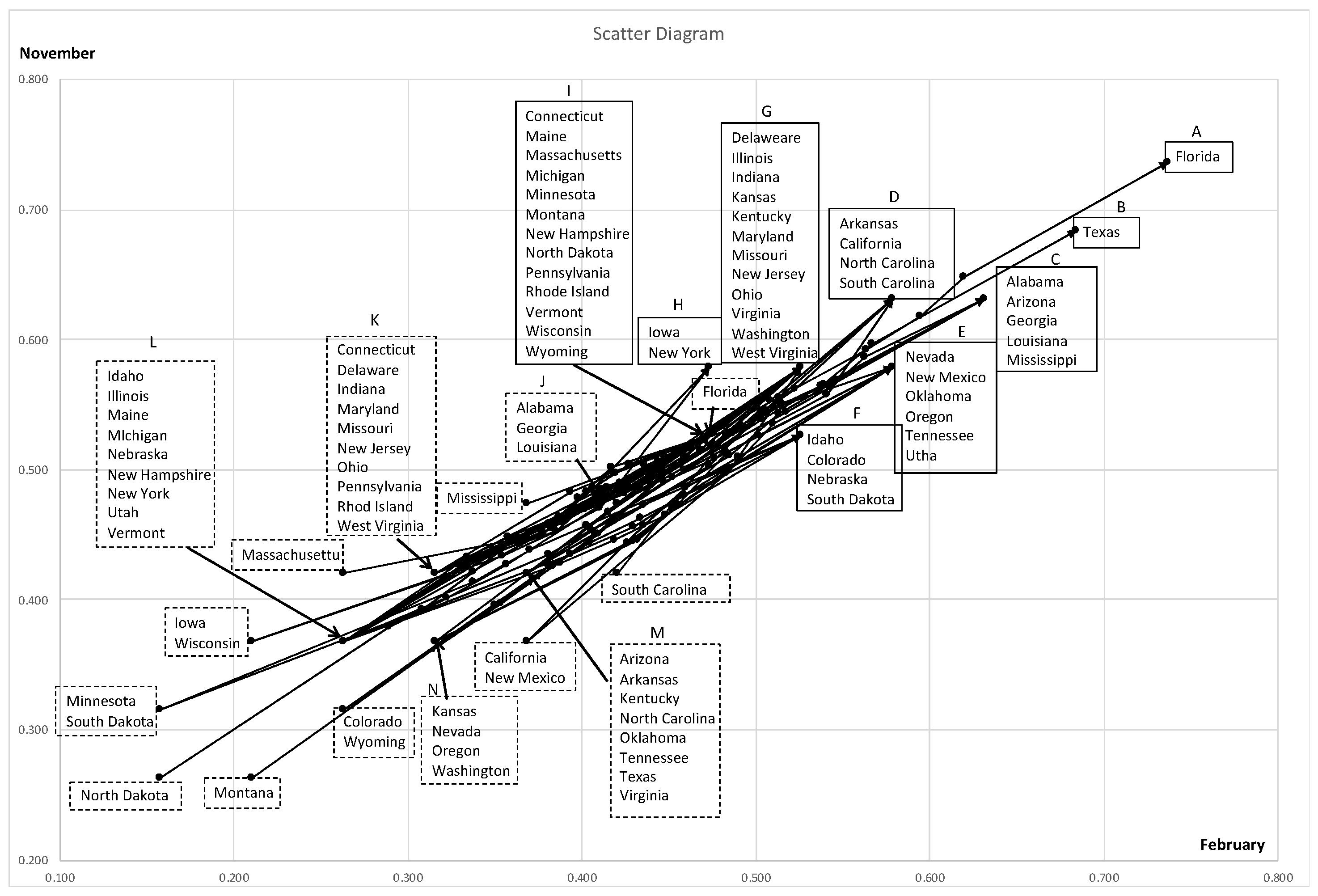
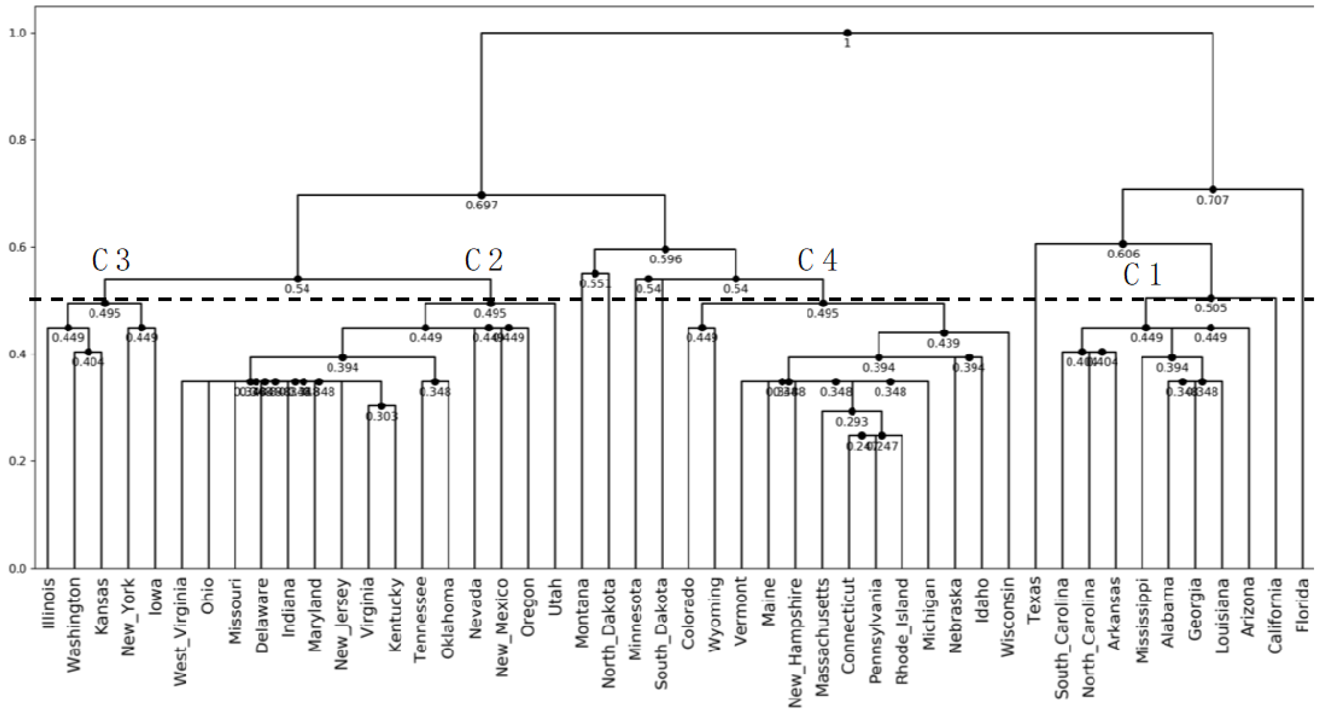
4.5. Analysis of the US Weather Data

We analyze a climate data set [National Data Center (2014)]. The dataset contains sequential monthly “time bias corrected” average temperature data for 48 states of USA (Alaska and Hawaii are not represented in the data set). Years from 1895 to 2009 are used for comparison purposes. We use 0, 25, 50, 75, and 100% quantiles to describe the temperature each month for each of the 48 states. Therefore, five 12-dimensional quantile vectors describe each state.
In the PCA result of Figure 19, each line graph connecting five quantile vectors describes the corresponding state weather. The first principal component has a very large contribution ratio and 48 distributions line up in a narrow zone of the factor plane. Figure 20 is the dendrogram for 12 months. By cutting the dendrogram at the compactness 0.65, we recognize five major clusters except Arizona, California, and Nevada. These clusters include the following sub-clusters having small compactness less than 0.5.
(1)
Alabama, Mississippi, Georgia, and Louisiana;
(2)
Connecticut, Rhode Island, Massachusetts, Pennsylvania, Delaware, New Jersey, and Ohio;
(3)
Indiana, West Virginia, and Virginia:
(4)
Kentucky, Tennessee, and Missouri;
(5)
Arkansas and South Carolina;
(6)
Maine, New Hampshire, and Vermont.
Irpino and Verde [9] applied the Ward’s method using their Wasserstein-based distance to the US state weather data and found five clusters. As noted in Section 3.2, dissimilarity between objects and/or clusters and the compactness of objects and/or clusters are different notions. Nevertheless, sub-clusters (1) and (6), for example, appear in both methods. Furthermore, (North Dakota, Minnesota) and (Oregon, Washington) have very similar distributions. Then, in a distance-based approach, these pairs are merged in very early stages. On the other hand, their compactness is larger than many other states, and thus, the compactness delayed their merging steps until later. However, two different methods show similar behavior for (Oregon, Washington) but different behavior for (North Dakota, Minnesota) in the dendrograms.
Table 11 is the average compactness for each feature in selected clustering steps. As clarified by bold format numbers, February and November are the most robustly informative features. Figure 21 is the scatter diagram of 48 states and is similar to the PCA result in Figure 19. All line graphs exist in a narrow region from “cold” to “warm” with respect to February and November. Many states share the minimum and/or the maximum quantile vectors. For example, Alabama, Georgia, and Louisiana share the maximum quantile vector as noted in box C, and the minimum quantile vector as box J, etc. The value of compactness is directly linked to the span of the minimum and the maximum quantile vectors under the assumption of equal bin probabilities. As a result, we have the dendrogram of Figure 22.
Under the cut point 0.5, four major clusters, C1~C4, are obtained. Six sub-clusters found in Figure 20 are reproduced in the dendrogram using two features. Sub-cluster (2) obtained in Figure 20 was divided into two smaller sub-clusters (Connecticut, Pennsylvania, Rhode Island, and Massachusetts) and (Delaware, New Jersey, and Ohio). Each of them was merged into different major clusters C4 and C2, respectively. (Illinois, Washington, Kansas, New York, and Iowa) is newly generated cluster C3. Minnesota, Montana, North Dakota, and South Dakota have very small minimum quantile vectors in Figure 19 and Figure 21. They organized a single cluster in Figure 20, while they organized two isolated clusters (Montana, North Dakota) and (Minnesota, South Dakota) with the compactness exceeding 0.5 in Figure 22. We should note that the values of compactness of sub-clusters in Figure 22 are less than those values of the same sub-clusters in Figure 20.
Figure 23 is the scatter diagram of eleven distributions including four major clusters and seven outliers. Each bin-rectangle for a cluster is overlapped with bin-rectangles of other clusters and with remaining states. However, the distinctions between clusters and other states are clear from the maximum quantile vectors and/or the minimum quantile vectors. In other words, we can explain the relationships between eleven distributions by using their mutual positions of the maximum and/or the minimum quantile vectors.

5. Discussion

This paper presented an exploratory hierarchical method to analyze histogram-valued symbolic data using unsupervised feature selection. We described each histogram value of each object and/or cluster using a predetermined number of equiprobability bins. We defined the notion of the concept size and then the compactness for objects and/or clusters as the measure of similarity for our hierarchical clustering method. The compactness is a multi-role measure to evaluate the similarity between objects and/or clusters, to evaluate the dissimilarity of a cluster against the whole concept in each clustering step, and to evaluate the effectiveness of features in the selected clustering steps. We showed the usefulness of the proposed method using five distributional data sets. In each example, we could have two or three robustly informative features. The scatter diagram and the dendrogram for the selected features reproduced well the essential structures embedded in the given distributional data.
In supervised feature selection for histogram-valued symbolic data, we can use class-conditional hierarchical conceptual clustering in addition to our unsupervised feature selection method.

Author Contributions

Conceptualization and methodology, M.I. and H.Y.; software and validation, K.U.; original draft preparation, M.I. All authors have read and agreed to the published version of the manuscript.

Funding

This work was supported by JSPS KAKENHI (Grants-in-Aid for Scientific Research) Grant Number 25330268. Part of this work has been conducted under JSPS International Research Fellow program.

Conflicts of Interest

The authors declare no conflict of interest.

References

  1. Dy, J.G.; Brodley, C.E. Feature selection for unsupervised learning. J. Mach. Learn. Res. 2004, 5, 845–889. [Google Scholar]
  2. Liu, H.; Motoda, H. Computational Methods of Feature Selection; CRC Press: London, UK, 2007. [Google Scholar]
  3. Miao, J.; Niu, L. A survey on feature selection. Procedia Comput. Sci. 2016, 91, 919–926. [Google Scholar]
  4. Solorio-Fernández, S.; Martínez-Trinidad, J.F.; Carrasco-Ochoa, J.A. A review of unsupervised feature selection methods. Artif. Intell. Rev. 2020, 53, 907–948. [Google Scholar] [CrossRef]
  5. Bock, H.-H.; Diday, E. Analysis of Symbolic Data; Springer: Berlin/Heidelberg, Germany, 2000. [Google Scholar]
  6. Billard, L.; Diday, E. Symbolic Data Analysis: Conceptual Statistics and Data Mining; Wiley: Chichester, UK, 2007. [Google Scholar]
  7. Diday, E. Thinking by classes in data science: The symbolic data analysis paradigm. WIREs Comput. Stat. 2016, 8, 172–205. [Google Scholar] [CrossRef]
  8. Billard, L.; Diday, E. Clustering Methodology for Symbolic Data; Wiley: Chichester, UK, 2020. [Google Scholar]
  9. Irpino, A.; Verde, R. A new Wasserstein based distance for the hierarchical clustering of histogram symbolic data. In Data Science and Classification; Springer: Berlin/Heidelberg, Germany, 2006; pp. 185–192. [Google Scholar]
  10. de Carvalho, F.d.A.T.; De Souza, M.C.R. Unsupervised pattern recognition models for mixed feature-type data. Pattern Recognit. Lett. 2010, 31, 430–443. [Google Scholar] [CrossRef]
  11. Ichino, M.; Yaguchi, H. Generalized Minkowski metrics for mixed feature-type data analysis. IEEE Trans. Syst. Man Cybern. 1994, 24, 698–708. [Google Scholar] [CrossRef]
  12. Ono, Y.; Ichino, M. A new feature selection method based on geometrical thickness. In Proceedings of the KESDA’98, Luxembourg, 27–28 April 1998; Volume 1, pp. 19–38. [Google Scholar]
  13. Ichino, M. The quantile method of symbolic principal component analysis. Stat. Anal. Data Min. 2011, 4, 184–198. [Google Scholar] [CrossRef]
  14. Histogram Data by the U.S. Geological Survey, Climate-Vegetation Atlas of North America. Available online: http://pubs.usgs.gov/pp/p1650-b/ (accessed on 11 November 2010).
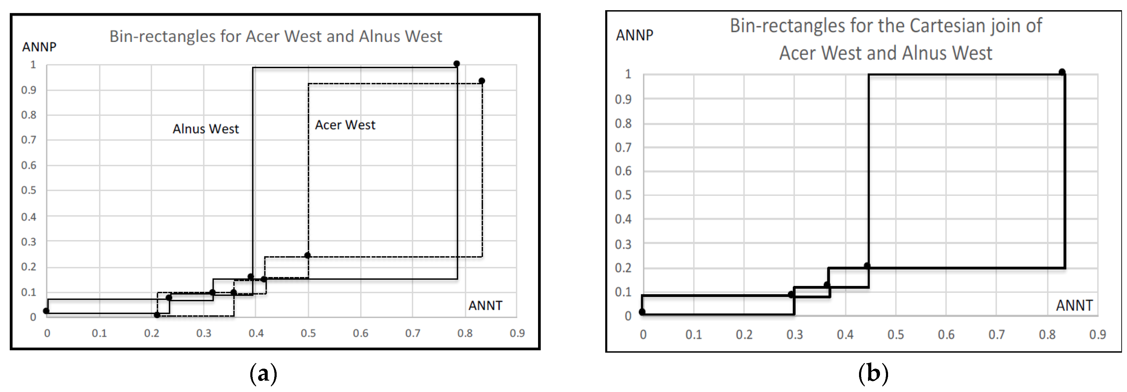
Figure 1. Cumulative distribution function and cut point probabilities.
Stats 04 00024 g001
Figure 2. Representations of objects by bin-rectangles in the quartile case.
Stats 04 00024 g002
Figure 3. Bin-rectangles for two hardwoods and their Cartesian join.
Stats 04 00024 g003
Figure 4. Examples for compactness.
Stats 04 00024 g004
Figure 5. Oval data.
Stats 04 00024 g005
Figure 6. PCA result for oval artificial data.
Stats 04 00024 g006
Figure 7. Dendrogram using the HCC for the first two features.
Stats 04 00024 g007
Figure 8. Dendrogram using the HCC for five features.
Stats 04 00024 g008
Figure 9. PCA result for Oils data.
Stats 04 00024 g009
Figure 10. Dendrogram using HCC for five features.
Stats 04 00024 g010
Figure 11. Scatter diagram using two informative features.
Stats 04 00024 g011
Figure 12. Descriptions using specific gravity and iodine value.
Stats 04 00024 g012
Figure 13. PCA result for city temperature data.
Stats 04 00024 g013
Figure 14. Dendrogram for 12 months.
Stats 04 00024 g014
Figure 15. (a) Cluster descriptions for February and May. (b) Cluster descriptions for January and February.
Stats 04 00024 g015aStats 04 00024 g015b
Figure 16. PCA result for hardwood data.
Stats 04 00024 g016
Figure 17. Results of clustering for hardwoods data (eight features).
Stats 04 00024 g017
Figure 18. Scatter diagrams for the selected informative features.
Stats 04 00024 g018
Figure 19. PCA result for US state weather data.
Stats 04 00024 g019
Figure 20. Dendrogram for 12 months.
Stats 04 00024 g020
Figure 21. The scatter diagram of 48 distributions for February and November.
Stats 04 00024 g021
Figure 22. Clustering result of the US state weather data for February and November.
Stats 04 00024 g022
Figure 23. Scatter diagram of four major clusters and seven outliers.
Stats 04 00024 g023
Table 1. Two hardwoods using quartile representations.
QuantilesANNTANNP
Acer West 00.2110.004
10.3580.091
20.4160.145
30.5000.237
40.8320.932
Alnus West 00.0000.018
10.2340.071
20.3170.092
30.3910.153
40.7841.000
Table 2. The average concept sizes for two hardwoods and their Cartesian join.
Concept SizeANNTANNPAverage
Acer West0.1550.2320.194
Alnus West0.1960.2450.221
Cartesian join0.2080.2490.229
Table 3. Oval artificial data.
F1F2F3F4F5Concept Size
1[0.629, 0.798][0.905, 0.986][0.000, 0.982][0.002, 0.883][0.360, 0.380]0.427
2[0.854, 0.955][0.797, 0.905][0.002, 0.421][0.573, 1.000][0.754, 0.761]0.212
3[0.921, 1.000][0.527, 0.716][0.193, 0.934][0.035, 0.477][0.406, 0.587]0.326
4[0.865, 0.933][0.378, 0.500][0.452, 0.854][0.213, 0.604][0.000, 0.074]0.211
5[0.775, 0.876][0.257, 0.338][0.300, 0.614][0.425, 0.979][0.217, 0.568]0.280
6[0.663, 0.764][0.135, 0.216][0.712, 1.000][0.904, 0.968][0.103, 0.950]0.276
7[0.494, 0.596][0.041, 0.122][0.293, 0.470][0.023, 0.086][0.765, 0.902]0.112
8[0.225, 0.427][0.000, 0.081][0.633, 0.872][0.000, 0.582][0.719, 0.852]0.247
9[0.112, 0.213][0.041, 0.149][0.167, 0.802][0.056, 0.129][0.124, 0.642]0.287
10[0.022, 0.112][0.162, 0.270][0.026, 0.718][0.418, 0.851][0.549, 0.853]0.325
11[0.000, 0.090][0.297, 0.392][0.096, 0.759][0.438, 0.938][0.495, 0.760]0.323
12[0.045,0.112][0.446, 0.554][0.826, 0.962][0.230, 0.755][0.104, 0.189]0.184
13[0.101, 0.202][0.608, 0.676][0.367, 0.570][0.236, 0.684][0.683, 0.930]0.213
14[0.213, 0.292][0.676, 0.811][0.371, 0.381][0.086, 0.305][0.009, 1.000]0.287
15[0.315, 0.438][0.811, 0.919][0.049, 0.585][0.056, 0.891][0.528, 0.881]0.391
16[0.483, 0.562][0.878, 1.000][0.402, 0.609][0.150, 0.769][0.207, 0.732]0.310
Average
CS
0.1030.1050.4150.4410.3150.276
Table 4. Average compactness of each feature in each clustering step.
Clustering StepAverage Compactness
F1F2F3F4F5
00.1030.1050.4150.4410.315
10.1150.1090.4540.4660.330
20.1180.1190.4420.4700.338
30.1280.1280.4750.5010.345
40.1380.1420.5010.5280.386
50.1540.1510.5300.5190.403
60.1710.1580.5320.5640.451
70.1860.1850.5660.6370.519
80.2080.2150.6690.6600.574
90.2390.2510.7440.7440.589
100.2880.2930.7120.7270.692
110.3460.3540.7360.8390.759
120.4380.4430.8600.8820.780
130.4940.5990.9190.9240.906
140.4830.9260.9670.9680.971
151.0001.0001.0001.0001.000
Table 5. Oils data.
Table 5. Oils data.
Specific GravityFreezing PointIodine ValueSaponification v.Major Acids
Linseed[0.930, 0.935][−27, −18][170, 204][118, 196][1.75, 4.81]
Perilla[0.930, 0.937][−5, −4][192, 208][188, 197][0.77, 4.85]
Cotton[0.916, 0.918][−6, −1][99, 113][189, 198][0.42, 3.84]
Sesame[0.920, 0.926][−6,−4][104, 116][187, 193][0.91, 3.77]
Camellia[0.916, 0.917][−21, −15][80, 82][189, 193][2.00, 2.98]
Olive[0.914, 0.919][0, 6][79, 90][187, 196][0.83, 4.02]
Beef[0.860, 0.870][30, 38][40, 48][190, 199][0.31, 2.89]
Hog[0.858, 0.864][22, 32][53, 77][190, 202][0.37, 3.65]
Table 6. Average compactness of each feature in each clustering step.
FeatureAverage Compactness for Each Clustering Step
01234567
Specific gravity0.0660.0800.0910.0990.1140.1310.4751.000
Freezing point0.0900.0990.1540.1780.2040.3380.6311.000
Iodine value0.0900.0950.1090.1370.1850.2220.3391.000
Saponification value0.2020.2240.2540.2830.3270.4050.5601.000
Major acids0.6460.6480.7200.7530.7750.8090.8561.000
Table 7. Average compactness of each feature in selected clustering steps.
StepsAverage Compactness for Several Clustering Steps
Jan.Feb.Mar.Apr.MayJun.Jul.Aug.Sept.Oct.Nov.Dec.
00.1950.1940.2240.2650.2170.2810.3050.2860.2890.2660.2330.194
250.3600.3450.3630.4060.3610.4610.5190.4840.4660.4220.4100.375
290.4090.3890.4260.4900.4140.5440.6090.5550.5160.4560.4430.429
310.4660.4430.4760.5000.4510.5930.6670.6090.5680.5150.4860.476
330.4890.4770.4760.5000.4640.6180.6940.6640.5860.5220.5000.512
350.5800.5680.5830.6450.6560.8530.9840.9690.7970.6620.6080.583
Table 8. The original quantile values for ANNT.
Taxon NameMean Annual Temperature (℃)
0%10%25%50%75%90%100%
ACER EAST−2.30.63.89.214.417.924
ACER WEST−3.90.21.94.27.510.321
ALNUS EAST−10−4.4−2.30.66.115.021
ALNUS WEST−12−4.6−3.00.33.27.619
FRAXINUS EAST−2.31.44.38.614.117.923
FRAXINUS WEST2.69.411.517.221.222.724
JAGLANS EAST1.36.99.112.415.517.621
JAGLANS WEST7.312.614.116.319.422.727
QUERCUS EAST−1.53.46.311.216.419.124
QUERCUS WEST−1.56.09.514.617.919.927
Table 9. A part of the hardwood data using quantile representation.
Taxon NameF1F2F3F4F5F6F7F8
ACER EAST 00.2510.1100.1650.0720.0140.1240.0480.587
10.4060.3260.4160.1630.0590.1970.1670.935
20.5430.4520.5660.2010.1020.2210.2860.967
30.6750.5810.7000.2420.1430.2500.4170.989
40.9140.8720.8130.3360.2480.4910.7981.000
ACER WEST 00.2110.1240.0000.0040.0060.0000.0000.065
10.3580.3640.2130.0910.0800.0510.0710.576
20.4160.4200.2920.1450.1370.0840.1190.728
30.5000.5180.3930.2370.2630.1150.1790.902
40.8320.7340.8280.9320.9230.3540.6551.000
Table 10. Average compactness of each feature in each clustering step.
StepAverage Compactness of Each Feature
ANNTJANTJULTANNPJANPJULPGDC5MITM
00.1610.1600.1780.1150.1130.1330.1800.196
10.2200.2280.2390.1440.1400.1720.2460.242
20.2290.2340.2680.1860.1970.1910.2560.323
30.2380.2430.2820.2020.2170.2030.2680.338
40.2790.2690.3220.2230.2430.2200.2920.358
50.4040.3950.4750.3370.3720.3500.4550.541
60.4900.4720.5700.3880.4280.4010.5250.614
70.6010.5780.6920.5710.5950.5050.6460.739
80.8290.7770.9380.7680.8100.8870.8991.000
Table 11. The average compactness in selected clustering steps.
StepAverage Compactness of Each Feature in Selected Clustering Steps
JanFebMarAprMayJuneJulyAugSeptOctNovDec
00.4600.3960.5160.4520.5280.4860.5580.5710.5000.4550.3840.447
50.4700.4040.5290.4620.5430.5000.5810.5910.5120.4680.3950.455
100.4820.4110.5390.4770.5610.5180.6000.6050.5220.4770.4040.462
150.4940.4330.5450.4890.5760.5300.6240.6180.5350.4850.4180.471
200.5070.4450.5540.4950.5890.5480.6430.6210.5480.4950.4330.476
250.5260.4620.5710.5160.6160.5510.6610.6350.5650.5090.4490.488
300.5440.4800.5760.5160.6300.5740.6890.6440.5830.5240.4570.500
350.5620.5030.5960.5270.6540.5900.7230.6620.6150.5490.4790.513
400.6120.5450.6410.6070.7500.6670.7750.7500.6880.5890.5280.542
410.6290.5450.6430.6120.7620.6670.8000.7710.7140.6120.5400.556
420.6500.5760.6460.6190.7780.6670.8330.7670.7220.6190.5370.574
430.6600.6000.6500.6290.8000.7000.8800.8000.7670.6290.5560.600
440.7000.6140.6880.6430.8330.7080.9000.8000.7920.6790.5830.639
450.7330.6670.7080.6670.8890.7220.8670.8000.7780.6670.6300.667
460.8000.6820.7500.7860.9170.7500.9000.9000.8330.7860.7220.722
Publisher’s Note: MDPI stays neutral with regard to jurisdictional claims in published maps and institutional affiliations.

