Article

Weighted Log-Rank Statistics for Accelerated Failure Time Model

Department of Mathematics, Illinois Weseyan University, Bloomington, IL 617071, USA
Stats 2021, 4(2), 348-358; https://doi.org/10.3390/stats4020023
Submission received: 23 March 2021 / Revised: 28 April 2021 / Accepted: 30 April 2021 / Published: 3 May 2021
(This article belongs to the Special Issue Survival Analysis: Models and Applications)

Abstract

:
This paper improves the sensitivity of the G ρ family of weighted log-rank tests for the accelerated failure time model, accommodating realistic alternatives in survival analysis with censored data, such as heavy censoring and crossing hazards. The procedures are based on a weight function with the censoring proportion incorporated as a component. Extensive simulations show that the weight function enhances the performance of the G ρ family, increasing its sensitivity and flexibility. The weight function method is illustrated with an example concerning vaginal cancer.

1. Introduction

An important issue in survival analysis is to analyze differences of two samples, especially when data are possibly censored. An example includes evaluation of treatment effects in randomized clinical trials. In such treatment outcome studies, patients are randomized into groups, one receiving a new treatment and the other receiving a fake treatment (placebo). They can be statistically compared over time to reveal effects of the new treatment. For these kinds of studies, the Cox proportional hazards model would be the usual choice of a modeling tool in the presence of censoring. It is, in fact, the most popular approach over other models that can be used in the analysis of survival data. This is primarily because it does not assume a distribution on the baseline hazard. This model, however, assumes hazard functions of two groups that are proportional over the course of study. The assumption of proportional hazards is often violated for the entire study, although the assumption holds for a short period of time, and this restricts its usage in practice. The accelerated failure time (AFT hereafter) model does not require the proportionality assumption. Furthermore, it has a simple structure in which the lifetime is accelerated or decelerated by a scale factor. For those reasons, the AFT would be an appealing alternative model to the Cox proportional hazards model when the proportional hazards assumption is not certain.
For the AFT model with the two comparison samples, the effect of covariates is measured in terms of a scale change of the two samples. Rank-based estimators are often used in estimating the scale-change and are based on the use of weighted log-rank statistics. Many authors studied the scale estimation with the two-sample censored data, including [1,2,3]. The scale parameter can be generally estimated by a root of a weighted log-rank estimating function in which some suitable weight function should be utilized. A commonly used family of weighted log-rank tests in comparing survival distributions of two samples is the G ρ family ([4,5,6]). In the G ρ family, the weight function that consists of the product-limit estimator ([7]), also referred to as the Kaplan–Meier estimator, of the survival function raised to a power significantly affects the performance of the tests. Moreover, inappropriately chosen weights could lead to decreasing power of the statistical tests, especially when the survival curves cross at some point during a period of study. Thus, the weight function should be carefully chosen to avoid some possible misinterpretation on the estimation. Various methods to cope with these problems have been proposed. Examples include [8,9,10,11]. In particular, Ref. [8] modified the G ρ family to accommodate survival data with low event rates in the two-sample setting.
Motivated by [8], in this paper a class of weighted log-rank tests with randomly right-censored data is developed, improving the flexibility and sensitivity of the G ρ family in the two-sample AFT model. To prevent possible power loss of a G ρ test from censoring or the misspecification of the weight implemented in the test, we utilize a weight function that has a censoring proportion as a component of the weight function. Numerical simulations show that the G ρ family with that weight function is more powerful than the usual G ρ family, outperforming the log-rank test. Results also demonstrate that the weight function leads to an increased sensitivity of the G ρ family in checking validity of the AFT model, showing good power to a wider range of alternatives. The procedures are illustrated in a data set regarding vaginal cancer. In this application, acceleration or deceleration of the survival time of patients is examined via the AFT model.
This paper is organized as follows. Section 2 reviews the accelerated failure time model and weighted log-rank tests, and describes a statistic with the weight function that will accommodate realistic alternatives. Numerical studies are carried out in Section 3. Section 4 presents concluding remarks.

2. Procedures

2.1. Accelerated Failure Time Model

To test the equivalence of two samples with censored survival data, we take two censored samples of sizes n 1 and n 2 from each of the comparison populations. For i = 1 , 2 , let X i j , j = 1 , , n i be independent, positive random variables with absolutely continuous distributions F i . Let C i j be independent censoring variables corresponding to X i j . It is assumed that X i j and C i j are independent. The observable random variables are ( T i j , δ i j ) , where T i j = min ( X i j , C i j ) is the minimum of the failure and censoring observations, and δ i j = I ( X i j , C i j ) with I equal to the indicator function. Let f i ( t ) = d F i ( t ) d t be the density function of F i ( t ) that describes the probability of failure by time t. The hazard function, also referred to as the hazard ratio, is then defined as λ i ( t ) = f i ( t ) 1 F i ( t ) , which represents an instantaneous rate of failure (or death) at time t for an individual that has survived past time t. The cumulative hazard function is Λ i ( t ) = 0 t λ i ( s ) d s , a measure of cumulative hazard (or cumulative risk) up to time t. The null hypothesis of interest is that the two-sample AFT model fits the data,
H 0 : Λ 1 ( t ) = Λ 2 ( θ t )
for some constant θ being associated multiplicatively on time t. That is, the random variable X i j for one sample has the same distribution as the random variable X 2 j / θ in terms of a scale change factor θ that signifies effects on time. This insinuates that the lifetime is either accelerated or decelerated by the constant via risk factor, such as gender or treatment. For example, the lifetime by a treatment is increased or decreased for θ > 1 or θ < 1 , respectively. Note that the model in (1) can be written in terms of the hazard function, as follows:
λ 1 ( t ) = θ λ 2 ( θ t )
which is also equivalent to:
S 1 ( t ) = S 2 ( θ t ) ,
where S i ( t ) = 1 F i ( t ) is the survival function.

2.2. Weighted Log-Rank Test

For the censored two-sample comparison, let N i ( t ) = j = 1 n i N i j ( t ) and Y i ( t ) = j = 1 n i Y i j ( t ) , i = 1 , 2 , where:
N i j ( t ) = I ( T i j t , δ i j = 1 ) = δ i j I ( T i j t ) , Y i j ( t ) = I ( T i j t ) .
Note that N i ( t ) indicates the number of events (failures or deaths) in group i that occurs at time t, and Y i ( t ) the number of individuals prior to time t (or, equivalently, the number at risk at time t). The Kaplan–Meier estimate of the survival function ([7]), S ( t ) = P ( T > t ) , for the pooled data is:
S ^ ( t ) = s t 1 Δ N ( s ) Y ( s ) ,
where Δ N ( s ) = N ( s ) N ( s ) , N ( s ) = i = 1 2 N i ( t ) , and Y ( s ) = i = 1 2 Y i ( t ) . Note that 1 S ^ ( t ) estimates the distribution F ( t ) of the data. Also note that the cumulative hazard function Λ i ( t ) is log S i ( t ) . The Nelson–Aalen estimate of Λ i ([12,13]) is defined as:
Λ ^ i ( t ) = 0 τ d N i ( s ) Y i ( s ) ,
where τ = min ( t , max i T i j ) . Both Λ ^ 1 ( t ) and Λ ^ 2 ( θ t ) estimate Λ 1 ( t ) . Hence, an estimator for the AFT model in (1) is defined as a zero of the following weighted log-rank statistic:
0 W n ( t ; c ) [ d Λ ^ 1 ( t ) d Λ ^ 2 ( c t ) ] ,
where W n ( t ; c ) is a bounded weight function that determines a type of weighted log-rank statistic. For the rank statistics of the form in (2), by [14] and under the condition of [15], a legitimate estimate of θ can be taken as the value of θ making the integral as close as zero possible. It is worth noting that the most powerful test in detecting proportional hazards alternatives is obtained by the log-rank estimator [16,17]. The weight function leading to the log-rank estimator is:
W n ( t ; c ) = n n 1 + n 2 1 / 2 Y 1 ( t ) Y 2 ( t ; c ) Y 1 ( t ) + Y 2 ( t ; c ) ,
where n = n 1 + n 2 and Y 2 ( t ; c ) = j = 1 n 2 Y 2 j ( t ; c ) with Y 2 j ( t ; c ) = I ( T 2 j / c t ) .
Note that for the G ρ family, the weight function is defined as:
W n ( t ) = S ^ ρ ( t ) n n 1 + n 2 1 / 2 Y 1 ( t ) Y 2 ( t ) Y 1 ( t ) + Y 2 ( t ) ,
where ρ is an exponent of S ^ such that 0 ρ < . The log-rank statistic is obtained when ρ = 0 , for which S ^ ρ = 1 , assigning equal weights over time. For ρ > 0 , the G ρ statistics give relatively more weight to early survival difference since S ^ ρ with ρ > 0 decreases as time t progresses. For ρ = 1 , the Wilcoxson statistic ([18]) is obtained. Such weighted log-rank statistics are often used for comparing two distributions in the presence of arbitrary right censoring. Note that such weight functions in the statistics are sensitive in testing the equality of two distributions, so a carefully chosen weight function should be used in practice.
Ref. [8] proposed a modified version of the G ρ family to accommodate the situation where the G ρ family of the weighted log-rank statistics remains almost stationary for all values of ρ , and thus does not have a good range. This could happen when the event rate is low, in which S ( τ ) is near 1 so that S ^ ρ ( t ) is also near 1 for all values of ρ . Note that if the weight function W n does not change much, the behavior of the G ρ family is most likely the same as the unweighted log-rank statistic. The following is the modification to the G ρ statistics proposed by [8]:
U ˜ ρ = 0 κ [ S ^ ( t ) S ^ ( τ ) ] ρ Y 1 ( t ) Y 2 ( t ) Y ( t ) d N 1 ( t ) Y 1 ( t ) d N 2 ( t ) Y 2 ( t ) ,
where κ is the time at the end of study period. An estimator for the variance of U ˜ ρ is:
σ ^ U ˜ ρ 2 = 0 κ [ S ^ ( t ) S ^ ( τ ) ] 2 ρ Y 1 ( t ) Y 2 ( t ) Y 2 ( t ) [ d N 1 ( t ) + d N 2 ( t ) ] .

2.3. Adaptive Weight Function

In Section 2.2, to prevent a weight function in the G ρ family from remaining stable near 1 during the entire study period [ 0 , τ ] , S ^ at the terminal value is subtracted from S ^ at time t, 0 t τ , i.e., S ^ ( t ) S ^ ( τ ) . Thus, the weight function, [ S ^ ( t ) S ^ ( τ ) ] ρ , decreases for any ρ > 0 . When data are heavily censored, however, the Kaplan–Meier survival function S ^ decreases relatively slowly over a time period of observations and may not approach near-zero at the end. Thus, the survival function remains high when compared to the case where censoring rates are relatively less high. Due to such an inflated weight function, a statistical test with that weight function may lose power, failing to detect the possible presence of differences between the two groups that actually exists. These phenomena would happen in other situations. For example, a loss of power of a test using the G ρ family with the weight function could be incurred when two survival curves of two groups with two different treatments cross and the treatment benefits are different over time. One treatment would have high initial efficacy, while the effectiveness of the other would be gradual. In this case, the test will lose power. To cope with this kind of situation that may occur in the two-sample AFT model case, the following class of weight functions, which has a censoring proportions of data as a component, can be utilized:
W n * ( t ; c ) = [ S ^ ( t ; c ) ( 1 a ) S ^ ( τ ; c ) ] ρ n n 1 + n 2 1 / 2 Y 1 ( t ) Y 2 ( t ; c ) Y 1 ( t ) + Y 2 ( t ; c ) ,
where S ^ ( t ; c ) is obtained from S ^ ( t ) by replacing Y 2 ( t ) by Y 2 ( t ; c ) , and ( 1 a ) × 100 % denotes the censoring proportion. Note that for 0 a 1 , a × 100 % implies the percentage of the observed data. The weight function W n * adaptively assigns weights according to the censoring proportion of the data, and thus it decreases to near-zero as the censoring proportion increases even when heavy censoring occurs, giving less weight to possible late survival differences. Thus, it relatively provides a broader range of flexibility than the weight function S ^ ρ ( t ) . Note that a is near 1 when light censoring is used, and thus the statistic with W n * will behave like the G ρ family. On the other hand, in the presence of heavy censored data, a is near 0, and its behavior will be similar to the weight function in [8].
Since the survival function, S ^ ( t ; c ) , decreases from 1 to S ^ ( τ ; c ) , the weight function, W n * ( t ; c ) , when scaled by W n * ( 0 ; c ) for a > 0 , decreases from W n * ( t ; c ) to:
a S ^ ( τ ; c ) 1 ( 1 a ) S ^ ( τ ; c ) , ρ > 0 ,
with S ^ ( τ ; c ) < 1 . For ρ = 1 , the ratio of the weight function W n * ( t ; c ) to W n * ( 0 ; c ) is:
W n * ( t ; c ) W n * ( 0 ; c ) = S ^ ( t ; c ) ( 1 a ) S ^ ( τ ; c ) 1 ( 1 a ) S ^ ( τ ; c ) .
The ratio of W n * ( t ; c ) / W n * ( 0 ; c ) implies that W n * ( t ; c ) is an ever-decreasing function for t > 0 . For the censoring proportions of 20%, 40%, 60%, and 80%, the weight functions, W n * ( t ; c ) and W n ( t ; c ) with ρ = 1 are compared in Figure 1, where the dotted and solid lines, respectively, represent W n * ( t ; c ) and W n ( t ; c ) . Note that in the figure, both the survival and the censoring distributions are taken from loglogistic distribution. As demonstrated in the figure, the weight W n * ( t ; c ) gets further away from the weight component of W n * ( t ; c ) , ( 1 a ) S ^ ( τ ; c ) , staying below W n ( t ; c ) , as the censoring proportion increases.
To test the equality of two samples with the AFT model using weighted log-rank statistics, we implement the weight function, W n * . For j = 1 , , n 2 , let N 2 j ( t ; c ) = I ( T 2 j / c t , δ 2 j ) = 1 , where T 2 j / c = min ( X 2 j / c , C 2 j / c ) . Furthermore, let N 2 ( t ; c ) = j = 1 n 2 N 2 j ( t ; c ) . Define:
U ρ * ( c ) = 0 v W n * ( t ; c ) [ d Λ ^ ( t ) d Λ ^ ( c t ) ] ,
which can be used as an estimating function to estimate θ in (1), where d Λ ^ 2 ( c t ) = d N 2 ( t ; c ) Y 2 ( t ; c ) and v is the upper bound of the integral. Note that instead of [ 0 , ) , a finite range [ 0 , v ] for which enough data are available is used to avoid possible unusual behavior of the integral near the end of its upper limit. Let θ ^ be an estimator as the solution to U ρ * ( c ) = 0 . This kind of truncated integration is commonly used in survival analysis to prevent the estimating function from being explosive in the upper tail of the data. In this work, v was chosen such that v < min ( τ 1 , τ 2 / c ) for c in a neighborhood of θ , where τ i = sup { t : F i ( t ) < 1 } . It is worth noting that the estimating function is well-defined, provided that the estimating function is bounded on the integration range.

2.4. Confidence Interval and Test

The AFT model with two-sample censored data has a direct interpretation in terms of a scale factor. The estimators on the scale estimation proposed in the literature are consistently estimated and are asymptotically normal ([3]). However, their asymptotic variances are difficult to directly estimate since this involves some unknown density or requires monotone conditions of weight functions. This is a common occurrence for scale estimators, which are either rank- or minimum distance-based. We, thus, utilized an indirect method to obtain confidence intervals for the scale parameter. In this work, a test-based method of constructing confidence intervals was used, among other indirect methods, proposed by [3]. Under the conditions of [15] and the null hypothesis H 0 : Λ 1 ( t ) = Λ 2 ( θ t ) ,
U ρ * ( θ ) V n 1 / 2 ( θ ) d N ( 0 , 1 ) ,
where:
V n ( θ ) = 0 v W n * 2 ( t ; θ ) Y 1 ( t ) Y 2 ( t ; θ ) 1 Δ N 1 ( t ) + Δ N 2 ( t ; θ ) 1 Y 1 ( t ) + Y 2 ( t ; θ ) 1 d ( N 1 ( t ) + N 2 ( t ; θ ) ) ,
where Δ N i ( t ) = N i ( t ) N i ( t ) , which implies the number of failures at time t in group i, i = 1 , 2 . From this, an asymptotically distribution-free, test-based confidence interval on θ at a significance level of α is obtained, as follows:
J ( θ ) = { θ : | U ρ * ( θ ) V n 1 / 2 ( θ ) | < z α / 2 } ,
where z α / 2 is the 1 α / 2 quantile from a standard normal distribution. In this work, to obtain the confidence interval from J ( θ ) , a grid search method was utilized for a value of θ . Using the method, the least upper and greatest lower bounds of θ were calculated for the upper and lower limits of the interval, respectively. We now consider the test problem of H 0 : Λ 1 ( t ) = Λ 2 ( θ t ) for some θ versus H 1 : Λ 1 ( t ) Λ 2 ( θ t ) . The statistic U ρ * ( θ ) converges in distribution to normal with a mean of zero and variance that can be estimated by:
V n ( θ ^ ) = 0 v W n * 2 ( t ; θ ^ ) Y 1 ( t ) Y 2 ( t ; θ ^ ) 1 Δ N 1 ( t ) + Δ 2 ( t ; θ ^ ) 1 Y 1 ( t ) + Y 2 ( t ; θ ^ ) 1 d ( N 1 ( t ) + N 2 ( t ; θ ^ ) ) .
Therefore, an asymptotic level α test is to reject H 0 if:
| U ρ * ( θ ^ ) V n 1 / 2 ( θ ^ ) | > z α / 2 .
Note that the testing procedures, with some modifications, can be modified to check the equality in survival between two groups.

3. Numerical Studies

3.1. Simulation

To assess the performance of the confidence interval developed with the weight function W n * in (3) and compare it to the G ρ family, extensive simulations were conducted. For the simulation study, we considered three settings to specify the distributions for survival times X i j and censoring time C i j : (C1) a log-logistic power-scale family was used to generate both X i j and C i j ; (C2) Weibull and Lognormal were used for X i j and C i j , respectively; (C3) normal and uniform were used for log X i j and log C i j , respectively. The following specifies these three cases:
C1.
2 1 i X i j has density 2 t ( 1 + t 2 ) 2 , t > 0 , and C i j has density 2 h 2 t ( 1 + h 2 t 2 ) 2 , t > 0 , for some constant h.
C2.
2 1 i X i j has density 2 t e t 2 , t > 0 , and log ( C i j ) is normal with mean h and standard deviation 1.
C3.
log ( 2 1 i X i j ) is standard normal, and log ( C i j ) is uniform ( h , 1 + h ) for some constant h.
Note that the constant h in each case is chosen to yield a censoring proportion of interest. For example, the h values of 0.25, 0.52 and 0.98 were used for the censoring proportions of 20%, 40%, and 60%, respectively, in case C1 (the loglogistic power-scale family). Similar configurations were previously considered in [19]. Results are based on 1000 repetitions with ( n 1 , n 2 ) = { ( 25 , 25 ) , ( 25 , 50 ) , ( 50 , 50 ) } , and summarized in Table 1. The scale parameter θ = 2 , and the two samples have the same censoring distribution that does not depend on the parameter. Table 1 presents the empirical coverage probabilities (ECP) and empirical mean lengths (EML) of confidence intervals associated with G 1 = S ^ ( t ; c ) , G 2 = S ^ 2 ( t ; c ) , W 1 * = S ^ ( t ; c ) ( 1 a ) S ^ ( τ ; c ) , and W 2 * = [ S ^ ( t ; c ) ( 1 a ) S ^ ( τ ; c ) ] 2 . As demonstrated in the table, it appears that under the null hypothesis, all of the confidence intervals associated with the weights provide acceptable ECP, achieving the nominal 0.05 level. Note that for α = 0.05 and 1000 repetitions of a simulation, the theoretical standard error for the size estimate is 0.05 × 0.95 / 1000 ; thus, the error margin is 1.96 0.95 × 0.05 / 1000 0.014. Hence, the ECP is expected to fall within the interval (0.95 − 0.014, 0.95 + 0.014) = (0.936, 0.964).
To examine the size of the tests, the null hypothesis that the AFT model holds with θ = 2 was tested at α = 0.05 for the aforementioned three cases with the same setup. Results are presented in Table 2. The results demonstrate that overall, all of the tests achieve the nominal significance level 0.05 in the case of C2. On the other hand, in the cases of C1 and C3, the level tended to remain slightly away from the nominal level for the censoring proportions being considered.
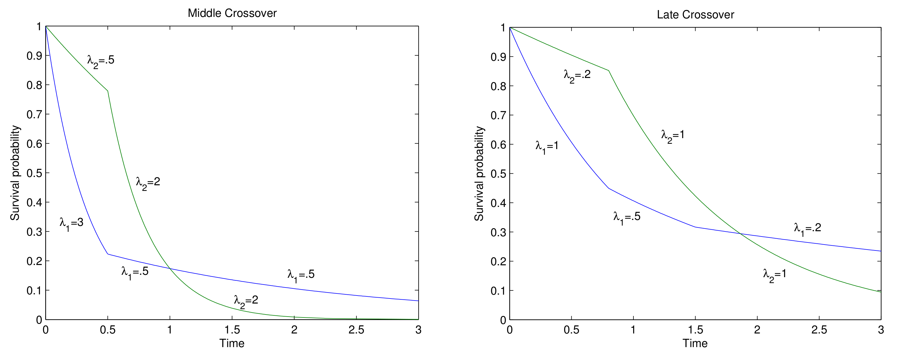
Simulations on power were also conducted under some specific alternatives, in order to check the performance of the tests associated with the weight functions. For this, we considered the three settings in which the AFT model does not hold: (S1) the model of [20], which accommodates crossing hazard functions with β 1 and β 2 taken with opposite signs (see [20] for details); (S2) survival curves cross near the middle of the time course; (S3) late crossing of survival curves appears. For the cases of S2 and S3, we generated data from piecewise exponential distributions that have constants λ i for group i, i = 1 , 2 , and the censoring distributions were c × U n i f o r m ( 0 , 1 ) , with c chosen to produce specified censoring proportions. For example, the c values of 3.2, 1.5, and 0.75 led to the censoring proportions of 20%, 40%, and 60%, respectively, in S2 (middle crossover). For the middle survival differences λ 1 = 3, 0.5, 0.5 and λ 2 = 0.5, 2, 2 for t < 0.5 , 0.5 t < 0.6 , t 0.6 , respectively. For the late survival differences, λ 1 = 1, 0.5, 0.2 and λ 2 = 0.2, 1, 1 for t < 0.8 , 0.8 t < 1.5 , t 1.5 , respectively. Figure 2 provides visual illustrations of the cases of S2 and S3. Simulation results of these three cases are presented in Table 3. The results of S1–S3 demonstrate that the improvements of the G ρ family by using the weight function W n * were notable overall, outperforming the log-rank. It becomes more apparent that the tests with W n * improved upon the others, as sample size and censoring proportion, respectively, became smaller and heavier. For example, for the small sample of n 1 = n 2 = 25 in the case of S2, powers with G 1 , G 2 , W 1 * , and W 2 * were 15.8%, 21.2%, 16.5%, and 22.1%, respectively. This indicates that the performances of the G ρ family by using the weight function W n * when light censoring (20%) were improved by 4% (15.8% to 16.5% for ρ = 1 ) and 4% (21.2% to 22.1% for ρ = 2 ). For moderate censoring (40%), they increased up to 10% (20.5% to 22.6% for ρ = 1 ) and 9% (23.8% to 26% for ρ = 2 ). When the censoring proportion was heavy (60%), the performance made a more than 20% increase. Specifically, the performance improved by 24%, making a move from 18.9% to 23.4%, for ρ = 1, and 72% (21.7% to 37.5%) for ρ = 2. Similar phenomena were observed in other settings including the case S3. It is worth noting that from Table 3, it can be seen that as the percentage of censoring increased, the power increased, which is a reversal phenomenon. In general, with higher censoring, one would expect less power. However, the reversal phenomenon in the right censoring case would be feasible. This is because early survival differences were mainly observed as the censoring proportion increases. For example, little or no power is possible by the crossover in the survival functions even when light or no censoring occurs. Note that all simulations were performed using MATLABm in which the methods were implemented. Source code is available upon reasonable request.

3.2. Application

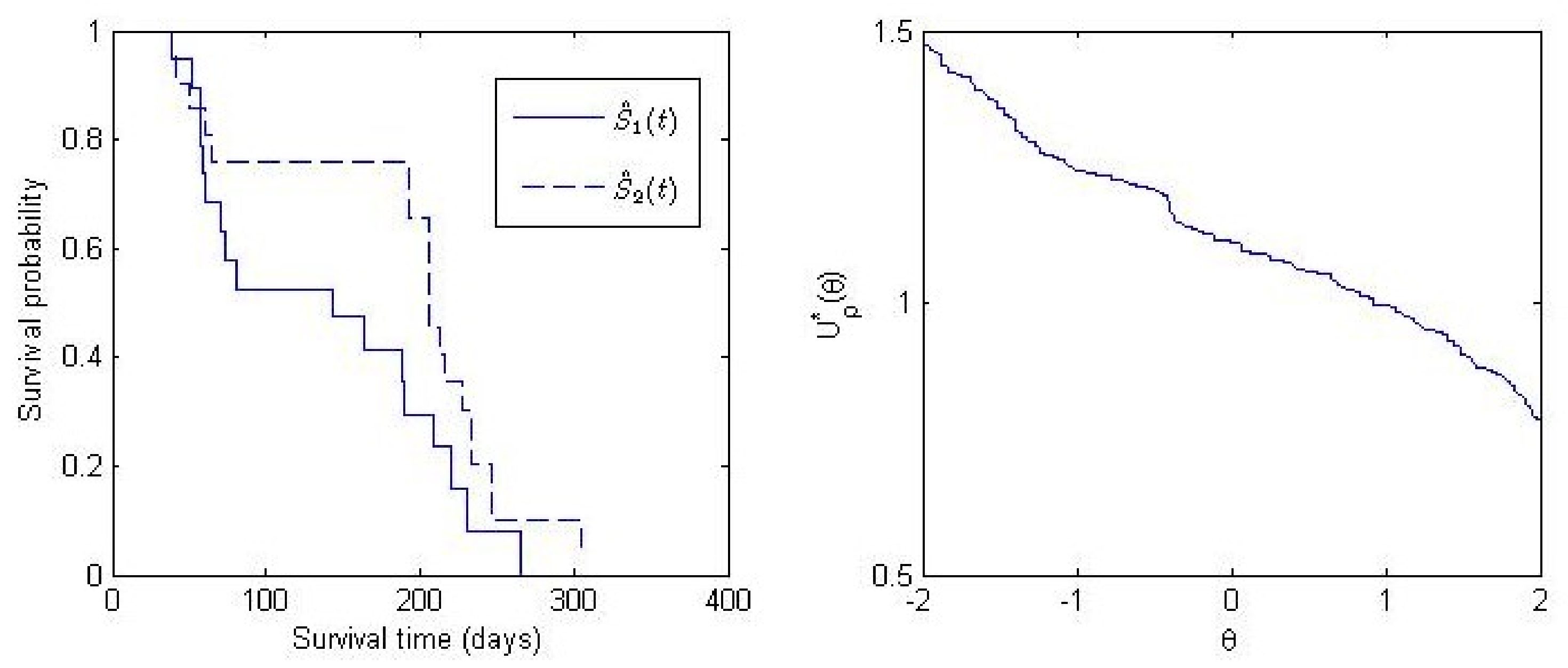
The procedures evaluated in the simulation study were applied to real world data concerning vaginal cancer, which is a disease in which malignant cells grow abnormally in the vagina. It was reported in the study of human disease that vaginal cancer is predominantly a disease of older women, and approximately 50% of cases are present in women over the age of 70 ([21]). In this work, data on vaginal cancer in female rats ([22]) was used, where rats with the disease were split up into two groups by pretreatment regimen with samples of sizes n 1 = 19 and n 2 = 21. Two censored datasets were observed in each group. Times to cancer mortality from vaginal cancer or censoring following treatment of rats insulted with carcinogen DMBA were the variables of interest. Note that it was found that the two-sample scale model described the effect of the pretreatment regime well ([3,23]). The plot on the left in Figure 3 displays the two estimated survival functions of the two groups.
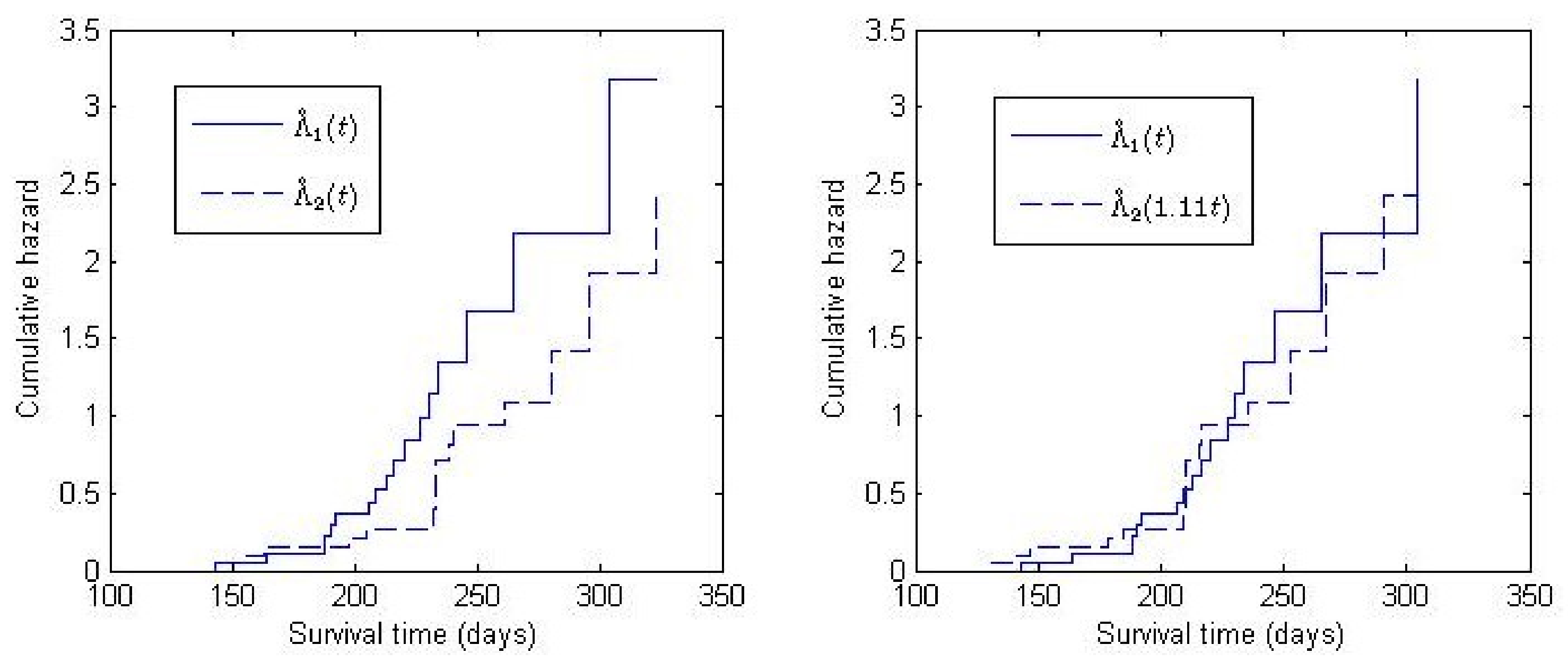
Table 4 summarizes point estimates, empirical p-values, and confidence intervals for the scale parameter with the weight functions being considered. Results show that the vaginal cancer data can be reasonably fit by a two-sample scale model, Λ 1 ( t ) = Λ 2 ( θ t ) , thus confirming the previous works ([3,23]). The weighted log-rank statistics in the table yields θ ^ 1.1 , which implies a 10% difference approximately in effectiveness between the pretreatment regimen on the survival. It is questionable whether the improvement on the survival by 10% is significant. The plot on the right in Figure 3 is a plot of U ρ * ( θ ) versus θ , illustrating how to obtain the estimated value of θ . The estimated cumulative hazard curves of the two groups are compared in Figure 4. The figure (left) depicts the estimated curves of the two groups, providing an initial insight into the shape of the curves. The figure (right) presents the same with the time scale adjusted between the cumulative hazard functions; the two curves have approximately the same shape, which reveals the suitability of the two-sample AFT model.

4. Concluding Remarks

The sensitivity of inference procedures of the G ρ family of weighted log-rank tests varies depending on the choice of weight functions. It may lose power when two hazard functions cross. For example, in a clinical study comparing two treatments offering different benefits over time, one treatment could be effective immediately, whereas the other may have long-term effects. Thus, carefully chosen weight functions should be used in applications. This work modified the G ρ family of weighted log-rank tests so that it can be used for the AFT model, improving its performance in realistic situations. The procedures are based on the weight function that has a censoring proportion as a factor in it. Simulation results demonstrated that the modified weight function makes the G ρ family more dependable in realistic alternatives, dealing with heavy censoring. The weight function in this work, with some modifications, could also be used to handle rare events’ data for the AFT model. In addition, the weight function could be further extended to a censored regression with covariates. Finally, to deal with the situation of crossing hazard, some versatile tests based on the simultaneous use of the weighted log-rank statistics associated with the weight function, such as Rényi-type tests (Gill, 1980), could be utilized, rather than using locally powerful tests.

Funding

This research received no external funding.

Institutional Review Board Statement

Not applicable.

Informed Consent Statement

Not applicable.

Conflicts of Interest

The author declares no conflict of interest.

References

  1. Louis, T.A. Non-parametric analysis of an accelerated failure time model. Biometrika 1981, 68, 381–390. [Google Scholar] [CrossRef]
  2. Prentice, R.L. Linear rank tests with right censored data. Biometrika 1978, 65, 167–179. [Google Scholar] [CrossRef]
  3. Wei, L.J.; Gail, M.H. Nonparametric estimation for a scale-change with censored observations. J. Am. Stat. Assoc. 1983, 78, 312–318. [Google Scholar] [CrossRef]
  4. Fleming, T.R.; Harrington, D.P. A Class of Hypothesis Tests for One and Two Samples of Censored Survival Data. Commun. Stat. Theory Methods 1981, 13, 2469–2486. [Google Scholar] [CrossRef]
  5. Fleming, T.R.; Harrington, D.P.; O’Sullivan, M. Supremum versions of the Log-Rank and Generalized Wilcoxon Statistics. J. Am. Stat. Assoc. 1987, 82, 312–320. [Google Scholar] [CrossRef]
  6. Harrington, D.P.; Fleming, T.R. A class of rank test procedures for censored survival data. Biometrika 1982, 69, 133–143. [Google Scholar] [CrossRef]
  7. Kaplan, E.; Meier, P. Nonparametric Estimation from Incomplete Observations. J. Am. Assoc. 1958, 53, 457–481. [Google Scholar] [CrossRef]
  8. Buyske, S.; Fagerstrom, R.; Ying, Z. A class of weighted log-rank tests for survival data when the event is rare. J. Am. Stat. Assoc. 2000, 95, 249–258. [Google Scholar] [CrossRef]
  9. Lee, S.H.; Lee, E.J. On testing equality of two censored samples. J. Stat. Comput. Simul. 2009, 81, 1017–1026. [Google Scholar] [CrossRef]
  10. Shen, Y.; Cai, J. Maximum of the Weighted Kaplan–Meier Tests with Applications to Cancer Prevention and Screening Trials. Biometrics 2001, 57, 837–843. [Google Scholar] [CrossRef]
  11. Wu, L.; Gilbert, P.B. Flexible Weighted Log-Rank Tests Optimal for Detecting Early and/or Late Survival Differences. Biometrics 2002, 58, 997–1004. [Google Scholar] [CrossRef]
  12. Aalen, D.D. Nonparametric inference for a family of counting processes. Ann. Stat. 1978, 6, 701–726. [Google Scholar] [CrossRef]
  13. Nelson, W. Hazard plotting for incomplete failure data. J. Qual. Technol. 1969, 1, 27–52. [Google Scholar] [CrossRef]
  14. Hodges, J.L.; Lehmann, E.L. Estimation of location based on ranks. Ann. Math. Stat. 1963, 34, 598–611. [Google Scholar] [CrossRef]
  15. Gill, R.D. Censoring and Stochastic Integrals; MC Tract 124; Mathematical Centre: Amsterdam, The Netherlands, 1980. [Google Scholar]
  16. Cox, D.R. Regression models and life tables (with discussion). J. R. Stat. Soc. 1972, 34, 187–220. [Google Scholar]
  17. Mantel, N. Evaluation of Survival Data and Two New Rank Order Statistics Arising in Its Consideration. Cancer Chemother. Rep. 1966, 50, 163–170. [Google Scholar]
  18. Peto, R.; Peto, J. Asymptotically efficient rank invariant test procedures (with discussion). J. R. Stat. Soc. Ser. A 1972, 135, 185–207. [Google Scholar] [CrossRef]
  19. Lee, S.H.; Yang, S. Checking the censored two-sample accelerated life model using integrated cumulative hazard difference. Lifetime Data Anal. 2007, 13, 371–380. [Google Scholar] [CrossRef]
  20. Yang, S.; Prentice, R. Semiparametric analysis of short-term and long-term and hazard ratios with two-sample survival data. Biometrika 2005, 92, 1–17. [Google Scholar] [CrossRef]
  21. Creasman, W.T.; Phillips, J.L.; Menck, H.R. The National Cancer Data Base report on cancer of the vagina. Cancer 1998, 83, 1033–1040. [Google Scholar] [CrossRef]
  22. Pike, M.C. A method of analysis of a certain class of experiments in carcinogensis. Biometrika 1966, 18, 303–328. [Google Scholar]
  23. Kalbfleisch, J.D.; Prentice, R.L. The Statistical Analysis of Failure Time Data; Wiley: New York, NY, USA, 1980. [Google Scholar]
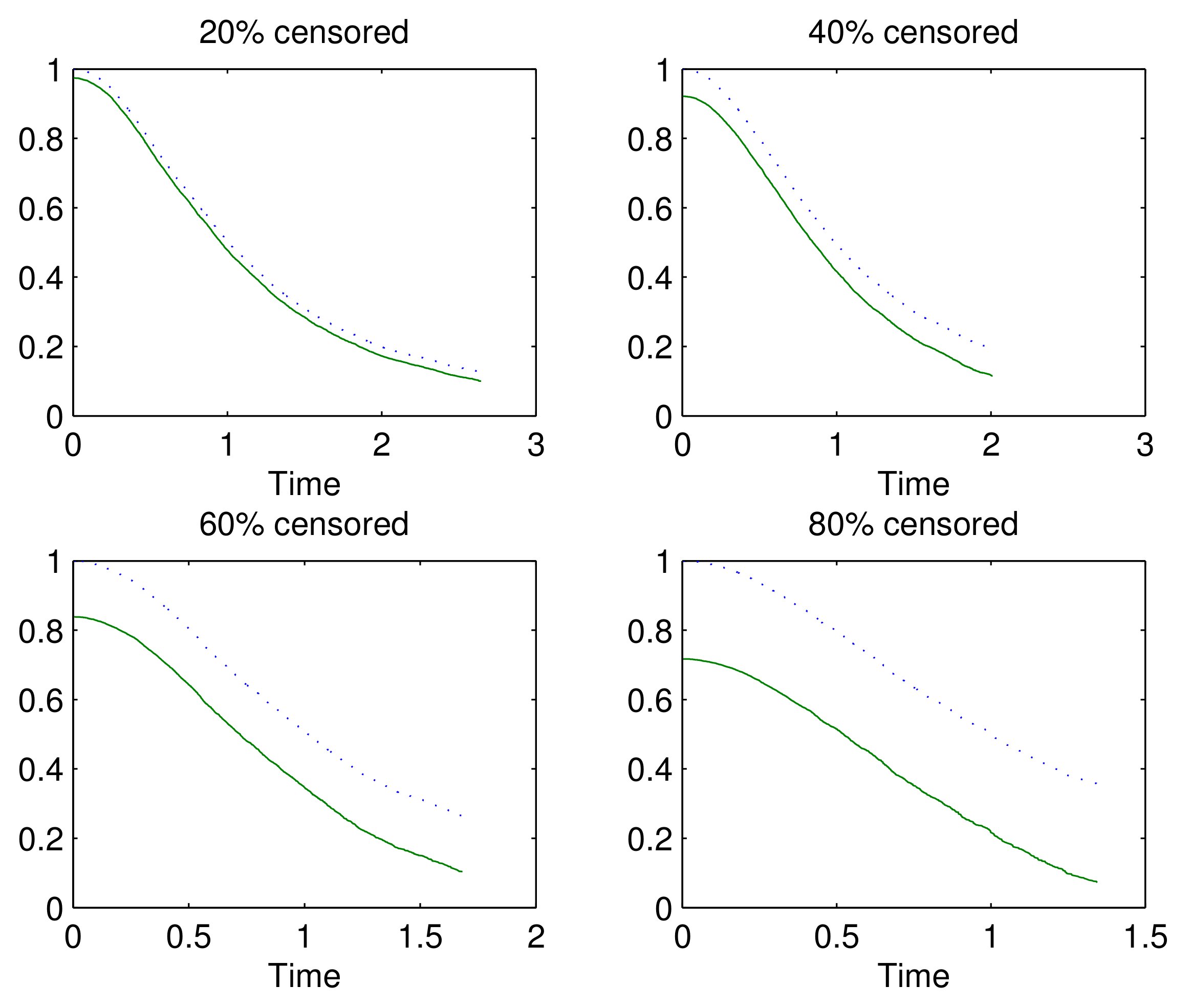
Figure 1. Weight comparison, W ( t ) (dotted) and W n * ( t ) (solid) with ρ = 1 .
Stats 04 00023 g001
Figure 2. Configurations for crossing survival curves.
Stats 04 00023 g002
Figure 3. Estimated survival functions (left) and U ρ * with ρ = 1 (right), vaginal cancer.
Stats 04 00023 g003
Figure 4. Estimated cumulative hazard functions, vaginal cancer.
Stats 04 00023 g004
Table 1. Empirical coverage probability (ECP, %) and empirical mean length (EML) of confidence interval at α = 0.05 , θ = 2 .
( n 1 , n 2 ) Censoring % G 1 G 2 W 1 * W 2 * Log-Rank
C1
(25, 25)2094.8 (2.0616) 95.5 (2.1151)94.9 (2.0620)95.5 (2.1205)94.5 (2.1326)
4095.2 (2.1329)94.7 (2.1851)95.3 (2.1380)94.8 (2.2025)93.8 (2.1557)
6095.9 (2.3495)95.9 (2.3825)96.2 (2.3586)96.1 (2.4074)95.8 (2.3583)
(25, 50)2094.6 (1.8030)94.6 (1.8568)94.6 (1.8038)94.7 (1.8629)94.6 (1.9095)
4095.2 (1.9196)96.1 (1.9778)95.2 (1.9234)96.5 (1.9910)94.2 (1.9641)
6095.0 (2.1359)94.7 (2.1710)95.1 (2.1442)94.8 (2.1974)94.6 (2.1568)
(50, 50)2095.9 (1.4851)95.4 (1.5312)95.8 (1.4858)95.5 (1.5365)95.5 (1.5861)
4093.9 (1.6014)95.0 (1.6459)94.1 (1.6045)95.0 (1.6607)94.0 (1.6591)
6096.6 (1.8615)96.2 (1.8991)96.2 (1.8700)96.0 (1.9245)95.5 (1.8859)
C2
(25, 25)2096.3 (1.5116)95.4 (1.6989)96.3 (1.5183)95.4 (1.7093)94.9 (1.3485)
4094.2 (1.7866)95.4 (1.9407)94.3 (1.8003)95.5 (1.9607)94.3 (1.6406)
6094.8 (2.0684)94.4 (2.1258)94.7 (2.0901)94.5 (2.1978)94.4 (1.9845)
(25, 50)2094.4 (1.3042)94.5 (1.4993)94.5 (1.3111)94.7 (1.5095)94.3 (1.1393)
4093.8 (1.4782)94.0 (1.6497)93.7 (1.4931)94.1 (1.6734)93.0 (1.3364)
6094.9 (1.7854)94.6 (1.9165)94.7 (1.8073)94.7 (1.9526)94.7 (1.6711)
(50, 50)2094.3 (1.0434)94.6 (1.1927)94.3 (1.0484)94.5 (1.2000)93.9 (0.9226)
4095.3 (1.2081)94.6 (1.3440)95.3 (1.2204)94.6 (1.3621)95.2 (1.1028)
6094.5 (1.5267)94.7 (1.6326)94.6 (1.5465)94.5 (1.6551)94.9 (1.4419)
C3
(25, 25)2094.8 (2.2620)94.7 (2.2907)94.7 (2.2621)94.5 (2.2974)94.9 (2.3131)
4094.9 (2.3852)95.2 (2.3995)95.0 (2.3876)95.4 (2.4144)94.9 (2.4076)
6094.6 (2.4918)94.9 (2.4981)94.5 (2.4944)95.2 (2.5185)94.5 (2.5072)
(25, 50)2094.7 (2.0501)94.5 (2.0954)94.6 (2.0520)94.9 (2.1034)95.0 (2.0993)
4096.3 (2.1733)96.0 (2.1848)96.1 (2.1747)96.0 (2.1971)96.5 (2.2082)
6095.6 (2.3492)95.7 (2.3517)95.5 (2.3486)95.6 (2.3662)95.4 (2.3694)
(50, 50)2095.2 (1.7322)95.7 (1.7552)95.3 (1.7321)95.7 (1.7613)94.9 (1.8090)
4095.3 (1.8365)95.4 (1.8388)95.2 (1.8356)95.7 (1.8496)95.5 (1.8846)
6095.0 (2.0581)95.0 (2.0573)95.4 (2.0575)95.0 (2.0693)94.8 (2.0763)
: ECP (EML); W 1 * = W n * with p = 1 , W 2 * = W n * with p = 2 .
Table 2. Size simulation results (%) at α = 0.05 , θ = 2 .
( n 1 , n 2 ) Censoring % G 1 G 2 W 1 * W 2 * Log-Rank
C1
(25, 25)206.26.96.17.07.4
409.19.59.29.58.5
609.910.09.910.59.7
(25, 50)206.87.36.67.37.5
407.87.87.27.97.4
609.29.29.49.99.3
(50, 50)204.44.94.45.05.9
406.77.46.87.56.6
609.39.79.86.69.1
C2
(25, 25)203.85.44.05.42.7
404.66.15.06.54.2
608.19.58.89.87.1
(25, 50)204.15.04.15.13.0
403.85.54.25.73.9
606.57.56.67.65.8
(50, 50)202.23.32.23.51.9
403.44.13.54.52.4
606.25.75.36.85.9
C3
(25, 25)208.18.17.98.57.6
408.29.58.79.86.9
607.88.189.56.6
(25, 50)207.57.87.97.97.0
408.08.58.29.06.7
607.57.98.29.57.1
(50, 50)206.57.56.58.06.0
406.67.37.08.16.5
607.27.87.58.26.8
W 1 * = W n * with p = 1 , W 2 * = W n * with p = 2 .
Table 3. Power simulation results (%).
( n 1 , n 2 ) Censoring % G 1 G 2 W 1 * W 2 * Log-Rank
S1
(25, 25)2015.821.216.522.110.3
4020.523.822.626.216.2
6018.921.723.227.518.1
(25, 50)2017.623.119.624.011.2
4020.323.722.927.016.2
6025.127.430.032.421.5
(50, 50)2014.922.919.623.78.1
4022.028.125.030.216.1
6026.128.929.132.224.0
S2
(25, 25)2046.567.048.768.711.5
4057.069.159.972.132.0
6070.874.974.576.860.8
(25, 50)2051.072.752.373.914.2
4063.277.667.181.232.5
6077.481.680.683.267.3
(50, 50)2060.885.263.587.010.4
4071.686.876.689.535.0
6088.290.290.291.581.6
S3
(25, 25)208.426.29.228.41.2
4020.830.822.636.08.0
6031.239.436.848.622.6
(25, 50)2011.028.411.629.60.8
4018.635.221.240.25.2
6035.244.441.657.423.6
(50, 50)207.427.28.628.80.1
4014.834.020.441.01.8
6042.053.050.266.228.4
W 1 * = W n * with p = 1 , W 2 * = W n * with p = 2 .
Table 4. Point estimates and p–values, vaginal cancer.
G 1 G 2 W 1 * W 2 * Log-Rank
p-value0.490.480.490.480.49
θ ^ 1.111.101.111.101.13
95% C.I.(0.99, 1.25)(0.96, 1.24)(0.99, 1.25)(0.96, 1.24)(0.98, 1.30)
Publisher’s Note: MDPI stays neutral with regard to jurisdictional claims in published maps and institutional affiliations.