Kolmogorov-Arnold Networks for Interpretable Analysis of Water Quality Time-Series Data

Abstract

Kolmogorov–Arnold networks (KANs) represent a promising modeling framework for applications requiring interpretability. In this study, we investigate the use of KANs to analyze time series of water quality parameters obtained from a publicly available dataset related to an aquaponic environment. Two water quality indices (WQIs) were computed—a linear case based on the weighted average WQI, and a non-linear case using the weighted quadratic mean (WQM) WQI, both derived from three water parameters: pH, total dissolved solids (TDS), and temperature. For each case, KAN models were trained to predict the respective WQI, yielding explicit algebraic expressions with low prediction errors and clear input–output mathematical relationships. Model performance was evaluated using standard regression metrics, with $R^2$ values exceeding 0.96 on the hold-out test set across all cases. Specifically for the non-linear WQM case, we trained 15 classical regressors using the LazyPredict Python library. The top three models were selected based on validation performance. They were then compared against the KAN model and its symbolic expressions using a 5-fold cross-validation protocol on a temporally shifted test set (approximately one month after the training period), without retraining. Results show that KAN slightly outperforms the best tested baseline regressor (multilayer perceptron, MLP), with average $R^2$ scores of $0.998\pm 0.001$ and $0.996\pm 0.001$, respectively. These findings highlight the potential of KAN in terms of predictive performance, comparable to well-established algorithms. Moreover, the ability of KAN to extract data-driven, interpretable, and lightweight symbolic models makes it a valuable tool for applications where accuracy, transparency, and model simplification are critical.

1. Introduction

Kolmogorov–Arnold networks (KANs) are a promising artificial neural network (ANN) architecture recently proposed as a novel paradigm [1,2]. KAN models possess valuable properties that enhance both accuracy and interpretability compared to traditional ANN approaches [3,4]. Notably, KANs offer inherent interpretability by enabling the derivation of closed-form mathematical expressions that describe input–output relationships, a property associated with symbolic regression [5].

In this work, we train KAN models to analyze time-series data collected from an internet of things (IoT)-based water quality monitoring system in an aquaponic environment [6]. The main objective is to evaluate the capacity of KAN to extract symbolic expressions that accurately model the relationship between input water parameters and the water quality index (WQI), a composite indicator derived from normalized measurements of pH, total dissolved solids (TDS), and temperature. Two WQI formulations are addressed as separate case studies: the weighted arithmetic WQI (WA-WQI) and the weighted quadratic mean WQI (WQM-WQI). Although numerous WQI formulations exist in the literature [7,8], our aim is not to compare index designs, but to use WQI as a practical application context for testing KAN’s modeling and interpretability capabilities.

The trained KAN models achieved satisfactory predictive performance for both WQI formulations, as measured by standard regression metrics: mean absolute error (MAE), root mean squared error (RMSE), and the coefficient of determination (R²) [9]. In each case, symbolic expressions derived from the models preserved prediction accuracy while yielding compact and interpretable approximations. The trained KAN models and their symbolic forms were also benchmarked against several baseline regressors, including multilayer perceptrons, tree-based models, and ensemble methods, demonstrating KAN’s competitiveness in terms of both performance and interpretability. Notably, symbolic expressions extracted from pruned KAN models reduced the number of input variables while maintaining high predictive accuracy, underscoring their value for model simplification and feature selection.

The findings from both case studies support the use of KAN in applications where transparency and accuracy are important. In addition to producing interpretable symbolic functions, KAN demonstrated feature selection capabilities via sparsification, further supported by statistical feature relevance analysis.

The remainder of this paper is organized as follows. Section 2 details the dataset, preprocessing steps, WQI computation, a brief overview of the KAN theoretical foundations, implementation details, and the data splitting strategies used for training, validation, and testing. Section 3 presents and discusses the main results, including model pruning, symbolic expression extraction, and comparisons with baseline regressors. Finally, Section 4 summarizes the main findings and outlines directions for future work.

2. Material and Methods

2.1. Dataset Description

The dataset used in this study consists of water quality measurements collected from an aquaponic fish pond monitored with IoT sensors [6]. The monitored variables and their corresponding units are summarized in

Table 1. Water quality variables and their units as measured by IoT sensors.

Description	Units
Timestamp recorded	Date Time
Water pH	pH units
TDS concentration	mg/L (ppm)
Water temperature	°C (Celsius)

.

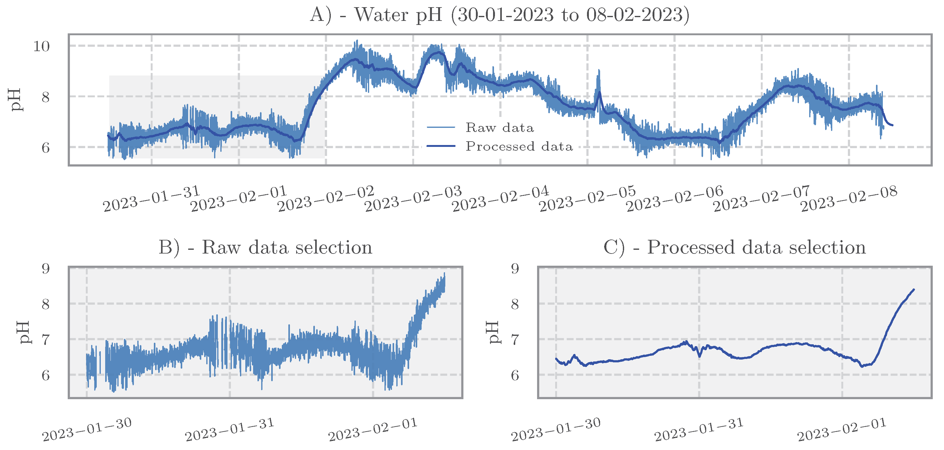
Data Cleaning and Preprocessing

IoT sensor networks, while enabling large-scale and continuous environmental monitoring, are prone to various data quality challenges [10]. Common issues include sensor malfunctions, power instability, intermittent connectivity, and communication failures. These problems often manifest as missing values, irregular sampling intervals, or noisy measurements. To address these challenges and ensure data reliability, appropriate cleaning and preprocessing steps are essential prior to any modeling or analysis [11,12].

In this study, the original dataset was not uniformly sampled, necessitating preprocessing to obtain a consistent time series structure. For model training, validation, and testing under a classical hold-out cross-validation scheme [13], we selected data from 30 January to 8 February 2023, representing nine consecutive days. Additionally, a separate segment spanning 3.5 days—from 4 March to 7 March 2023—was used exclusively for a more rigorous 5-fold cross-validation procedure [14]. Details of these data splits are provided in Section 2.5.

We applied a mean aggregation procedure to resample the data at a 1-min interval to achieve uniform temporal resolution. Despite this aggregation, some missing values remained due to irregularities in the original recordings. These gaps were addressed using linear interpolation, which estimates the missing values by fitting a local linear curve to neighboring points.

Finally, to reduce sensor-induced noise and smooth short-term fluctuations, we applied a single-pole recursive infinite impulse response (IIR) filter to each time series [15]. This step produced continuous, smoothed signals while preserving the broader trends relevant to subsequent modeling. The resulting preprocessed dataset is uniformly sampled, free of missing values, and smoothed, forming a consistent input for developing, training, and evaluating the models described in the following sections.

2.2. WA-WQI and WQM-WQI Case Study Formulations

The water quality index (WQI) is a widely used metric for assessing water quality [7,8]. Typically, such indices are calculated by mathematically combining measurements of water parameters. The calculation process generally involves the following steps: (1) variable selection, (2) parameter scaling, (3) weighting, and (4) algebraic aggregation [8,16]. Experts can assess water quality in specific contexts based on the computed index.

This work presents two case studies, each defined by a distinct WQI aggregation function adopted as the prediction target. The first is the weighted arithmetic WQI (WA-WQI), and the second is the weighted quadratic mean WQI (WQM-WQI) [8,16]. These formulations were chosen not only for their conceptual simplicity and interpretability but also to allow comparative analysis under linear and nonlinear aggregation structures. The WA-WQI was selected for the initial case study, serving as a benchmark due to its wide adoption and transparent computation. Its formulation is shown in Equation (1), where i indexes the input variables (pH, TDS, and temperature), and $N=3$ denotes the total number of variables.

$$\mathrm{WA}-\mathrm{WQI}={\displaystyle \frac{{\sum }_{i=1}^N{w}_i{Q}_i}{{\sum }_{i=1}^N{w}_i}}$$

(1)

where:

• $Q_i$ is the sub-index quality rating (scaled between 0 and 100),
• $w_i$ is the weight assigned to each variable.

The second aggregation function, WQM-WQI, is a weighted root mean square (quadratic mean) of the sub-index ratings. Its expression is shown in Equation (2), using the same variables and weights defined above.

$$\mathrm{WQM}-\mathrm{WQI}=\sqrt{\sum _{i=1}^N{w}_i{Q}_i^2}$$

(2)

Since the dataset includes three key variables (water pH, TDS, and water temperature), each is mapped to a quality rating $Q_i$ according to its specific characteristics, as described below.

2.2.1. Quality Rating Calculation

The quality rating for each variable was transformed using scaling functions that aimed to map the values to a range close to 0–100, representing conditions from poor to ideal water quality. These transformations were based on the observed value ranges from the dataset used in this study [6] and guided by similar normalization approaches reported in the literature [17]. While the specific equations were heuristically designed, they reflect practical scaling practices. Importantly, due to the data-driven learning capabilities of KAN models, the method is expected to remain robust to changes in parameter transformations or rating scales [5,18], further supporting its applicability across different water quality assessment schemes.

pH Quality Rating ($Q_{\mathrm{pH}}$), Equation (3)

$$Q_{\mathrm{pH}}=\left({\displaystyle \frac{V_{\mathrm{pH}}-7}{8.5-7}}\right)\times 100$$

(3)

where:

• $V_{\mathrm{pH}}$ = observed pH value
• Ideal pH = 7.0 (neutral)
• Standard maximum = 8.5

Inverse Scaled TDS Quality Rating ($Q_{\mathrm{TDS}}$), Equation (4)

$$Q_{\mathrm{TDS}}={\displaystyle \frac{500-V_{\mathrm{TDS}}}{500}}\times 100$$

(4)

where:

• $V_{\mathrm{TDS}}$ = observed TDS value
• Ideal TDS = 0 mg/L
• Standard maximum = 500 mg/L
• Higher TDS indicates worse quality (inverse scaling)

Temperature Quality Rating ($Q_{\mathrm{Temp}}$), Equation (5)

$$Q_{\mathrm{Temp}}=\left(1-{\displaystyle \frac{|V_{\mathrm{Temp}}-26|}{3}}\right)\times 100$$

(5)

where:

• $V_{\mathrm{Temp}}$ = observed water temperature
• Ideal temperature = 26 °C
• Acceptable range = 24–27 °C
• Deviation from 26 °C results in a penalty

2.2.2. Weight Calculation

The weight for each variable is calculated as inversely proportional to its maximum permissible value, Equation (6):

$$w_i={\displaystyle \frac{k}{S_i}}$$

(6)

where:

• $S_i$ = standard limit for each variable
• k = proportionality constant (set to 1 for simplicity)

For this study, we used the following limits:

• $S_{\mathrm{pH}}=8.5$
• $S_{\mathrm{TDS}}=500$
• $S_{\mathrm{Temp}}=3$ (deviation range from 26 °C)

By combining the quality ratings and weights according to Equations (1) and (2), the final WQI values are computed, providing composite assessments of water quality based on the selected parameters. While the specific quality rating functions and thresholds used in this study were tailored to the presented case studies, alternative normalization schemes or WQI formulations could be employed to suit different applications. Such adjustments would not alter the core objectives of this study, which focus on evaluating the capabilities of KAN in modeling interpretable relationships from real-world water quality data.

2.3. Kolmogorov–Arnold Networks: Theoretical Foundations

Multilayer Perceptron (MLP) networks are based on the foundational principle that multilayer feedforward networks are universal approximators of any continuous function [19,20]. In contrast, Kolmogorov–Arnold Networks (KAN) are based on the Kolmogorov–Arnold superposition theorem (K–A theorem) [21,22].

The K–A theorem states that any multivariate continuous function $f\left(\mathbf{x}\right)$, in which $\mathbf{x}=\{x_1,x_2,\dots ,x_n\}$, defined on a bounded domain, can be expressed as a combination of a finite number of continuous univariate functions. This formulation is mathematically described in Equation (7).

$$f\left(\mathbf{x}\right)=\sum _{q=0}^{2n}{\Phi }_q\left(\sum _{p=1}^n{\varphi }_{pq}\left(x_p\right)\right)$$

(7)

where:

• $f\left(\mathbf{x}\right)$—the target multivariate function to approximate.
• $x_p$—the p-th input variable.
• ${\varphi }_{pq}$—continuous univariate inner functions, applied to each input variable.
• ${\Phi }_q$—continuous univariate outer functions, combining the intermediate results.
• n—the dimensionality of the input space.

In practice, KAN implements this theoretical formulation by constructing a network where the inner functions (${\varphi }_{pq}$) and outer functions (${\Phi }_q$) are approximated using neural network layers. This structure enables KAN to efficiently model complex relationships while retaining interpretability through the explicit mathematical expressions derived from the network’s learned functions.

For the sake of simplicity, we recommend that interested readers consult [1,2] for a more in-depth theoretical background and implementation details.

2.4. KAN Implementation Details

The univariate functions ${\varphi }_{pq}$ and ${\Phi }_q$ in Equation (7) are implemented in KAN as smooth, learnable functions constructed using a linear combination of basis functions known as B-splines [23]. B-splines are a specific class of spline functions that offer desirable properties such as local support, smoothness, and differentiability, making them particularly suitable for neural network training via backpropagation [24,25]. In practice, a univariate function $\varphi \left(x\right)$ within a KAN is represented as in Equation (8):

$$\varphi \left(x\right)=\sum _{i=0}^{G+k-1}{c}_i{B}_i\left(x\right)$$

(8)

where $B_i\left(x\right)$ is the i-th B-spline basis function of degree k, $c_i$ are learnable coefficients, and G is the number of grid intervals (also referred to as segments or knots) that define the piecewise structure.

In this study, we adopted a commonly used configuration of cubic B-splines ($k=3$) and selected $G=7$ intervals to balance model flexibility and computational efficiency, consistent with prior KAN implementations [1].

To represent the layered structure of a KAN, each layer is defined as a matrix ${\Phi }^l$ whose entries are univariate functions ${\varphi }_{ij}$ mapping from input neuron i to output neuron j. Unlike traditional neural networks, where weights are scalar values, the connections in KAN are functional—each entry in the matrix is a spline-based function learned during training.

A KAN layer l is thus denoted as:

$${\Phi }^l:[N_{in}^l,N_{out}^l]$$

where $N_{in}^l$ and $N_{out}^l$ refer to the number of input and output units, respectively. Given an input vector $\mathbf{x}$, the operation of two consecutive KAN layers is expressed as in Equation (9):

$$y=\mathrm{KAN}\left(\mathbf{x}\right)=\left({\Phi }^2\circ {\Phi }^1\right)\left(\mathbf{x}\right)$$

(9)

where ∘ denotes function composition, not matrix multiplication. Each layer applies a learned set of univariate transformations to its inputs, sums them at the node level, and passes them to the next layer.

Motivation and Feasibility of Model Pruning

KAN models offer the advantage of producing interpretable symbolic expressions by learning univariate functions. When combined according to the formulation in Equation (7), these functions capture the input–output relationship in a structured and mathematically transparent manner. However, as with traditional neural networks, not all input features, network nodes, or connections contribute equally to the final prediction. Reducing unnecessary components within the network—without significantly degrading performance—is desirable to enhance interpretability and deployment efficiency [1,2]. By definition, pruned KAN models are expected to be considerably more interpretable than their non-pruned counterparts.

A common practical strategy involves starting with a more complex architecture and subsequently applying sparsification and pruning techniques to obtain a compact model [1]. This process aims to maximize interpretability while maintaining performance. In this context, we evaluated the feasibility of a feature pruning strategy with two main motivations: (i) to identify and eliminate inputs that contribute minimally to the learned function, and (ii) to simplify the resulting symbolic expression, thereby improving transparency and interpretability.

Given the data-driven nature of KAN models and their ability to represent functional dependencies explicitly, pruning non-informative components is both feasible and advantageous. As demonstrated in the following sections, our pruning strategy produced a reduced model that retained high predictive accuracy while yielding a more compact symbolic representation. This confirms the practical utility of pruning in real-world scenarios, particularly where interpretability and model parsimony are essential.

Following this rationale, we implemented two distinct KAN model architectures and applied both to each of the two case studies: the linear WA-WQI and the nonlinear WQM-WQI. The original model incorporates all three input variables and has a more complex internal structure with additional hidden units. The pruned model, obtained via feature sparsification, uses only two inputs (pH and temperature) and adopts a more compact architecture with fewer internal nodes. The configurations of both models are as follows:

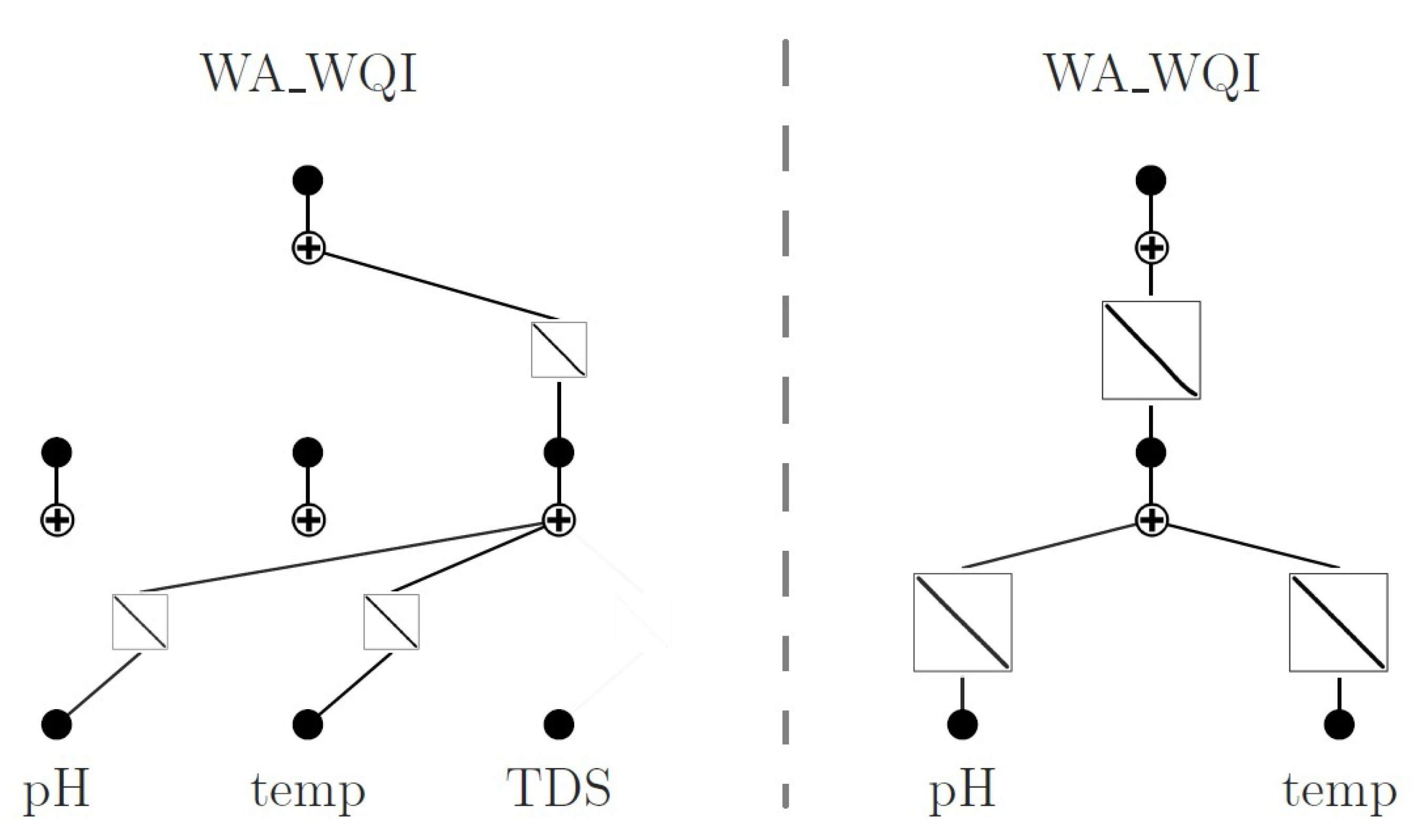
• Original model (KAN): Two layers configured as ${\Phi }^1:[3,3]$, ${\Phi }^2:[3,1]$, using all three input variables (pH, TDS, temperature).
• Pruned model (KAN′): Two layers configured as ${\Phi }^1:[2,1]$, ${\Phi }^2:[1,1]$, using only pH and temperature after feature sparsification.

As previously described, both models were trained to predict the WQI using their respective input configurations, and were applied to both WA-WQI and WQM-WQI formulations. Further details on this pruning strategy and its implications are provided in Section 3. Symbolic expressions were extracted from the learned univariate B-spline-based functions for each trained model. These expressions allow WQI predictions to be made without executing the whole network, showcasing a key strength of KAN: its ability to produce interpretable, compact mathematical representations of the modeled relationships. We computed $R^2$, MAE, and RMSE metrics for both models and their corresponding symbolic expressions to evaluate performance.

2.5. Data Split and Evaluation Protocols

To ensure a reliable assessment of model performance, we adopted two complementary validation strategies tailored to the two case studies presented in this work. For the first case study, which focuses on predicting the WA-WQI, we employed a classical hold-out validation scheme. The dataset was split into training, validation, and test subsets, following standard practices in ML workflows. For the second case study, focused on predicting the WQM-WQI, we also applied a hold-out split to define the training, validation, and test subsets. However, the main difference lies in the use of the test subset, which served as the basis for an additional 5-fold temporal cross-validation. This protocol was designed to more rigorously assess model generalization under temporally realistic conditions. The test subset used for temporal validation was collected approximately one month after the training period and spans 3.5 consecutive days. Each fold consists of a 2-day segment, shifted forward by 8-h steps, simulating a sliding-window scenario. The partitioning strategies and corresponding evaluation protocols for each case study are detailed in the following subsections.

2.5.1. Hold-Out Cross-Validation: Study Case 1

A selected data window spanning from 2023-01-30 12:00 to 2023-02-08 12:00 was divided into training, validation, and test subsets, following standard practices in machine-learning workflows [14,26]. As the preprocessed data were uniformly resampled at a one-minute resolution, each full day contains $24\times 60=1440$ samples. The specific temporal split for each subset is described as follows:

• Training set: 6 full days (∼8640 samples), covering the period from 2023-01-30 12:00 to 2023-02-05 12:00.
• Validation set: 1.5 days (∼2160 samples), immediately following the training set.
• Test set: 1.5 days (∼2160 samples), immediately following the validation set.

This partitioning strategy supports a reliable evaluation of model performance by maintaining a strict separation between the data used for training, monitoring, and final testing. For this study case, the validation set was used during training to monitor generalization behavior and adjust training hyperparameters accordingly. The test set was reserved exclusively for the final evaluation. This approach helps prevent data leakage , ensuring that predictive performance is assessed on truly unseen data [27].

2.5.2. Temporal Cross-Validation: Study Case 2

While the hold-out strategy described in Section 2.5.1 remains suitable for time-series data, here we employed a stricter evaluation protocol to better reflect deployment conditions in more demanding scenarios. Specifically, we implemented a temporal cross-validation scheme that simulates real-world settings where predictions must be made sequentially on future data, without retraining or access to unseen samples.

Initially, we trained both the symbolic KAN models and a set of baseline regressors using a hold-out strategy, consistent with the protocol adopted in Case Study 1. These baseline models, included for comparative purposes, used the same data splits as the KAN models and are described in detail in the Section 2.6. The specific training, validation, and test subsets used in this case are defined as follows.  

• Training set: 6 full days (∼8640 samples), covering the same period used for Study Case 1.
• Validation set: 3 full days (∼4320 samples), immediately following the training set.
• Test set: 3.5 days (∼5040 samples), covering the period from 2023-03-04 00:00 to 2023-03-07 08:00.

The validation set was used during training to monitor generalization behavior and guide hyperparameter adjustments. In this study case, validation performance was also used for model selection, applied to both the KAN and baseline regressors. The description of baseline models and their training procedures is provided in the following subsection. To evaluate model robustness in a temporally evolving environment, we applied a 5-fold sliding-window cross-validation over the held-out test set. Each fold covered a window of 2 days (48 h), and the window was advanced by 8 h between consecutive folds. Importantly, this evaluation was conducted without retraining the models ; all folds used the same model trained once on the initial training set. This design enables the assessment of the model’s ability to generalize the learned input–output relationships beyond the original training period, under potentially varying input conditions that may test the adaptability of the model’s learned internal representations.

Table 2. Sliding-window cross-validation folds over the March evaluation segment.

Fold	Start Date & Time	End Date & Time	Duration
1	2023-03-04 00:00	2023-03-06 00:00	2 days
2	2023-03-04 08:00	2023-03-06 08:00	2 days
3	2023-03-04 16:00	2023-03-06 16:00	2 days
4	2023-03-05 00:00	2023-03-07 00:00	2 days
5	2023-03-05 08:00	2023-03-07 08:00	2 days

summarizes the specific time intervals used for each fold in the sliding-window evaluation protocol.

This evaluation protocol is particularly relevant for environmental and IoT-based monitoring systems, where changes in the distribution of input variables over time may affect prediction reliability. By applying sliding-window validation strictly on unseen data and avoiding model retraining, we perform a deployment-aligned evaluation that highlights the model’s ability to maintain predictive accuracy across temporally distant segments.

2.6. Baseline Models for Comparative Evaluation

Selecting suitable ML models and tuning their hyperparameters remains a critical yet time-consuming task, particularly in real-world applications involving environmental and sensor-based data [28]. In this context, the emergence of automated ML (AutoML) frameworks has provided valuable tools for streamlining model selection and evaluation processes [29,30]. Among these frameworks, the https://lazypredict.readthedocs.io/en/latest/ (accessed on 24 June 2025) lazypredict Python library has gained popularity in academic and applied research for its ability to rapidly benchmark classical ML models [28,29].

To establish a comparative baseline for the symbolic KAN models, we used lazypredict to train and evaluate a pool of 15 classical regressors on the development set—comprising the training and validation segments from Study Case 2. Model selection was based on predictive performance over the validation data, ensuring a fair and consistent comparison with the KAN-based models. The complete list of evaluated regressors is presented in

Table 3. Baseline regressors evaluated using the lazypredict library [31]. The model names correspond to the identifiers used within the framework and reflect standard implementations from https://scikit-learn.org/stable/ (accessed on 24 June 2025) scikit-learn [32].

1.	LinearRegression	9.	ExtraTreesRegressor
2.	Ridge	10.	ExtraTreeRegressor
3.	Lasso	11.	GradientBoostingRegressor
4.	ElasticNet	12.	BaggingRegressor
5.	SVR	13.	HistGradientBoostingRegressor
6.	LinearSVR	14.	DecisionTreeRegressor
7.	KNeighborsRegressor	15.	MLPRegressor
8.	RandomForestRegressor

.

The selected models span a broad range of learning paradigms, including linear regression techniques (e.g., ridge and lasso), tree-based models (e.g., decision tree and extra tree regressors), ensemble methods (e.g., bagging and random forest), kernel-based approaches (e.g., support vector regression), and neural networks (e.g., multilayer perceptron) [33,34,35,36]. This diversity covers a wide array of inductive biases and learning strategies, providing a robust foundation for comparative analysis with the symbolic KAN models developed in this study. Based on their validation performance, the top three regressors were selected for further analysis. These models were subsequently evaluated on the temporally shifted test data using the same 5-fold sliding-window cross-validation protocol described in Section 2.5.2, without additional retraining. This setup ensures methodological consistency with the KAN evaluation pipeline and enables a deployment-aligned comparison of model generalization under real-world conditions.

2.7. Overview of the Methodological Pipeline

Figure 1 presents a flowchart summarizing the methodological pipeline adopted in this study. This unified workflow was applied to both study cases and provides a comprehensive view of the steps followed from data acquisition to model evaluation.

The process begins with the acquisition of data from a publicly available IoT-based dataset [6], containing water quality measurements such as pH, TDS, and temperature. To ensure consistency and reliability, the original signals underwent a series of preprocessing operations. First, a 1-min mean aggregation was applied to standardize the temporal resolution. Next, missing values were imputed using linear interpolation. Finally, a single-pole IIR smoothing filter was applied to attenuate noise typically observed in raw IoT sensor data.

Following preprocessing, two KAN models were developed. The first model was trained using the full set of input variables (pH, TDS, and temperature), while the second, a pruned variant, was constructed by retaining only the most relevant features identified through the sparsification process. Subsequently, symbolic regression was applied to both models to derive interpretable mathematical expressions that approximate the learned relationships.

Finally, the predictive performance of the KAN models, their corresponding symbolic expressions, and the selected baseline regressors was evaluated using standard regression metrics, including $R^2$, MAE, and RMSE. This evaluation framework ensured a consistent and comparable assessment of both the original and pruned models under a unified methodological protocol.

3. Results and Discussion

3.1. Effectiveness of Data Preprocessing

The ubiquitous presence of IoT applications in real-world monitoring tasks, coupled with the increasing availability of sensor data, brings challenges such as non-uniform sampling, missing values, and noise contamination in raw signals [37,38,39,40]. The preprocessing strategy adopted in this study was designed as a lightweight yet effective solution to address these issues with minimal computational overhead. Figure 2 illustrates the effect of the preprocessing pipeline on a selected pH time series segment.

The visual comparison presented in Figure 2 exemplifies the effects of the applied preprocessing steps on the input data. Panel A compares the raw signal with the processed version, showing that the smoothed signal retains the main temporal patterns while effectively suppressing high-frequency noise. Panels B and C provide zoomed-in views of specific windows to highlight key aspects of the cleaning process. In particular, Panel B reveals a gap in the raw data due to consecutive missing samples—a common occurrence in IoT systems, often caused by sensor failure, power interruptions, or data transmission losses [38,41]. After preprocessing, these gaps were successfully interpolated, enabling prediction models to operate on complete input vectors, even in cases where original measurements were absent. These results highlight the effectiveness of the adopted preprocessing pipeline in enhancing data quality, thereby ensuring reliable input for the subsequent modeling and analysis stages presented in the following sections.

As a broader illustration of the preprocessed input data, Figure 3 presents the time series of the three analyzed water quality parameters alongside the corresponding WA-WQI values for Study Case 1, covering the study period from 30 January to 8 February 2023. This figure also serves to visually reinforce the hold-out data split strategy previously described in Section 2.5. The top panel displays the WA-WQI series with color-coded segments highlighting the training (blue), validation (orange), and test (purple) intervals.

The lower panels show the preprocessed time series of pH, TDS, and temperature, respectively. These signals reflect the cumulative effect of the preprocessing pipeline applied—including temporal aggregation, imputation, and smoothing—resulting in improved signal continuity and stability. By presenting all three variables in conjunction with the WA-WQI curve and the defined data splits, the figure provides a comprehensive overview of the modeling setup adopted in the study.

3.2. Architectures of the Original and Pruned KAN Models

As described in Section 2.4, both study cases—WA-WQI and WQM-WQI—involved the training of a complete KAN model using the three available input variables: pH, TDS, and temperature. From this original configuration, a pruned version was subsequently derived, incorporating only the most informative input variables—in both cases, pH and temperature. This dimensionality reduction was achieved through a sparsification process that removes nodes and edge functions with minimal contribution during training.

The sparsification procedure leverages the flexibility of KAN’s learnable univariate B-spline-based activation functions, which enable the network to autonomously suppress less informative features [1,2]. This approach enhances model interpretability, reduces complexity, and improves computational efficiency. In both study cases, the TDS variable was consistently identified as non-essential and thus excluded in the pruned model. Notably, despite this simplification, the pruned KAN model achieved predictive performance comparable to—or, in some cases, superior to—that of the original model, as discussed in Section 3.3.

These results underscore KAN’s intrinsic data-driven capability for variable selection, making it particularly suitable for applications that require streamlined sensor setups or reduced input dimensionality. Furthermore, the symbolic functions extracted from each model provide interpretable representations of the relationships between input variables and WQI outputs, aligning with the methodological goals of symbolic modeling.

Figure 4 illustrates the architectures of the original and pruned KAN models used for WA-WQI prediction. In this case, the extracted expressions were linear, which aligns with the structure of the WA-WQI formulation presented in Equation (1). This finding confirms that the model effectively captured the underlying linear input–output relationships, a result consistent with prior studies on symbolic KAN models [4,5].

In contrast, the WQM-WQI prediction task resulted in more complex network configurations. As illustrated in Figure 5, both the original and pruned KAN models exhibit non-linear edge functions, in agreement with the WQM-WQI formulation introduced in Equation (2). These results demonstrate KAN’s ability to learn and represent more intricate functional relationships when necessary.

Remarkably, in both study cases, the pruned models preserved their predictive accuracy while revealing a key insight: the WQI—traditionally computed using three input variables—can be accurately estimated using only pH and temperature. While this simplification may be partially explained by the normalization procedures applied to quality rating curves during WQI calculation, it is important to emphasize that KAN discovered this relationship solely through the training process, without any prior domain-specific constraints.

This finding carries practical implications for real-world deployment in IoT-based water-quality monitoring systems. By identifying and utilizing only the most informative variables, KAN enables reductions in sensor hardware requirements, which can significantly lower system costs and simplify maintenance. Whereas traditional WQI formulations rely heavily on expert-defined parameters, data-driven methods such as KAN offer scalable, interpretable, and adaptive alternatives—especially well-suited to settings where sensor data are collected continuously.

As a complementary analysis, and to facilitate comparison with conventional variable selection approaches, the following section presents an exploratory evaluation of variable relationships using both correlation coefficients and mutual information metrics. This analysis aims to further elucidate the statistical dependencies that may have informed KAN’s variable selection behavior.

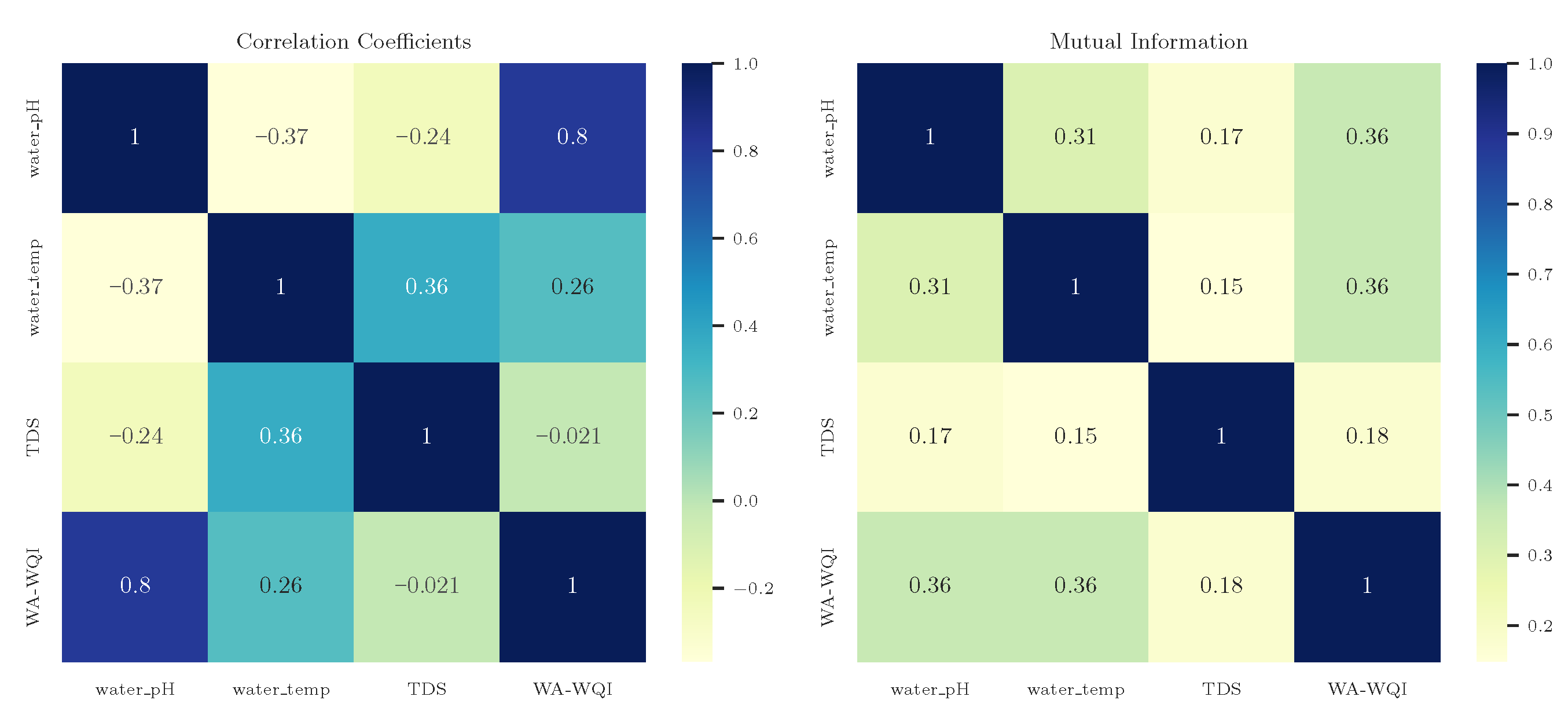
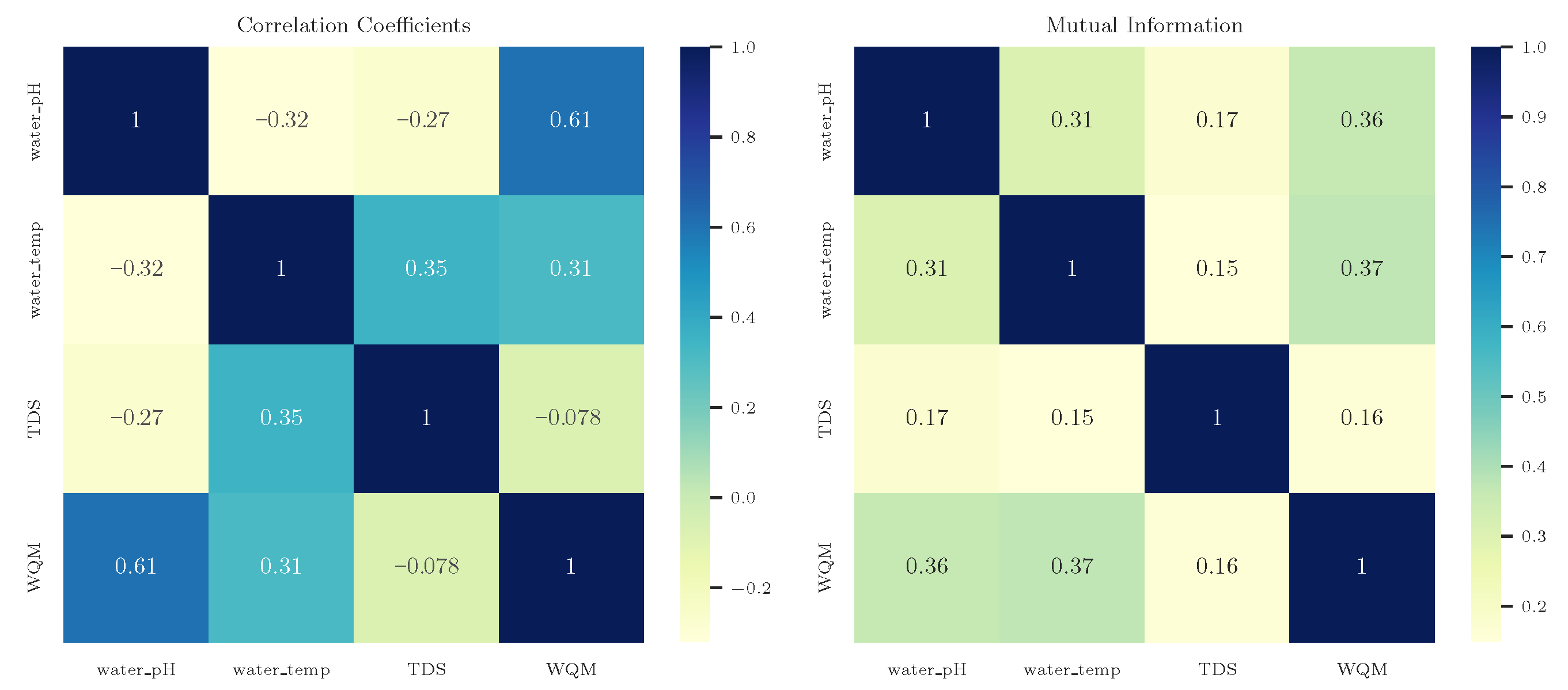
Exploratory Analysis of Variable Relationships

To complement the insights derived from model sparsification, we conducted an exploratory analysis of the pairwise relationships among the input variables (pH, temperature, and TDS) and the corresponding water quality indices (WA-WQI and WQM-WQI). Figure 6 and Figure 7 each present two heatmaps: the left panel reports correlation coefficients, while the right panel displays normalized mutual information (MI). Correlation captures linear or monotonic relationships (using Pearson or Spearman methods, respectively), while MI quantifies both linear and nonlinear dependencies in a normalized range of $[0,1]$. These complementary metrics are widely used for feature relevance analysis in machine-learning workflows [42]. Importantly, these analyses were performed exclusively on the training and validation data to prevent data leakage and ensure the integrity of the final test set evaluation. Pearson correlation was used for the WA-WQI case (reflecting its linear formulation), while Spearman correlation was adopted for the WQM-WQI case to capture potential nonlinear monotonic patterns.

Figure 6 reveals a strong positive correlation between pH and WA-WQI ($r=0.80$), along with a moderate correlation between temperature and WA-WQI ($r=0.26$). In contrast, TDS shows negligible linear correlation with WA-WQI ($r\approx -0.02$), while exhibiting moderate correlations with pH ($r=-0.24$) and temperature ($r=0.36$). These patterns are further supported by the mutual information (MI) matrix, which indicates moderate shared information between WA-WQI and both pH and temperature (MI = 0.36), whereas TDS again demonstrates the lowest relevance (MI = 0.18).

A similar pattern is observed in Figure 7, corresponding to the WQM-WQI case. Here, the strongest correlation is observed between pH and WQM-WQI ($\rho =0.61$), followed by moderate associations between temperature and WQM-WQI ($\rho =0.31$), and between temperature and TDS ($\rho =0.35$). TDS again shows negligible correlation with WQM-WQI ($\rho \approx -0.08$). The MI matrix confirms these observations, highlighting pH and temperature as the most informative variables with respect to WQM-WQI (MI = 0.36 and 0.37, respectively), while TDS again contributes minimal shared information (MI = 0.16).

Taken together, these results support the pruning decisions made by the KAN models. The removal of TDS in the pruned architectures is consistent with its low statistical relevance, as quantified by both correlation and mutual information. Despite being an input in the original WQI formulations, TDS was identified as non-essential through a purely data-driven process—demonstrating KAN’s capacity for implicit feature selection. This finding has practical implications for the design of IoT-based monitoring systems, where sensor minimization can lead to cost reductions and enhanced robustness. The alignment between statistical insights and model behavior further reinforces the interpretability and efficiency of the pruned KAN models.

3.3. Model Inference and Symbolic Expression Evaluation

3.3.1. Symbolic Formulas

For the first case study (WA-WQI prediction), the symbolic expressions extracted from the original and pruned KAN models are presented in Equations (10) and (11), respectively. These expressions describe the learned relationship between the input variables—pH ($x_1$), temperature ($x_2$), and TDS ($x_3$)—and the output WA-WQI (y):

Original model (full):

$$y=17.30x_1+24.41x_2+0.006x_3-684.21$$

(10)

Pruned model:

$$y=17.30x_1+24.41x_2-684.60$$

(11)

The symbolic expressions from both models exhibit close numerical similarity. Notably, TDS ($x_3$) receives a negligible coefficient (0.006) in Equation (10), justifying its removal in the pruned model. The resulting simplified expression in Equation (11) retains the predictive structure, highlighting the model’s capacity to perform implicit feature selection without compromising accuracy.

For the second case study (WQM-WQI prediction), the symbolic expressions extracted from the original and pruned models are considerably more complex due to the nonlinear nature of the target function, as illustrated in Equations (12) and (13). To improve readability, the expressions have been reformatted as follows.

Original model (full):

$$\begin{array}{cc}\hfill y& =-0.002x_1+0.434x_2+0.056x_3\hfill \\ \hfill & +0.03{(1-0.231x_1)}^2\hfill \\ \hfill & +5.534sin(0.015x_1+0.021x_2-0.023x_3+0.585)\hfill \\ \hfill & +2.687\hfill \end{array}$$

(12)

Pruned model:

$$\begin{array}{cc}\hfill y& =\sqrt{0.124{(x_1+0.7979)}^2+1.096{(0.5697x_2+1)}^2+11.77}\hfill \\ \hfill & -4.0626\hfill \end{array}$$

(13)

In these expressions, $x_1$, $x_2$, and $x_3$ correspond to the quality ratings of pH, temperature, and TDS (i.e., $q_{\mathrm{pH}}$, $q_{\mathrm{temp}}$, and $q_{\mathrm{TDS}}$), respectively, and y denotes the WQM-WQI value.

The symbolic expression from the original model (Equation (12)) is clearly more intricate and difficult to associate directly with the mathematical form of WQM-WQI as defined in Equation (2). In contrast, the pruned expression in Equation (13) closely resembles the original WQM-WQI formulation, showcasing the model’s ability to recover a meaningful approximation of the underlying aggregation function. In both case studies, the pruned symbolic KAN models succeeded in extracting interpretable mathematical relationships between the input variables and the target WQI. This highlights their effectiveness not only in prediction but also in model simplification and symbolic recovery of domain-relevant formulations. The next section presents and discusses the performance metrics used to evaluate the prediction models under different configurations.

3.3.2. Performance Evaluation

In the following, we first present the performance metrics and results independently for each case study (WA-WQI and WQM-WQI), followed by a comparative discussion of the general findings that emerged across both formulations.

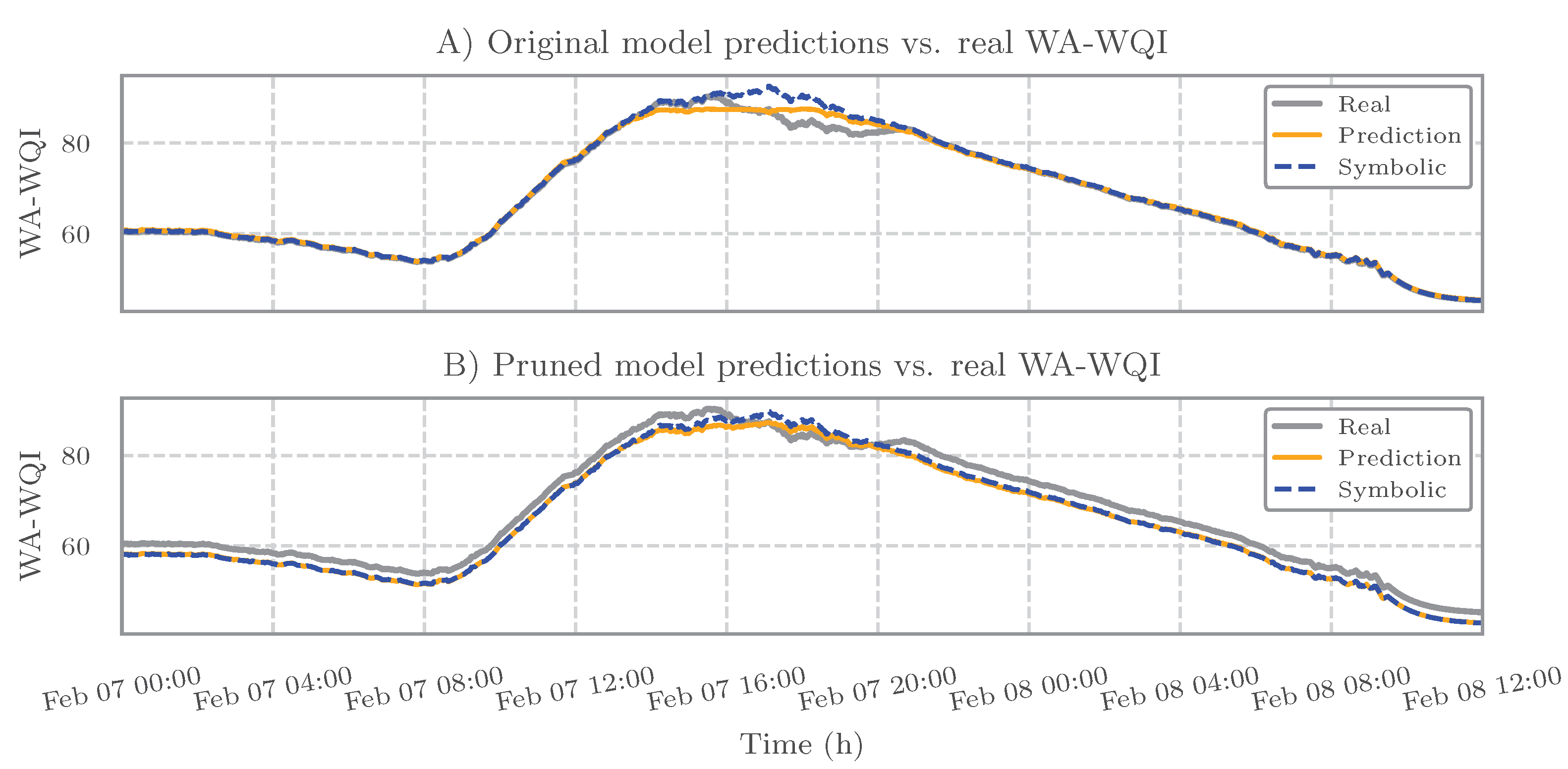
Results for the WA-WQI Case Study

For the WA-WQI prediction, the performance of the trained KAN models and the predictive capacity of the corresponding symbolic expressions are illustrated in Figure 8. The predictions generated by both the original and pruned KAN models exhibit strong agreement with the ground truth values in the test set. Furthermore, the symbolic expressions extracted from each model produce time series that are nearly indistinguishable from their respective model predictions. This high similarity explains the visual overlap observed in Figure 8 and confirms that the symbolic expressions effectively replicate the internal mappings learned by the trained models.

Table 4. Performance metrics on the test set for the WA-WQI case study. The results include the original and pruned KAN models and their corresponding symbolic expressions, evaluated on unseen test data from a classical hold-out validation strategy.

Model	R²	MAE	RMSE
KAN (full) inference	0.994	0.526	0.948
Symbolic (full)	0.986	0.627	1.538
KAN (pruned) inference	0.965	2.322	2.408
Symbolic (pruned)	0.967	2.291	2.330

presents a quantitative assessment of both KAN models and their corresponding symbolic expressions using the coefficient of determination ($R^2$), MAE, and RMSE. The results show that the pruned model, which was trained with a reduced set of input variables, achieves performance comparable to the original model. This is evidenced by similar $R^2$, MAE, and RMSE values for its symbolic version. Notably, the symbolic expressions derived from both models closely approximate the true input–output relationships, when evaluated on test data that were not used during training.

These findings highlight the capacity of the KAN framework to identify and eliminate less relevant variables while preserving predictive accuracy, thereby reinforcing its potential for interpretable and compact symbolic modeling.

Results for the WQM-WQI Case Study

While a classical hold-out validation strategy was adopted for the WA-WQI case study, allowing for a straightforward visualization of model predictions against the test set time series, a more complex evaluation approach was adopted for the WQM-WQI formulation, as described in Section 2.5.2. Specifically, the original and pruned KAN models were trained and validated on data from an earlier period, whereas a distinct segment collected nearly one month later was used for performance evaluation through a 5-fold cross-validation strategy. In addition to the KAN models, fifteen baseline regressors were trained on the original training set. The top three, selected based on their validation performance, were included in the final comparative evaluation. Given the increased complexity of this evaluation setup and the heterogeneity of models and folds, time-series visualizations would offer limited interpretability. Therefore, this section presents only the quantitative performance metrics to summarize and compare model behavior.

Table 5. Performance metrics on the validation set for the WQM-WQI case study. Results include the original and pruned KAN models, their corresponding symbolic expressions, and the top three baseline regressors selected using the LazyPredict Python library.

Model	R²	MAE	RMSE
KAN (full) inference	0.9149	1.7273	2.9471
Symbolic (full)	0.9012	2.0898	3.1761
KAN (pruned) inference	0.9847	0.5848	1.2496
Symbolic (pruned)	0.9997	0.1525	0.1845
MLPRegressor	0.9980	0.2410	0.4530
RandomForestRegressor	0.8820	2.0710	3.4640
BaggingRegressor	0.8800	2.1150	3.4990

presents the performance metrics obtained on the validation set for the WQM-WQI case study. Unlike the WA-WQI formulation, where the original model maintained superior performance, here the pruned KAN model outperformed its original counterpart. This observation suggests that, in scenarios characterized by a complex and nonlinear input–output relationship—as is the case for WQM-WQI—pruning the model and focusing on the most relevant input variables may improve generalization. Future investigations could be directed toward systematically validating this insight. Specifically, the pruned model achieved an $R^2$ value exceeding 0.98, along with a substantial reduction in MAE and RMSE compared to the original version.

Among the baseline models, the MLPRegressor delivered the best performance. This result aligns with the theoretical foundation of multilayer perceptrons (MLPs) as universal function approximators, which makes them particularly effective in modeling nonlinear relationships [19,20]. The random forest and bagging regressors also yielded competitive results. Their performance can be attributed to the ensemble learning principle, in which predictions are derived by aggregating the outputs of multiple individual models trained on different subsets of the data or with varying learning configurations. This collective inference strategy enhances robustness and mitigates overfitting, thereby contributing to the strong generalization capabilities observed in these models [35,43].

Considering the results summarized in Table 5, the pruned KAN model and the top-performing baseline regressors were evaluated on the test set, which consisted of data collected nearly one month after the training period, as detailed in Section 2.5.2. From

Table 6. Performance metrics on the test set for the WQM-WQI case study, reported as mean ± standard deviation across 5-fold cross-validation on a time-shifted test segment. Models include the pruned KAN model and its symbolic expression, along with the top three baseline regressors selected on the validation set.

Model	R²	MAE	RMSE
Symbolic (pruned)	$0.998\pm 0.001$	$0.449\pm 0.166$	$0.685\pm 0.312$
MLPRegressor	$0.996\pm 0.001$	$0.687\pm 0.226$	$1.157\pm 0.266$
KAN (pruned) inference	$0.919\pm 0.100$	$2.764\pm 1.507$	$4.266\pm 2.152$
RandomForestRegressor	$0.904\pm 0.059$	$4.141\pm 0.947$	$5.218\pm 1.021$
BaggingRegressor	$0.902\pm 0.059$	$4.205\pm 0.936$	$5.281\pm 1.002$

, it can be noted that the symbolic expression derived from the pruned KAN model achieved the highest performance, with an $R^2$ of 0.998 and the lowest MAE and RMSE, closely followed by the MLPRegressor, which also demonstrated strong predictive accuracy. This outcome reinforces the symbolic model’s ability to generalize well across time-shifted data.

Notably, the pruned KAN model (inference) did not match the performance of its symbolic counterpart. This discrepancy may be attributed to the fact that the underlying input–output relationship was defined by a known mathematical expression. In such contexts, symbolic regression may offer advantages by more directly capturing the functional structure, benefiting from smoother interpolation. While the pruned model showed competitive performance, the symbolic expression demonstrated even better generalization on temporally shifted test data. Otherwise, the ensemble methods random forest and bagging regressors, exhibited consistent behavior compared to the validation phase, indicating stable generalization performance across temporal variations.

3.4. General Considerations

The findings presented in this study underscore the potential of KAN as interpretable and accurate data-driven models for applications where feature selection and model transparency are essential. The use of a dataset related to aquaponics—a subfield of aquaculture—further emphasizes the practical relevance of this approach, particularly given the critical role that WQI analysis plays in aquaculture operations [44]. Moreover, the proposed pipeline aligns with previous studies in the field that prioritize interpretability and the adoption of straightforward, implementable techniques [45,46].

The competitive performance of the symbolic expressions derived from KAN models highlights the utility of symbolic regression for revealing latent input–output relationships in environmental systems. Notably, the consistent results across both WQI case studies presented in this work validate the flexibility and robustness of the proposed methodology. In this context, the combination of model pruning, symbolic expression extraction, and benchmarking against classical machine-learning models proved effective in delivering interpretable and generalizable solutions applicable to real-world scenarios.

Furthermore, recent studies have shown that KAN models can outperform traditional architectures such as multilayer perceptrons (MLPs) and random forests when modeling complex nonlinear phenomena, as demonstrated in the context of electrohydrodynamic pumping [47]. These results reinforce the relevance of KANs in scientific and technological domains where high predictive accuracy must be complemented by model interpretability.

3.5. KAN Limitations and Challenges

Despite their promising features, KANs also present several limitations and challenges that must be acknowledged. One of their main advantages—interpretability—can be considered partial or dependent on the specific application. In fields like computer vision or natural language processing, the symbolic expressions generated by KANs often contribute little to understanding how predictions are made [48]. Additionally, although KANs produce symbolic approximations using splines and regression, they do not offer the same explicit, rule-based logic provided by tree-based models. Tree-based models generate interpretable “if-then” rules that clearly map features to decisions, which is particularly important in areas like healthcare or finance where decision traceability is essential. To address this gap, KANs can be paired with post hoc explanation methods such as SHapley Additive exPlanations (SHAP) or LIME [49,50]. These tools help explain individual predictions (local explanations) and overall model behavior (global insights) without requiring any changes to the trained model [48].

Another important limitation of KANs concerns their computational cost. When applied to high-dimensional datasets, KAN models may become less efficient due to the increased complexity of their architecture. This added complexity impacts both optimization and training time, making them less practical in scenarios that demand fast computation or operate on large-scale data. In contrast, simpler neural networks such as MLPs are often more computationally efficient and easier to train, particularly in large-scale or resource-constrained environments. In summary, while KANs offer a promising combination of model expressiveness and interpretability, further research is needed to improve their scalability, transparency, and adaptability across different tasks. Addressing these challenges will be essential for the broader adoption of KANs in industrial and real-world applications.

4. Conclusions

This study evaluated the use of Kolmogorov–Arnold Networks (KAN) for modeling two formulations of the water quality index (WQI): the weighted arithmetic WQI (WA-WQI) and the weighted quadratic mean WQI (WQM-WQI), considered as independent case studies. Both indices were derived as linear and nonlinear combinations, respectively, of normalized water quality parameters—pH, total dissolved solids (TDS), and temperature—collected from an IoT-enabled aquaponic system. For each case, two KAN models were developed: a full-input model using all three variables and a pruned model employing only pH and temperature. The pruning process, guided by sparsification, aligned with the results of correlation and mutual information analyses, which indicated TDS as the least relevant input. This convergence supports the robustness of the feature selection approach adopted.

In terms of predictive performance, both trained KAN models and their corresponding symbolic expressions closely approximated the true WQI values. In the WA-WQI case, a hold-out validation strategy was used to demonstrate the pipeline’s behavior and interpretability under controlled conditions. In contrast, the WQM-WQI case employed 5-fold cross-validation on a temporally disjoint test set, providing a more realistic assessment of generalization to unseen data. The pruned symbolic KAN models consistently matched or outperformed the full models and top baseline regressors, achieving $R^2$ scores exceeding 0.96 across all cases. These results confirm that input reduction did not compromise performance and, in some scenarios, improved model generalization. Additionally, the extracted symbolic expressions offer interpretable representations that align with application-specific requirements.

Overall, the proposed KAN-based pipeline—comprising training, pruning, symbolic expression extraction, and benchmarking—proved effective for building accurate, compact, and interpretable models. The pruned KAN models are particularly well-suited for deployment in aquaculture monitoring, where minimizing sensor requirements without sacrificing accuracy can reduce operational complexity and cost. Future work could explore the application of KANs in more complex tasks such as classification, multivariate forecasting, or modeling with higher-dimensional inputs. Further evaluation using longer time series and diverse environmental conditions may enhance understanding of the generalizability and practical limitations of KAN-based symbolic models across environmental and industrial monitoring domains.

References

1. Liu, Z.; Wang, Y.; Vaidya, S.; Ruehle, F.; Halverson, J.; Soljačić, M.; Hou, T.Y.; Tegmark, M. KAN: Kolmogorov-Arnold Networks. arXiv 2024, arXiv:2404.19756. [Google Scholar] [CrossRef]
2. Liu, Z.; Ma, P.; Wang, Y.; Matusik, W.; Tegmark, M. KAN 2.0: Kolmogorov-Arnold Networks Meet Science. arXiv 2024, arXiv:2408.10205. [Google Scholar] [CrossRef]
3. Ji, T.; Hou, Y.; Zhang, D. A Comprehensive Survey on Kolmogorov Arnold Networks (KAN). arXiv 2024, arXiv:2407.11075. [Google Scholar] [CrossRef]
4. Gilbert Zequera, R.A.; Rassõlkin, A.; Vaimann, T.; Kallaste, A. Kolmogorov-Arnold networks for algorithm design in battery energy storage system applications. Energy Rep. 2025, 13, 2664–2677. [Google Scholar] [CrossRef]
5. Huang, Y.; Li, B.; Wu, Z.; Liu, W. Symbolic Regression Based on Kolmogorov–Arnold Networks for Gray-Box Simulation Program with Integrated Circuit Emphasis Model of Generic Transistors. Electronics 2025, 14, 1161. [Google Scholar] [CrossRef]
6. Siswanto, B.; Dani, Y.; Morika, D.; Mardiyana, B. A simple dataset of water quality on aquaponic fish ponds based on an internet of things measurement device. Data Brief 2023, 48, 109248. [Google Scholar] [CrossRef]
7. Uddin, M.G.; Nash, S.; Olbert, A.I. A review of water quality index models and their use for assessing surface water quality. Ecol. Indic. 2021, 122, 107218. [Google Scholar] [CrossRef]
8. Chidiac, S.; El Najjar, P.; Ouaini, N.; El Rayess, Y.; El Azzi, D. A comprehensive review of water quality indices (WQIs): History, models, attempts and perspectives. Rev. Environ. Sci. Bio/Technol. 2023, 22, 349–395. [Google Scholar] [CrossRef]
9. Chicco, D.; Warrens, M.J.; Jurman, G. The coefficient of determination R-squared is more informative than SMAPE, MAE, MAPE, MSE and RMSE in regression analysis evaluation. PeerJ Comput. Sci. 2021, 7, e623. [Google Scholar] [CrossRef]
10. Krishnamurthi, R.; Kumar, A.; Gopinathan, D.; Nayyar, A.; Qureshi, B. An Overview of IoT Sensor Data Processing, Fusion, and Analysis Techniques. Sensors 2020, 20, 6076. [Google Scholar] [CrossRef]
11. Liu, Y.; Dillon, T.; Yu, W.; Rahayu, W.; Mostafa, F. Missing Value Imputation for Industrial IoT Sensor Data with Large Gaps. IEEE Internet Things J. 2020, 7, 6855–6867. [Google Scholar] [CrossRef]
12. França, C.M.; Couto, R.S.; Velloso, P.B. Missing Data Imputation in Internet of Things Gateways. Information 2021, 12, 425. [Google Scholar] [CrossRef]
13. James, G.; Witten, D.; Hastie, T.; Tibshirani, R.; Taylor, J. Resampling Methods. In An Introduction to Statistical Learning; Springer International Publishing: Berlin/Heidelberg, Germany, 2023; pp. 201–228. [Google Scholar] [CrossRef]
14. Xu, Y.; Goodacre, R. On Splitting Training and Validation Set: A Comparative Study of Cross-Validation, Bootstrap and Systematic Sampling for Estimating the Generalization Performance of Supervised Learning. J. Anal. Test. 2018, 2, 249–262. [Google Scholar] [CrossRef] [PubMed]
15. Cao, L. Practical Issues in Implementing a Single-Pole Low-Pass IIR Filter [Applications Corner]. IEEE Signal Process. Mag. 2010, 27, 114–117. [Google Scholar] [CrossRef]
16. Uddin, M.G.; Nash, S.; Rahman, A.; Olbert, A.I. A comprehensive method for improvement of water quality index (WQI) models for coastal water quality assessment. Water Res. 2022, 219, 118532. [Google Scholar] [CrossRef]
17. Patel, D.D.; Mehta, D.J.; Azamathulla, H.M.; Shaikh, M.M.; Jha, S.; Rathnayake, U. Application of the Weighted Arithmetic Water Quality Index in Assessing Groundwater Quality: A Case Study of the South Gujarat Region. Water 2023, 15, 3512. [Google Scholar] [CrossRef]
18. Abdolazizi, K.P.; Aydin, R.C.; Cyron, C.J.; Linka, K. Constitutive Kolmogorov–Arnold Networks (CKANs): Combining accuracy and interpretability in data-driven material modeling. J. Mech. Phys. Solids 2025, 203, 106212. [Google Scholar] [CrossRef]
19. Hornik, K.; Stinchcombe, M.; White, H. Multilayer feedforward networks are universal approximators. Neural Netw. 1989, 2, 359–366. [Google Scholar] [CrossRef]
20. Leshno, M.; Lin, V.Y.; Pinkus, A.; Schocken, S. Multilayer feedforward networks with a nonpolynomial activation function can approximate any function. Neural Netw. 1993, 6, 861–867. [Google Scholar] [CrossRef]
21. Schmidt-Hieber, J. The Kolmogorov–Arnold representation theorem revisited. Neural Netw. 2021, 137, 119–126. [Google Scholar] [CrossRef]
22. Vaca-Rubio, C.J.; Blanco, L.; Pereira, R.; Caus, M. Kolmogorov-Arnold Networks (KANs) for Time Series Analysis. arXiv 2024, arXiv:2405.08790. [Google Scholar] [CrossRef]
23. Abueidda, D.W.; Pantidis, P.; Mobasher, M.E. DeepOKAN: Deep operator network based on Kolmogorov Arnold networks for mechanics problems. Comput. Methods Appl. Mech. Eng. 2025, 436, 117699. [Google Scholar] [CrossRef]
24. Perperoglou, A.; Sauerbrei, W.; Abrahamowicz, M.; Schmid, M. A review of spline function procedures in R. BMC Med. Res. Methodol. 2019, 19, 46. [Google Scholar] [CrossRef] [PubMed]
25. Hasan, M.S.; Alam, M.N.; Fayz-Al-Asad, M.; Muhammad, N.; Tunç, C. B-spline curve theory: An overview and applications in real life. Nonlinear Eng. 2024, 13, 20240054. [Google Scholar] [CrossRef]
26. Joseph, V.R. Optimal ratio for data splitting. Stat. Anal. Data Mining Asa Data Sci. J. 2022, 15, 531–538. [Google Scholar] [CrossRef]
27. Kapoor, S.; Narayanan, A. Leakage and the reproducibility crisis in machine-learning-based science. Patterns 2023, 4, 100804. [Google Scholar] [CrossRef]
28. Goap, A.; Sarkar, S.; Roy, A.; Krishna, C.R.; Kumar, S. An IoT-Based Architectural Framework for Earthquake Warning System Using Low-cost Heterogeneous Seismic Sensors. Arab. J. Sci. Eng. 2025, 1–16. [Google Scholar] [CrossRef]
29. Eldin Rashed, A.E.; Elmorsy, A.M.; Mansour Atwa, A.E. Comparative evaluation of automated machine learning techniques for breast cancer diagnosis. Biomed. Signal Process. Control. 2023, 86, 105016. [Google Scholar] [CrossRef]
30. Salehin, I.; Islam, M.S.; Saha, P.; Noman, S.; Tuni, A.; Hasan, M.M.; Baten, M.A. AutoML: A systematic review on automated machine learning with neural architecture search. J. Inf. Intell. 2024, 2, 52–81. [Google Scholar] [CrossRef]
31. LazyPredict Python Library. Available online: https://lazypredict.readthedocs.io/en/latest/ (accessed on 25 June 2025).
32. Pedregosa, F.; Varoquaux, G.; Gramfort, A.; Michel, V.; Thirion, B.; Grisel, O.; Blondel, M.; Prettenhofer, P.; Weiss, R.; Dubourg, V.; et al. Scikit-learn: Machine Learning in Python. J. Mach. Learn. Res. 2011, 12, 2825–2830. [Google Scholar]
33. James, G.; Witten, D.; Hastie, T.; Tibshirani, R.; Taylor, J. Linear Regression. In An Introduction to Statistical Learning; Springer International Publishing: Berlin/Heidelberg, Germany, 2023; pp. 69–134. [Google Scholar] [CrossRef]
34. James, G.; Witten, D.; Hastie, T.; Tibshirani, R.; Taylor, J. Tree-Based Methods. In An Introduction to Statistical Learning; Springer International Publishing: Berlin/Heidelberg, Germany, 2023; pp. 331–366. [Google Scholar] [CrossRef]
35. Zhang, Y.; Liu, J.; Shen, W. A Review of Ensemble Learning Algorithms Used in Remote Sensing Applications. Appl. Sci. 2022, 12, 8654. [Google Scholar] [CrossRef]
36. Rodriguez-Galiano, V.; Sanchez-Castillo, M.; Chica-Olmo, M.; Chica-Rivas, M. Machine learning predictive models for mineral prospectivity: An evaluation of neural networks, random forest, regression trees and support vector machines. Ore Geol. Rev. 2015, 71, 804–818. [Google Scholar] [CrossRef]
37. Sanyal, S.; Zhang, P. Improving Quality of Data: IoT Data Aggregation Using Device to Device Communications. IEEE Access 2018, 6, 67830–67840. [Google Scholar] [CrossRef]
38. Herrera, M.; Sasidharan, M.; Merino, J.; Parlikad, A.K. Handling Irregularly Sampled IoT Time Series to Inform Infrastructure Asset Management. IFAC-PapersOnLine 2022, 55, 241–245. [Google Scholar] [CrossRef]
39. Harker, M.; Rath, G. System Identification with Non-Uniformly Sampled and Intermittent Data in the Internet of Things. In Proceedings of the 2023 International Conference on Applied Electronics (AE), Pilsen, Czech Republic, 6–8 September 2023; pp. 1–6. [Google Scholar] [CrossRef]
40. Alotaibi, O.; Pardede, E.; Tomy, S. Cleaning Big Data Streams: A Systematic Literature Review. Technologies 2023, 11, 101. [Google Scholar] [CrossRef]
41. Hu, H.; Huang, S. A Kalman Filtering and Least Absolute Residuals based Time Series Data Reconstruction Strategy for Structural Health Monitoring. In Proceedings of the 2024 IEEE 10th World Forum on Internet of Things (WF-IoT), Ottawa, QC, Canada, 10–13 November 2024; pp. 1–6. [Google Scholar] [CrossRef]
42. Zhou, H.; Wang, X.; Zhu, R. Feature selection based on mutual information with correlation coefficient. Appl. Intell. 2022, 52, 5457–5474. [Google Scholar] [CrossRef]
43. N., G.; Jain, P.; Choudhury, A.; Dutta, P.; Kalita, K.; Barsocchi, P. Random Forest Regression-Based Machine Learning Model for Accurate Estimation of Fluid Flow in Curved Pipes. Processes 2021, 9, 2095. [Google Scholar] [CrossRef]
44. Do, D.D.; Le, A.H.; Vu, V.V.; Le, D.A.N.; Bui, H.M. Evaluation of water quality and key factors influencing water quality in intensive shrimp farming systems using principal component analysis-fuzzy approach. Desalin. Water Treat. 2025, 321, 101002. [Google Scholar] [CrossRef]
45. Ferreira, N.; Bonetti, C.; Seiffert, W. Hydrological and Water Quality Indices as management tools in marine shrimp culture. Aquaculture 2011, 318, 425–433. [Google Scholar] [CrossRef]
46. Tallar, R.Y.; Suen, J.P. Aquaculture Water Quality Index: A low-cost index to accelerate aquaculture development in Indonesia. Aquac. Int. 2015, 24, 295–312. [Google Scholar] [CrossRef]
47. Peng, Y.; Wang, Y.; Hu, F.; He, M.; Mao, Z.; Huang, X.; Ding, J. Predictive modeling of flexible EHD pumps using Kolmogorov–Arnold Networks. Biomim. Intell. Robot. 2024, 4, 100184. [Google Scholar] [CrossRef]
48. Somvanshi, S.; Javed, S.A.; Islam, M.M.; Pandit, D.; Das, S. A Survey on Kolmogorov-Arnold Network; ACM Computing Surveys: New York, NY, USA, 2025. [Google Scholar] [CrossRef]
49. Ribeiro, M.T.; Singh, S.; Guestrin, C. “Why Should I Trust You?”: Explaining the Predictions of Any Classifier. In Proceedings of the 22nd ACM SIGKDD International Conference on Knowledge Discovery and Data Mining, San Francisco, CA, USA, 13–17 August 2016; KDD’16. ACM Computing Surveys: New York, NY, USA, 2016; pp. 1135–1144. [Google Scholar] [CrossRef]
50. Lundberg, S.M.; Lee, S.I. A unified approach to interpreting model predictions. In Proceedings of the 31st International Conference on Neural Information Processing Systems, Long Beach, CA, USA, 4–9 December 2017; NIPS’17. Curran Associates Inc.: Red Hook, NY, USA, 2017; pp. 4768–4777. [Google Scholar]
Figure 1. Flowchart of the proposed methodology. The pipeline was applied consistently across both study cases and includes data preprocessing, KAN model training, symbolic regression, and model evaluation.
J 08 00024 g001
Figure 2. Effect of preprocessing on pH signal. (A) Comparison between original raw data and preprocessed signal. (B) Zoomed view highlighting a segment with missing values in the raw signal and their imputation. (C) Additional zoomed view illustrating the noise attenuation achieved by smoothing.
J 08 00024 g002
Figure 3. Time series of water quality variables (pH, TDS, and temperature) and the WA-WQI over the study period. The WA-WQI plot highlights the training, validation, and test intervals used in the hold-out data split.
J 08 00024 g003
Figure 4. Structure of the original (left) and pruned (right) KAN models used for WA-WQI prediction. Darker nodes and edges indicate active components retained after sparsification.
J 08 00024 g004
Figure 5. Structure of the original (left) and pruned (right) KAN models used for WQM-WQI prediction. Darker nodes and edges indicate active components retained after sparsification.
J 08 00024 g005
Figure 6. (Left): Pearson correlation coefficients among water quality variables and WA-WQI. (Right): Normalized mutual information (MI), symmetrized and scaled to [ 0 , 1 ] .
J 08 00024 g006
Figure 7. (Left): Spearman correlation coefficients among water quality variables and WQM-WQI. (Right): Normalized mutual information (MI), symmetrized and scaled to [ 0 , 1 ] .
J 08 00024 g007
Figure 8. Comparison of predictions and symbolic expressions against the real WA-WQI values over the test period. (A) Results from the original model show a good match between predicted and symbolic values. (B) The pruned model and its symbolic expression exhibit an almost identical output, reflecting the model’s convergence to a simplified but highly accurate analytical form. This result highlights the ability of KAN to recover interpretable expressions with minimal loss in performance.
J 08 00024 g008