Depicting Falsifiability in Algebraic Modelling

Abstract

This paper investigates how algebraic structures can encode epistemic limitations, with a focus on object properties and measurement. Drawing from philosophical concepts such as underdetermination, we argue that the weakening of algebraic laws can reflect foundational ambiguities in empirical access. Our approach supplies instruments that are necessary and sufficient towards practical falsifiability. Besides introducing this new concept, we consider, exemplarily and as a starting point, the following two fundamental algebraic laws in more detail: the associative law and the commutative law. We explore and analyze weakened forms of these laws. As a mathematical feature, we demonstrate that the existence of a weak neutral element leads to the emergence of several transversal algebraic laws. Most laws are individually weaker than the combination of associativity and commutativity, but many pairs of two laws are equivalent to this combination. We also show that associativity and commutativity can be combined to a simple, single law, which we call cyclicity. We illustrate our approach with many tables and practical examples.

1. Introduction

Scientific practice is shaped not only by experimental techniques and data but also by the profound philosophical questions concerning what can be known and how that knowledge can be interpreted. The aim of this paper is to investigate how algebraic structures, especially in a weakened form, can serve as a formal counterpart to epistemic constraints encountered in the empirical sciences.

1.1. Mathematical Framework

Let x and y be two objects that can be combined via a dyadic operand, denoted by +. There are two ways to apply this operand to x and y, namely

$$\begin{array}{c}\hfill x+y\mathrm{and}y+x.\end{array}$$

The objects x and y are said to commute if $x+y=y+x$.

We now shift from a mathematical to a more physical perspective. From this standpoint, the expressions $x+y$ and $y+x$ are accessible only through measurements. Let M denote such a (possibly multivariate) measurement. If x and y commute, then we have that

$$\begin{array}{c}\hfill M(x+y)=M(y+x).\end{array}$$

(1)

The converse holds only if the measurement function M is sufficiently expressive. Notable contributions in the philosophy of science, such as Willard Van Orman Quine’s notion of underdetermination [1] and the Copenhagen interpretation of quantum mechanics, suggest that measurement functions are generally not expressive enough to establish the identity. So, even if the best possible M is chosen, algebra may add auxiliary hypotheses [2], namely, that $x+y$ is identical to $y+x$, although we only observe this commutativity by all of the measurements. In such cases, the algebraic representation becomes unfalsifiable from a captious perspective and, according to Karl Popper [3], should be replaced by a testable formulation like Equation (1). Equation (1) itself is algebraically too weak, as a law should persist, at least to some extend, in more complicated calculations. Hence, we propose that

$$\begin{array}{c}\hfill M(a+(x+y)+b)=M(a+(y+x)+b)\end{array}$$

(2)

shall be satisfied for all relevant objects a and b. The objects a and b have a weak interpretation as an “environment”. Clearly, commuting objects satisfy (2). Since M can be chosen arbitrarily, a broad spectrum of philosophical interpretations and specifications are possible.

In our approach, the mathematical implications heavily rely on the following additional assumption: the existence of a weak form of a neutral element. Since the theoretical presence or absence of such an element is often non-critical, this assumption is considered as reasonable for the mathematical statements. Some of the examples below demonstrate that a weak neutral element may not exist.

1.2. Overview

Section 2 illustrates the philosophical aspects of our algebraic approach. Section 3 introduces the new concept with various illustrative practical examples and tables that exemplify the theoretical aspects. Several remarks and propositions depict mathematical examples and properties. Theorem 4 in Section 4 demonstrates that under weakened assumptions, associativity and commutativity can be expressed in many equivalent formulations. Furthermore, we show that certain algebraic identities hold under weaker assumptions than hitherto used. For instance, Theorem 1 shows that in case of hemi-associativity, parentheses can always be removed. Proofs are deferred to Section 5 and Section 6. Section 7 connects our findings to the relevant literature in algebra, including a brief presentation of the origins of the technical terms.

2. Philosophical Aspects

2.1. Underdetermination

The underdetermination thesis states that, for any finite set of empirical data, there may exist multiple, logically distinct theories that are equally compatible with it. In addition, objects that are different, but not really distinguishable, give rise to quotient structures in mathematics. Our approach can be considered as an alternative if quotient spaces are not productive. Particularly, our function M allows for a more flexible modeling of the coarse granularity of empirical observations.

2.2. Falsifiability

A central concern in philosophy of science is the criterion of falsifiability, most famously articulated by Karl Popper. A theory is empirically meaningful only if it makes predictions that can, in principle, be refuted by observation. Algebraically, falsifiability requires a theory that differentiates precisely between possible outcomes (and not more). In particular, a structure that in a hidden form introduces distinctions unsupported by empirical measurements might be inadequate.

2.3. Theses

We propose that the following algebraic features are necessary for empirical falsifiability: (i) operations shall respect empirically accessible domains, (ii) operations shall produce distinguishable results for distinguishable outputs; and (iii) failure of global identities that are not supported by the empirical context. Since, in our framework, distinguishability is allowed to be context dependent, we postulate this also from a philosophical point of view.

3. Notions

In the sequel we always understand $x+y+z$ as $(x+y)+z$. We use the prefix “hemi” to indicate that we use a kind of weak form of a certain property.

For an overview and a better understanding,

Table 1. Important symbols and their meaning.

Symbol	Mathematical Meaning	Interpretation and Examples
+	any dual operand	“adding” also in the popular or broad sense, e.g.: adding a chemical substance to another union of two sets
G	any ensemble of objects	the ensemble of objects of the same type we deal with: chemical substances harvest on different plantations
$G_s$	a subset of G that contains the hemi-right-neutral elements	see $G_e$; the distinction between $G_s$ and $G_e$ is purely mathematical
$G_e$	subset of $G_s$: set of hemi-neutral elements	typical hemi-neutral elements are “nothing” or “zero”, but could be anything with “no effect” or “no value” (in a very broad sense): in chemistry: sometimes water, air, waiting a period of time a poor harvest
$x,y,z$	elements of G	important objects, e.g., in chemistry: the substances that react primarily
$a,b$	elements of G	objects that model the “environment”, i.e., that can be added to the “product”, e.g., in chemistry: solvents, precipitating agents
$\epsilon$	element of $G_e$	hemi-neutral element that is necessary to perform a proof or to give a statement
$\delta$	element of $G_e$	sole purpose is to increase the number of objects in a mathematical term to meet the correct number of elements to apply an equation or a definition
M	a function from G into any arbitrary image set	measurement or the relevant properties of an object
$x⧦y$	$M\left(x\right)=M\left(y\right)$	objects do not differ in important properties or in their measured values

gives a summary of the symbols that are used hereafter and provides some interpretations.

Definition 1. 

Let G and S be non-empty sets. Let $+:G\times G\to G$ be a dyadic operand on G and $M:G\to S$ a map. Denote $M\left(x\right)=M\left(y\right)$ by $x⧦y$ and let

$$\begin{array}{c}\hfill G_s=\{\epsilon \in G:x+\epsilon ⧦x\forall x\in G\}.\end{array}$$

(3)

If $G_s$ is not empty and closed with respect to +, i.e., $\epsilon ,\tilde{\epsilon }\in G_s$ implies $\epsilon +\tilde{\epsilon }\in G_s$, then the tuple $(G,+,M)$ is called a hemi-right-unital magma.

Definition 2. 

Let $(G,+,M)$ be a hemi-right-unital magma. An element $\epsilon \in G_s$ is called a hemi-neutral element if

$$\begin{array}{ccc}\hfill \epsilon +x& ⧦& x\forall x\in G.\hfill \end{array}$$

(4)

We denote the set of all hemi-neutral elements by $G_e$.

In contrast to $G_s$, we do not assume that $G_e$ is closed with respect to +.

Example 1 

(Hemi-neutral elements: pearl oysters). A practical example that might show the appearance of hemi-neutral elements are (unopened) pearl oysters. The value M of a set A of pearl oysters is given by the number of pearls inside. Let + be the union of two sets. Then, the empty set ∅ is the only truly neutral element for unions. Any set ε of empty oysters is a hemi-neutral element with respect to M, i.e., $\epsilon \in G_e$. In case M measures the amount of work needed to open the oysters, then $G_e=\{\varnothing \}$.

Remark 1. 

In probability theory and mathematical statistics, the terms “deterministic” and “constant almost surely” are usually considered undistinguishable neutral elements, since the theory focuses on measurable functions f applied to a random variable X, i.e., $f\left(X\right(\omega \left)\right)$, where $\omega \in \Omega$ and Ω denotes a probability space, i.e., $X\left(\omega \right)$ as a realization of X. Quantum computing deals with functionals f of a random variable as it deals with rotations of unit vectors. Applying a functional f to X is mathematically $\left(f\right(X\left)\right)\left(\omega \right)$, hence an almost surely constant random variable can, in principle, be turned into a random variable with any arbitrary property. The distinction between $f\left(X\right(\omega \left)\right)$ and $\left(f\right(X\left)\right)\left(\omega \right)$ (and the non-acceptance of the latter) might be considered, from a simplistic mathematical point of view, as a key difference between the EPR approach [4] and modern quantum mechanics, cf. quantum contextuality. Ref. [5] mentions that a refined approach to the set $G_e$ may lead to an abstract unified treatment of both situations.

Remark 2. 

Let two (real-valued) random variables, X and Y, have the same distribution. In many cases, we may consider X and Y as indistinguishable, i.e., $X⧦Y$. However, they can be distinguished, if they are both related to a third random variable Z and the correlation is different. Then, $X+Z⧦/ Y+Z$, in general. This shows that the concept “$⧦$” includes a limited range of validity as its definition suggests. This is an advantage of our approach, since otherwise the limited validity is just not that explicit.

Remark 3. 

Of great importance in mathematics are magmas that consist of transformations, where + models the concatenation. In the sprit of [6], Ref. [5] pleads for replacing the general definition of a statistical model by a transformation magma, whose operands obey some kind of hemi-laws.

The smallest hemi-right-unital magma has one element and is trivial. Among the magmas with two elements, only two magmas are non-trivial—the boolean semi-group of the logical or-operator, and the addition within the binary Galois field, see Figure 1. Both operands are associative and commutative. Hence, any unitary magma needs at least three elements to show subtle properties. Subsequently, all magmas have minimal size with the respective property, unless stated otherwise.

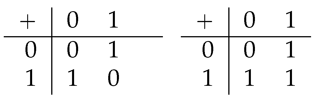
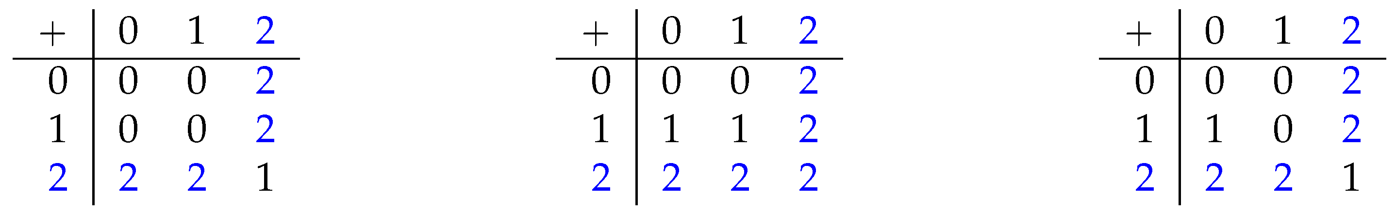
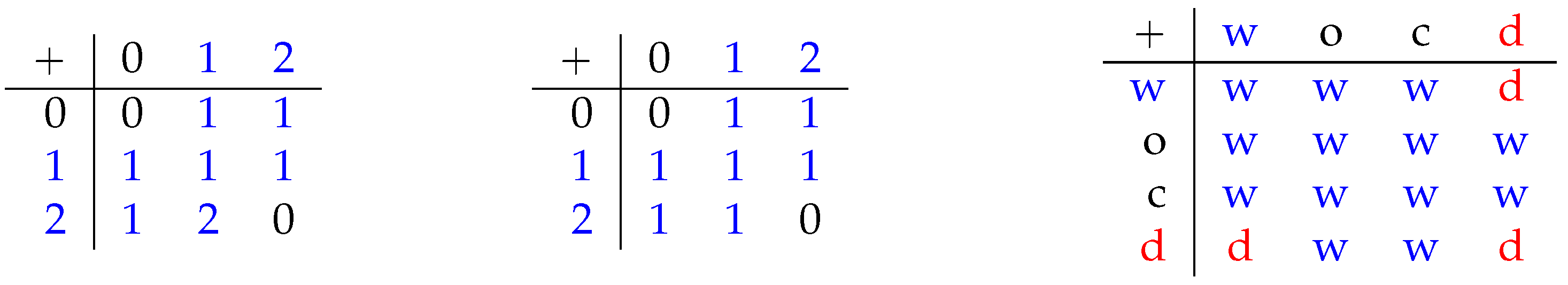
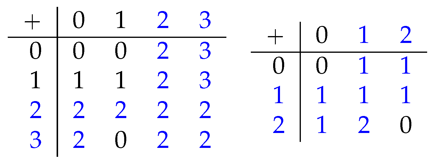
3.1. Hemi-Associativity and Hemi-Commutativity

Definition 3. 

Let $(G,+,M)$ be a hemi-right-unital magma. The operand + is called hemi-associative, if

$$\begin{array}{ccc}\hfill a+\left(\right(x+y)+z)+b& ⧦& a+(x+(y+z\left)\right)+b,\forall a,b,x,y,z\in G,\hfill \end{array}$$

(5)

and hemi-commutative, if

$$\begin{array}{ccc}\hfill a+(y+x)+b& ⧦& a+(x+y)+b\forall a,b,x,y\in G.\hfill \end{array}$$

(6)

It is easily checked that genuine associativity implies Equation (5) and genuine commutativity implies Equation (6). The reverse is not true, as Figure 2 shows.

Example 2 

(Hemi-associativity and hemi-commutativity: pickles). In a production line for pickles, the glasses are filled automatically with cucumbers, where half-filled glasses ought to be removed and reworked manually. A toy model may include the merge of two production lines (denoted by φ below), the sequential production (denoted by ∘), as well as the partial withdrawal of some of the half-filled glasses (denoted by ψ). The measure of interest are the automatically produced glasses of pickles. Mathematically, we might define the following model. Let G be the set of finite sequences of the symbols □ (filled glass) and ⋄ (half-filled glass) including the empty set ∅ (no glass). For elements $g=g_1{g}_2\dots g_n,h=h_1{h}_2\dots h_m\in G$, we define

$$\begin{array}{ccc}\hfill M\left(g\right)& =& \left|\right\{i\in \{1,\dots ,n\}\mid g_i=\square \left\}\right|,\hfill \\ \hfill g\circ h& =& g_1\dots g_n{h}_1\dots h_m,\hfill \\ \hfill \phi (g,h)& =& \left\{\begin{array}{cc}{g}_1{h}_1{g}_2{h}_2\dots g_m{h}_m{g}_{m+1}\dots g_n,\hfill & n>m\hfill \\ g_1{h}_1{g}_2{h}_2\dots g_n{h}_n{h}_{n+1}\dots h_m,\hfill & n\le m\hfill \end{array}\right..\hfill \end{array}$$

We define

$$\begin{array}{ccc}\hfill \psi \left(g\right)& =& {◯}_{i=1}^{n/2}\left\{\begin{array}{cc}\diamond ,\hfill & g_{2i-1}{g}_{2i}=\diamond \diamond \hfill \\ g_{2i-1}{g}_{2i},\hfill & else\hfill \end{array}\right.,neven,\hfill \\ \hfill \psi \left(g\right)& =& \psi (g_1\dots g_{n-1})\circ g_n,nodd,\hfill \\ \hfill \psi (\varnothing )& =& \varnothing .\hfill \end{array}$$

Finally, we establish $g+h=\psi \left(\phi \right(g,h\left)\right)$. For instance,

$$\square \diamond \diamond +\diamond \square \diamond \square =\psi (\square \diamond \diamond \square \diamond \diamond \square )=\square \diamond \diamond \square \diamond \square .$$

One can see that $G_e=\{{\diamond }^i\mid i\in {\mathbb{N}}_0\}$, i.e., similar to Example 1, we have infinitely many hemi-neutral elements, while only one genuine neutral element exists. Note that the operand + is both hemi-associative and hemi-commutative but neither associative nor commutative.

Example 3 

(Associativity without commutativity: rotation). Non-commutative operations, such as matrix multiplication, are frequent in mathematics and physics. Heisenberg’s indeterminacy principle is mathematically a lower bound for the absolute value of a commutator, which is, by definition, zero, if and only if the operation is commutative.

Example 4 

(Hemi-commutativity without hemi-associativity: water treatment). Seventy years ago, the disinfection treatment of water was carried out with chlorine following ozone [7], see also [8]. Although many countries avoid chlorine nowadays, we consider here a model that consists of slightly contaminated water, water enriched with ozone, and water enriched with chlorine. The latter two will eventually reach drinking quality, as ozone and chlorine slowly dissipate. Since both ozone and chlorine are strong oxidants, they can disinfect contaminated water. So in this theoretical example, we assume that mixing the contaminated water with one of the dissolutions, we obtain drinkable water. Here, and in contrast to Example 8 below, the mixing is insensitive to commutation. As advised in the 1950s, we may apply them consecutively. However, first mixing the dissolutions together yields the following two reactions,

$$\begin{array}{ccc}\hfill \mathrm{O}{\mathrm{Cl}}^{-}+{\mathrm{O}}_3& \to & {\mathrm{Cl}}^{-}+2{\mathrm{O}}_2\hfill \\ \hfill 2\mathrm{O}{\mathrm{Cl}}^{-}+2{\mathrm{O}}_3& \to & 2\mathrm{Cl}{\mathrm{O}}_3^{-}+{\mathrm{O}}_2\hfill \end{array}$$

where the hypochlorite $\mathrm{O}{\mathrm{Cl}}^{-}$ stems from

$${\mathrm{Cl}}_2+{\mathrm{H}}_2\mathrm{O}\to \mathrm{O}{\mathrm{Cl}}^{-}+2{\mathrm{H}}^{+}+{\mathrm{Cl}}^{-}.$$

Three quarters of the hypochlorite are transformed into chloride ${\mathrm{Cl}}^{-}$ and one quarter into chlorate $\mathrm{Cl}{\mathrm{O}}_3^{-}$ [9]. The hydrochloric acid turns the water slightly acid and the chlorate is a weak oxidant. This mixture will not safely disinfect contaminated water. So mixing the three liquids is not associative with respect to water quality. Figure 3 presents the corresponding mathematical model.

Theorem 1. 

Let $(G,+,M)$ be a hemi-right-unital magma and $G_e\ne \varnothing$ and + be hemi-associative. Then, all parentheses in a mathematical term can be removed.

Theorem 2. 

Let $(G,+,M)$ be a hemi-right-unital magma and $G_e\ne \varnothing$ and + be hemi-associative and hemi-commutative. Then, in any algebraic expression, the terms can be permuted arbitrarily. To be more precise, let $n\in \mathbb{N}$ and choose $\sigma \in S_n$, where $S_n$ is the permutation group of n symbols. We have, for any choice of $x_1,\dots ,x_n\in G$,

$$\begin{array}{c}\hfill x_1+x_2+\dots +x_n⧦x_{\sigma \left(1\right)}+x_{\sigma \left(2\right)}+\dots +x_{\sigma \left(n\right)}.\end{array}$$

As a consequence, if the operand + is hemi-commutative and hemi-associative, then the operand obeys any other law given below, in particular hemi-right-cyclicity, hemi-left-cyclicity, hemi-right-modularity, hemi-left-modularity, and wide-left-modularity.

Remark 4. 

Hemi-associativity and hemi-commutativity obviously imply that, for all $x,y,z\in G$,

$$\begin{array}{ccc}\hfill (x+y)+z& ⧦& x+(y+z),\hfill \\ \hfill x+y& ⧦& y+x,\hfill \end{array}$$

respectively, if $G_e\ne \varnothing$. The reverse is not true, as Figure 4 shows. Furthermore, some implications in Theorem 4 below are lost, if the hemi-laws are replaced by their weaker versions above, see Remark 6 for details.

3.2. Hemi-Cyclicity

This subsection shows the surprising fact that the property of an operand to be both hemi-associative and hemi-commutative can be integrated into a single property, which we call hemi-cyclicity.

Definition 4. 

Let $(G,+,M)$ be a hemi-right-unital magma. The operand + is called hemi-right-cyclic if

$$\begin{array}{ccc}\hfill a+\left(\right(x+y)+z)+b& ⧦& a+\left(\right(y+z)+x)+b,\forall a,b,x,y,z\in G.\hfill \end{array}$$

(7)

The operand + is called hemi-left-cyclic, if

$$\begin{array}{ccc}\hfill a+(x+(y+z\left)\right)+b& ⧦& a+(y+(z+x\left)\right)+b,\forall a,b,x,y,z\in G.\hfill \end{array}$$

Theorem 3. 

Let $(G,+,M)$ be a hemi-right-unital magma and $G_e\ne \varnothing$. Then, the following three assertions are equivalent:

• + is hemi-associative and hemi-commutative;
• + is hemi-right-cyclic;
• + is hemi-left-cyclic.

3.3. Hemi-Modularity

Definition 5. 

Let $(G,+,M)$ be a hemi-right-unital magma. The operand + is called hemi-right-modular, if

$$\begin{array}{ccc}\hfill a+\left(\right(x+y)+z)+b& ⧦& a+\left(\right(z+y)+x)+b,\forall a,b,x,y,z\in G,\hfill \end{array}$$

(8)

hemi-left-modular, if

$$\begin{array}{ccc}\hfill a+(x+(y+z\left)\right)+b& ⧦& a+(z+(y+x\left)\right)+b,\forall a,b,x,y,z\in G,\hfill \end{array}$$

(9)

and wide-left-modular, if, for all $a,b,c,x,y,z\in G$, we have

$$\begin{array}{ccc}\hfill x+y+z+b+c& ⧦& y+(x+z+b+c),\hfill \end{array}$$

(10)

$$\begin{array}{ccc}\hfill a+(x+y)+z+b& ⧦& a+x+(z+y)+b.\hfill \end{array}$$

(11)

The name “wide-left-modular” refers to the following proposition.

Proposition 1. 

Let $(G,+,M)$ be a hemi-right-unital magma. Then, wide-left-modularity implies hemi-left-modularity.

Example 5 

(Hemi-right-modularity: work cycle). Hemi-right-modularity states that

$$a+(x+y+z)+b⧦a+(z+y+x)+b\forall x,y,z\in G.$$

The work cycle in business consists of the following three parts: initiation x, execution y, and closure z. In administrative jobs, the exchange of initiation and closure might be frequently unsound. In industrial processes, the productivity cycle may start with a warm-up part and end with a cool-down stage, so that a worker may, in the closure stage, prepare tools for the next worker, and the latter tidies up in this initiation part the products of the previous worker. Hemi-right-modularity states that initiation and closure can be exchanged. Hemi-neutral elements are included, for instance, when the whole industrial process is stopped for inspection. One can check that hemi-right-modularity also applies for such elements.

Example 6 

(Hemi-left-modularity: wedeling). An example, for which Equations (3) and (9) hold, is a skier performing wedeln downhill. The main interest is to arrive at a certain point at the foot of the mountain. If we assume that the skier changes direction instantaneously and that the skier keeps the absolute value of the angle to the horizon constant, then any next-but-one leg of the zigzag course can be exchanged, independently of the length of the legs, see Figure 5. We may consider all paths that can be obtained by means of such exchanges as hemi-equivalent. Mathematically, we may model this situation by hemi-left-modularity,

$$\begin{array}{ccc}\hfill a+(x+(y+z\left)\right)+b& ⧦& a+(z+(y+x\left)\right)+b\forall a,b,x,y,z\in G.\hfill \end{array}$$

Here, a letter specifies the length of a leg that is skied in the current direction. The operand + is “change direction and follow the subsequent (relative) plan”. Obviously, Equation (3) holds, but not (4). For sake of completeness of the mathematical definition, the starting direction must be fixed (and often is in practice). In applications, hemi-equivalent paths are not equivalent in the narrow sense, since the time duration heavily depends on the chosen hemi-equivalent version.

Example 7 

(Wide-left-modularity: time and energy). The term “time” entails many physical difficulties; it is not observable, only its effects in space are. Time is not revertible, and an absolute time does not exist either. Energy shares some of the properties with time, in particular, an absolute energy does not exist. Instead, differences are considered. Mathematically, we are interested in the minus sign, without necessarily being interested in the addition itself. So, the question is, whether there is a mathematical description of the minus sign alone. Further, mathematical norms are ubiquitous in calculating distances. The definition of the wide-left-modularity combines the symmetry of the norm with the main properties of the minus sign. The potential capacity of the concept of wide-left-modularity is addressed in [10].

Remark 5. 

Ref. [11] provides that left-modularity and right-modularity together do not imply associativity or commutativity. The following construction conforms to Theorem 3.1 (and Example 1.2) in [11], additionally including the function M. Let $p\ge 2$ and G be the residue ring $\mathbb{Z}/p\mathbb{Z}$ with the canonic addition + and multiplication. We define the operand ∔ on the magma G as

$$\begin{array}{c}\hfill x\dotplus y=(ax+by)modp\end{array}$$

with $a,b\in \mathbb{N}$, such that

$$(a^2-b)=(b^2-a)=0modp.$$

Then,

$$\begin{array}{ccc}\hfill x\dotplus (y\dotplus z)& =& (ax+aby+b^{2}z)=(b^{2}x+aby+az)=z\dotplus (y\dotplus x)modp,\hfill \\ \hfill (x\dotplus y)\dotplus z& =& (a^{2}x+aby+bz)=(bx+aby+a^{2}z)=(z\dotplus y)\dotplus xmodp,\hfill \end{array}$$

so that ∔ is genuinely left- and right-modular by the ring properties of the residue class. Let 0 be the hemi-neutral element, so that the following consistency conditions on M,

$$M(xmodp)=M(axmodp)=M(bxmodp),x\in G,$$

are necessary and sufficient. Numerical experiments suggest that $p=7$ is the smallest possible number in this set-up, so that $(G,\dotplus ,M)$ is not hemi-commutative, cf. the left chart in Figure 6 for an example. A nicer example displaying symmetry properties is obtained for $p=9$, cf. the right chart in Figure 6, where $M\left(1\right)=M\left(4\right)=M\left(7\right)$ and $M\left(2\right)=M\left(5\right)=M\left(8\right)$.

3.4. Hemi-Permutability

Definition 6. 

Let $(G,+,M)$ be a hemi-right-unital magma. The binary operand + is called hemi-right-permutable, if

$$\begin{array}{ccc}\hfill a+\left(\right(x+y)+z)+b& ⧦& a+\left(\right(x+z)+y)+b,\forall a,b,x,y,z\in G,\hfill \end{array}$$

(12)

and hemi-left-permutable, if

$$\begin{array}{ccc}\hfill a+(x+(y+z\left)\right)+b& ⧦& a+(y+(x+z\left)\right)+b\forall a,b,x,y,z\in G.\hfill \end{array}$$

(13)

Example 8 

(Hemi-right-permutability: do as you oughta). The saying “Do as you oughta: add acid to water!” must be modeled by an operand that is neither hemi-associative nor hemi-commutative as follows: let w be (a lot of) water and c a highly concentrated acid. If $x+y$ denotes “y is poured into x”, then $w+w$, $w+c$ and $c+c$ are safe, but not $c+w$. Hence, $(w+c)+w$ is safe, but not $w+(c+w)$. It can be checked that + obeys Equation (12), see Figure 7.

Remark 6. 

Hemi-left-modularity and hemi-right-permutability are not sufficient for hemi-commutativity (Figure 8). In fact, hemi-left-permutable and hemi-right-permutable are not enough for hemi-commutativity either, cf. the middle chart of Figure 8. Furthermore, Figure 8 and Figure 9 provide smaller example for only hemi-right-permutable or hemi-left-permutable, respectively, in addition to non-hemi-commutativity.

4. Implications

The following proposition shows the strong interlacing of the rather different concepts above:

Theorem 4. 

Let $(G,+,M)$ be a hemi-right-unital magma and $G_e\ne \varnothing$. Then,

Table 2. The table is based on a hemi-right-unital magma with $G_e\ne \varnothing$. Any two laws for +, where the corresponding tile in the table is “white”, are equivalent to the combination of hemi-associativity and hemi-commutativity. Black tiles signify that the equivalence fails because the two chosen laws themselves are equivalent. The yellow tile illustrates that wide-left-modularity implies hemi-left-modularity, neither of which are sufficient. On red tiles the equivalence fails and neither one of the two laws imply the other.

	HC	HA	HRC	HLC	HRM	HLM	WLM	HRP	HLP
HC	F 3	—	T 3	T 3	P 5	P 3	P 1 and 3	P 6	P 7
HA	—	F 2	T 3	T 3	P 5	P 3	P 1 and 3	P 6	P 7
HRC	T 3	T 3	T 3	T 3	T 3	T 3	T 3	T 3	T 3
HLC	T 3	T 3	T 3	T 3	T 3	T 3	T 3	T 3	T 3
HRM	P 5	P 5	T 3	T 3	R 5	R 5	P 4	P 6	F 9
HLM	P 3	P 3	T 3	T 3	R 5	R 5	P 1	F 8	P 7
WLM	P 1 and 3	P 1 and 3	T 3	T 3	P 4	P 1	F 8	F 8	P 1 and 7
HRP	P 6	P 6	T 3	T 3	P 6	F 8	F 8	F 8	F 8
HLP	P 7	P 7	T 3	T 3	F 9	P 7	P 1 and 7	F 8	F 8

Rows and columns signify: HC: hemi-commutative; HA: hemi-associative; HRC: hemi-right-cyclic; HLC: hemi-left-cyclic; HRM: hemi-right-modular; HLM: hemi-left-modular; WLM: wide-left-modular; HRP: hemi-right-permutable; HLP: hemi-left-permutable. The tokens in the boxes indicate where the specific statement can be found: T: theorem; P: proposition; R: remark; F: figure.

signifies the relationship of any two previously defined laws to the fact that + is hemi-associative and hemi-commutative.

Proof. 

This is obvious from Table 2. Often we can exclude implications between laws by their colored tiles. □

Remark 7. 

Considering hemi-associativity and hemi-commutativity as standards, Theorem 4 also states that these two properties together can be weakened by one of the above properties (except hemi-cyclicity), but in many cases not by two of them, since this would fall back to the standard. Since the set S and the map M are not specified, we may choose $S=G$ and M as the identity, so that Theorem 4 and its proof also imply general assertions on standard algebra.

5. Proofs for Section 3

We use the symbol $\epsilon$ for an element in $G_e$ that is fixed or strongly involved in the calculations, whereas $\delta$ stands for an element in $G_e$ that appears only on the border and for a short time. Some of the lemmas have a value of their own.

5.1. Proofs for Section 3.1

Lemma 1. 

Let $(G,+,M)$ be a hemi-right-unital magma and $G_e\ne \varnothing$. The operand + shall fulfill

$$\begin{array}{ccc}\hfill a+(x+y)+z+b& ⧦& a+x+(y+z)+b,\forall a,b,x,y,z\in G.\hfill \end{array}$$

(14)

Then, all parentheses can be removed in an algebraic expression. In particular,

$$\begin{array}{ccc}\hfill x_0+(x_1+\dots +x_i)+y_1+\dots +y_j& ⧦& x_0+x_1+\dots +x_i+y_1+\dots +y_j\hfill \end{array}$$

(15)

for all $i,j\in {\mathbb{N}}_0,x_0,\dots ,x_i,y_1,\dots ,y_j\in G$.

Proof. 

The proof is separated into two steps; in the first one, we see that for all $x\in G$

$$\begin{array}{ccc}\hfill x+y_1+\dots +y_j& ⧦& x+(y_1+(\dots +(y_{j-2}+(y_{j-1}+y_j))\dots )).\hfill \end{array}$$

(16)

In the second step, we show that for all $y\in G$

$$\begin{array}{ccc}\hfill x_0+(x_1+\dots +x_i)+y& ⧦& x_0+x_1+\dots +x_i+y.\hfill \end{array}$$

(17)

Equation (15) follows after applying step 1, step 2, and then step 1 again. Both steps are shown by means of induction. If $j=0$, then we use Equation (3), and for the first step, the cases $j=0,1$ are trivial. By induction, we assume that Equation (17) holds for some $j\in \mathbb{N}$.

$$\begin{array}{ccc}\hfill x+y_1+\dots +y_{j+1}& ⧦& {\epsilon }_1+((x+y_1+\dots +y_j)+y_{j+1})+{\epsilon }_2+{\epsilon }_3\hfill \\ & ⧦& ({\epsilon }_1+(x+y_1+\dots +y_{j-1}+y_j))+(y_{j+1}+{\epsilon }_2)+{\epsilon }_3+{\delta }_1\hfill \\ & ⧦& {\epsilon }_1+((x+y_1+\dots +y_{j-1})+y_j)+y_{j+1}+({\epsilon }_2+{\epsilon }_3)\hfill \\ & ⧦& {\epsilon }_1+(x+y_1+\dots +y_{j-1})+(y_j+y_{j+1})+({\epsilon }_2+{\epsilon }_3)\hfill \\ & ⧦& ({\epsilon }_1+(x+y_1+\dots +y_{j-1}))+(y_j+y_{j+1})+({\epsilon }_2+{\epsilon }_3)+{\delta }_2\hfill \\ & ⧦& {\epsilon }_1+(x+y_1+\dots +y_{j-1})+((y_j+y_{j+1})+{\epsilon }_2)+{\epsilon }_3\hfill \\ & ⧦& {\epsilon }_1+((x+y_1+\dots +y_{j-1})+(y_j+y_{j+1}))+{\epsilon }_2+{\epsilon }_3\hfill \\ & ⧦& x+y_1+\dots +y_{j-1}+(y_j+y_{j+1})\hfill \end{array}$$

This shows the first step. In the second step, the cases $i=0,1$ are trivial. By induction, we assume that (15) holds for some $i\in \mathbb{N}$. We use the induction hypothesis in the second step.

$$\begin{array}{ccc}\hfill x_0+(x_1+\dots +x_{i+1})+y& ⧦& x_0+(x_1+\dots +x_i)+(x_{i+1}+y)+{\delta }_1\hfill \\ & ⧦& x_0+x_1+\dots +x_i+(x_{i+1}+y)+\epsilon +{\delta }_2\hfill \\ & ⧦& (x_0+x_1+\dots +x_i)+x_{i+1}+(y+\epsilon )+{\delta }_2\hfill \\ & ⧦& (x_0+x_1+\dots +x_i+x_{i+1})+(y+\epsilon )+{\delta }_2+{\delta }_3\hfill \\ & ⧦& (x_0+x_1+\dots +x_i+x_{i+1})+y+(\epsilon +{\delta }_2)\hfill \\ & ⧦& x_0+x_1+\dots +x_i+x_{i+1}+y.\hfill \end{array}$$

□

Corollary 1. 

Let $(G,+,M)$ be a hemi-right-unital magma and $G_e\ne \varnothing$. Then, Equations (14) and (5) are equivalent.

Proof. 

We only have to show that Equation (5) implies (14):

$$\begin{array}{ccc}\hfill a+(x+y)+z+b& ⧦& {\delta }_1+(((a+(x+y))+z)+b)+{\delta }_2\hfill \\ & ⧦& {\delta }_1+(a+((x+y)+(z+b)))+{\delta }_2\hfill \\ & ⧦& a+(x+(y+(z+b)))+{\delta }_3\hfill \\ & ⧦& {\delta }_4+((a+x)+(y+(z+b))))+{\delta }_5\hfill \\ & ⧦& (a+x)+((y+z)+b)+{\delta }_6\hfill \\ & ⧦& {\delta }_7+(((a+x)+(y+z))+b)+{\delta }_8\hfill \\ & ⧦& a+x+(y+z)+b.\hfill \end{array}$$

□

In the following, whenever + is hemi-associative, we are going to use Lemma 1 together with Corollary 1.

Proof of Theorem 1. 

Immediately from Lemma 1 and Corollary 1. □

The proof of Theorem 2 is in parts close to the idea of the bubble sort algorithm in computer science.

Proof of Theorem 2. 

We can always swap to the adjacent $x_i,x_{i+1},i\in \mathbb{N},i<n$, by

$$\begin{array}{ccc}\hfill x_1+\dots +x_i+x_{i+1}+\dots +x_n& ⧦& {\epsilon }_1+(x_1+\dots +x_i+x_{i+1}+\dots +x_n)+{\epsilon }_2\hfill \\ & ⧦& ({\epsilon }_1+x_1+\dots +x_{i-1})+(x_i+x_{i+1})+(x_{i+2}+\dots +x_n+{\epsilon }_2)\hfill \\ & ⧦& ({\epsilon }_1+x_1+\dots +x_{i-1})+(x_{i+1}+x_i)+(x_{i+2}+\dots +x_n+{\epsilon }_2)\hfill \\ & ⧦& x_1+\dots +x_{i-1}+x_{i+1}+x_i+x_{i+2}+\dots +x_n.\hfill \end{array}$$

By composition we can generate all transpositions from the adjacent transpositions. Let $1\le a<b\le n$ for $a,b\in \mathbb{N}$. We write as $\left(ab\right)$ the transposition of a and b. We want to show that we can decompose $\left(ab\right)$ into adjacent transpositions. Intuitively, we first need to “bring over” a to b, then swap a and b, and then walk b back to a’s former position. During that, all elements in between a and b are first shifted one to the left, then one to the right, and, hence, they stay in place.

$$\begin{array}{c}\hfill \left(\begin{array}{cc}a& b\end{array}\right)=\underset{\mathrm{move}\mathrm{a}\mathrm{to}(\mathrm{b}-1)}{\underbrace{\left(\begin{array}{cc}a& a+1\end{array}\right)\left(\begin{array}{cc}a+1& a+2\end{array}\right)\dots \left(\begin{array}{cc}b-2& b-1\end{array}\right)}}\underset{\mathrm{swap}}{\underbrace{\left(\begin{array}{cc}b-1& b\end{array}\right)}}\\ \hfill \underset{\mathrm{move}\mathrm{b}\mathrm{to}{a}^{\prime }\mathrm{s}\mathrm{former}\mathrm{position}}{\underbrace{\left(\begin{array}{cc}b-2& b-1\end{array}\right)\left(\begin{array}{cc}b-3& b-2\end{array}\right)\dots \left(\begin{array}{cc}a& a+1\end{array}\right)}}.\end{array}$$

From linear algebra we know that the set of all transpositions generates the permutation group of n elements, $S_n$. □

5.2. Proofs for Section 3.2

Lemma 2. 

Let $(G,+,M)$ be a hemi-right-unital magma and $G_e\ne \varnothing$. If + is hemi-left-cyclic or hemi-right-cyclic, then

$$\begin{array}{c}\hfill x+y⧦y+x\forall x,y\in G.\end{array}$$

Proof. 

We begin with hemi-right-cyclicity. We have

$$\begin{array}{ccc}\hfill x+y& ⧦& {\delta }_1+((x+y)+({\epsilon }_1+{\epsilon }_2))+{\delta }_2\hfill \\ \hfill & ⧦& {\delta }_1+((({\epsilon }_1+{\epsilon }_2)+x)+y)+{\delta }_2\hfill \\ \hfill & ⧦& ((({\epsilon }_1+{\epsilon }_2)+x)+y)+{\epsilon }_3\hfill \\ \hfill & ⧦& {\epsilon }_3+(({\epsilon }_1+{\epsilon }_2)+x)+y\hfill \\ \hfill & ⧦& {\delta }_3+((({\epsilon }_2+x)+{\epsilon }_1)+y)+{\delta }_4\hfill \\ \hfill & ⧦& ({\epsilon }_1+y)+({\epsilon }_2+x)\hfill \\ \hfill & ⧦& {\delta }_5+(({\epsilon }_1+y)+({\epsilon }_2+x)+({\epsilon }_4+{\epsilon }_5))+{\delta }_6\hfill \\ \hfill & ⧦& ({\epsilon }_4+{\epsilon }_5)+({\epsilon }_1+y)+({\epsilon }_2+x)\hfill \\ \hfill & ⧦& {\delta }_7+(((({\epsilon }_4+{\epsilon }_5)+({\epsilon }_1+y))+({\epsilon }_2+x))+{\epsilon }_6)+{\delta }_8\hfill \\ \hfill & ⧦& (({\epsilon }_2+x)+{\epsilon }_6)+(({\epsilon }_4+{\epsilon }_5)+({\epsilon }_1+y))\hfill \\ \hfill & ⧦& {\delta }_9+((({\epsilon }_2+x)+{\epsilon }_6)+((({\epsilon }_1+y)+{\epsilon }_4)+{\epsilon }_5))+{\delta }_{10}\hfill \\ \hfill & ⧦& (((({\epsilon }_1+y)+{\epsilon }_4)+{\epsilon }_5)+({\epsilon }_2+x))+{\epsilon }_6\hfill \\ \hfill & ⧦& {\delta }_9+(((({\epsilon }_1+y)+{\epsilon }_4)+{\epsilon }_5)+({\epsilon }_2+x))+{\delta }_{10}\hfill \\ \hfill & ⧦& ({\epsilon }_5+({\epsilon }_2+x))+(({\epsilon }_1+y)+{\epsilon }_4)\hfill \\ \hfill & ⧦& {\delta }_{13}+(({\epsilon }_5+({\epsilon }_2+x))+(({\epsilon }_4+{\epsilon }_1)+y))+{\delta }_{14}\hfill \\ \hfill & ⧦& ({\epsilon }_2+x)+(({\epsilon }_4+{\epsilon }_1)+y).\hfill \end{array}$$

(18)

Comparing with Equation (18) we see that we successfully transposed x and y. Performing all steps upwards, starting in Equation (18), we obtain $x+y⧦y+x$. For the second step, let + be hemi-left-cyclic.

$$\begin{array}{ccc}\hfill x+y& ⧦& {\epsilon }_1+(x+y)\hfill \\ & ⧦& {\delta }_1+({\epsilon }_1+(x+y))+{\delta }_2\hfill \\ & ⧦& {\delta }_3+({\epsilon }_2+(y+({\epsilon }_1+x)))+{\delta }_4\hfill \\ & ⧦& ({\epsilon }_1+x)+({\epsilon }_2+y)\hfill \\ & ⧦& {\delta }_5+({\epsilon }_3+(({\epsilon }_1+x)+({\epsilon }_2+y)))+{\delta }_6\hfill \\ & ⧦& ({\epsilon }_2+y)+({\epsilon }_3+({\epsilon }_1+x))\hfill \\ & ⧦& ({\epsilon }_2+y)+(x+({\epsilon }_3+{\epsilon }_1)))\hfill \\ & ⧦& {\delta }_7+({\epsilon }_4+(({\epsilon }_2+y)+(x+({\epsilon }_3+{\epsilon }_1))))+{\delta }_8\hfill \\ & ⧦& (x+({\epsilon }_3+{\epsilon }_1))+({\epsilon }_4+({\epsilon }_2+y))+{\delta }_9\hfill \\ & ⧦& {\delta }_{10}+((x+({\epsilon }_3+{\epsilon }_1))+(y+({\epsilon }_4+{\epsilon }_2)))+{\delta }_{11}\hfill \\ & ⧦& y+(({\epsilon }_4+{\epsilon }_2)+(x+({\epsilon }_3+{\epsilon }_1)))\hfill \\ & ⧦& {\delta }_{12}+(y+(x+\epsilon ))+{\delta }_{13},\epsilon =({\epsilon }_3+{\epsilon }_1)+({\epsilon }_4+{\epsilon }_2)\hfill \\ & ⧦& \epsilon +(y+x)\hfill \\ & ⧦& {\delta }_{14}+({\epsilon }_4+(\epsilon +(y+x)))+{\delta }_{15}\hfill \\ & ⧦& (y+x)+({\epsilon }_4+\epsilon )\hfill \\ & ⧦& y+x.\hfill \end{array}$$

□

Lemma 3. 

If $(G,+,M)$ is a hemi-right-unital magma, $G_e\ne \varnothing$ and + is hemi-left-cyclic or hemi-right-cyclic. Then,

$$\begin{array}{ccc}\hfill x+(y+z)& ⧦& y+(z+x),\hfill \\ \hfill (x+y)+z& ⧦& (y+z)+x\hfill \end{array}$$

for all $x,y,z\in G$.

Proof. 

The assertion follows from the definitions and Lemma 2. □

Lemma 4. 

Let $(G,+,M)$ be a hemi-right-unital magma and $G_e\ne \varnothing$. If + is hemi-right-cyclic, then

$$\begin{array}{c}\hfill x+y+z+b⧦y+z+x+b\end{array}$$

for all $x,y,z,b\in G$. If + is hemi-left-cyclic, then

$$\begin{array}{c}\hfill x+y+z⧦z+y+x\end{array}$$

for all $x,y,z\in G$.

Proof. 

If + is hemi-right-cyclic, then Lemma 3, Equation (7), and Lemma 3 again yield

$$\begin{array}{ccc}\hfill (x+y)+z+b& ⧦& ((x+y)+z)+b+{\delta }_1\hfill \\ & ⧦& {\delta }_1+((x+y)+z)+b\hfill \\ & ⧦& (y+z)+x+b.\hfill \end{array}$$

If + is hemi-left-cyclic, then Equation (4), Lemma 3, Equation (4) five times again, and Lemma 2 deliver

$$\begin{array}{ccc}\hfill x+y+z& ⧦& {\epsilon }_1+((x+y)+z)⧦{\delta }_1+({\epsilon }_1+((x+y)+z))+{\delta }_2\hfill \\ & ⧦& z+({\epsilon }_1+(x+y))⧦z+({\epsilon }_1+(x+y))+{\delta }_3\hfill \\ & ⧦& z+(y+({\epsilon }_1+x))⧦{\delta }_4+(z+(y+({\epsilon }_1+x)))+{\delta }_5\hfill \\ & ⧦& ({\epsilon }_1+x)+(z+y)⧦{\epsilon }_2+(({\epsilon }_1+x)+(z+y))\hfill \\ & ⧦& (z+y)+({\epsilon }_2+({\epsilon }_1+x))⧦(z+y)+({\epsilon }_2+({\epsilon }_1+x))+{\delta }_6\hfill \\ & ⧦& (z+y)+(x+({\epsilon }_2+{\epsilon }_1))⧦{\delta }_7+((z+y)+(x+({\epsilon }_2+{\epsilon }_1))+{\delta }_8\hfill \\ & ⧦& ({\epsilon }_2+{\epsilon }_1)+((z+y)+x)\hfill \\ & ⧦& ((z+y)+x)+({\epsilon }_2+{\epsilon }_1)⧦(z+y)+x.\hfill \end{array}$$

□

Proposition 2. 

Let $(G,+,M)$ be a hemi-right-unital magma and $G_e\ne \varnothing$. If + is hemi-left-cyclic or hemi-right-cyclic, then + is hemi-commutative.

Proof. 

Assume + is hemi-right-cyclic. We use Lemma 3 twice, Lemma 4, Lemma 3 twice, Lemma 4, and Lemma 3 three times, respectively, to attain

$$\begin{array}{ccc}\hfill a+(x+y)+b& ⧦& b+a+(x+y)\hfill \\ & ⧦& (b+a)+(x+y)+{\epsilon }_1\hfill \\ & ⧦& ((x+y)+{\epsilon }_1)+(b+a)\hfill \\ & ⧦& (y+{\epsilon }_1)+x+(b+a)\hfill \\ & ⧦& (x+(b+a))+(y+{\epsilon }_1)+{\epsilon }_2\hfill \\ & ⧦& ((y+{\epsilon }_1)+{\epsilon }_2)+(x+(b+a))\hfill \\ & ⧦& (({\epsilon }_1+{\epsilon }_2)+y)+(x+(b+a))\hfill \\ & ⧦& y+(x+(b+a\left)\right)\hfill \\ & ⧦& (b+a)+(y+x)\hfill \\ & ⧦& a+(y+x)+b.\hfill \end{array}$$

Next, assume that + is hemi-left-cyclic.

We obtain, by Lemmas 3, 2, 4, 3, 2, and 3, respectively, that

$$\begin{array}{ccc}\hfill a+(x+y)+b& ⧦& (b+a)+(x+y)\hfill \\ & ⧦& (x+y)+(b+a)\hfill \\ & ⧦& \left(\right(b+a)+y)+x\hfill \\ & ⧦& (y+x)+(b+a)\hfill \\ & ⧦& (b+a)+(y+x)\hfill \\ & ⧦& a+(y+x)+b.\hfill \end{array}$$

□

Proof of Theorem 3. 

The assertion follows immediately from Theorem 2 and Proposition 2, since

$$\begin{array}{c}\hfill a+\left(\right(x+y)+z)+b⧦a+\left(\right(y+z)+x)+b⧦a+(x+(y+z\left)\right)+b\end{array}$$

in case of hemi-right-cyclicity, and

$$\begin{array}{c}\hfill a+\left(\right(x+y)+z)+b⧦a+(z+(x+y\left)\right)+b⧦a+(x+(y+z\left)\right)+b\end{array}$$

in the case of hemi-left-cyclicity. □

5.3. Proofs for Section 3.3

We first show some properties that facilitate later proofs.

Lemma 5. 

Let $(G,+,M)$ be hemi-right-unital magma. If + is wide-left-modular, then

$$\begin{array}{ccc}\hfill a+(x+y)+z& ⧦& a+x+(z+y)\hfill \end{array}$$

(19)

$$\begin{array}{ccc}\hfill (x+y)+z+b& ⧦& y+(x+z)+(\epsilon +b),\hfill \end{array}$$

(20)

$$\begin{array}{ccc}\hfill (x+y)+z& ⧦& y+(x+z),\hfill \end{array}$$

(21)

$$\begin{array}{ccc}\hfill x+y& ⧦& y+x,\hfill \end{array}$$

(22)

$$\begin{array}{ccc}\hfill \epsilon +x& ⧦& x,\hfill \end{array}$$

(23)

$$\begin{array}{ccc}\hfill (\epsilon +\tilde{\epsilon })+x& ⧦& x,\hfill \end{array}$$

(24)

$$\begin{array}{ccc}\hfill a+(\epsilon +(\tilde{\epsilon }+x))+b& ⧦& a+x+b\hfill \end{array}$$

(25)

for all $a,b,x,y,z\in G$ and $\epsilon ,\tilde{\epsilon }\in G_e$.

Proof. 

Equation (11) immediately yields Equation (19), since

$$\begin{array}{c}\hfill a+(x+y)+z⧦a+(x+y)+z+{\delta }_1⧦a+x+(z+y)+{\delta }_1⧦a+x+(z+y).\end{array}$$

Equation (20) follows from

$$\begin{array}{ccc}\hfill (x+y)+z+b& ⧦& (x+y)+z+b+{\epsilon }_1\hfill \\ & ⧦& y+(x+z+b+{\epsilon }_1)\hfill \\ & ⧦& y+(x+z+b+{\epsilon }_1)+{\delta }_1\hfill \\ & ⧦& y+((x+z)+b)+({\delta }_1+{\epsilon }_1)\hfill \\ & ⧦& y+\left(\right(x+z)+b)\hfill \\ & ⧦& y+((x+z)+b)+{\epsilon }_2\hfill \\ & ⧦& y+(x+z)+({\epsilon }_2+b)\hfill \end{array}$$

by means of Equations (3), (10), (3), (19), (3) twice, and (19), respectively. Equation (21) is immediately derived from Equation (20). Equations (3), (21) and (19) yield

$$\begin{array}{ccc}\hfill x+y& ⧦& (x+y)+\epsilon \hfill \\ & ⧦& y+(x+\epsilon )+{\delta }_1\hfill \\ & ⧦& y+x+({\delta }_1+\epsilon )⧦y+x.\hfill \end{array}$$

Equation (23) follows from (3) with (22). Equation (24) follows from Equations (21) and (23):

$$(\epsilon +\tilde{\epsilon })+x⧦\tilde{\epsilon }+(\epsilon +x)⧦\epsilon +x⧦x.$$

By Equations (21), (19), (24), (21), and (22), we attain

$$\begin{array}{ccc}\hfill (a+(\epsilon +(\tilde{\epsilon }+x)))+b& ⧦& \epsilon +(\tilde{\epsilon }+x)+(a+b)\hfill \\ & ⧦& (\epsilon +\tilde{\epsilon })+((a+b)+x)\hfill \\ & ⧦& (a+b)+x\hfill \\ & ⧦& b+(a+x)\hfill \\ & ⧦& a+x+b.\hfill \end{array}$$

□

Proof of Proposition 1. 

Equations (21), (25), (20), (19), and Equation (21) twice again yield

$$\begin{array}{ccc}\hfill a+(x+(y+z\left)\right)+b& ⧦& (x+(y+z\left)\right)+(a+b)\hfill \\ & ⧦& (x+(y+z))+({\epsilon }_2+({\epsilon }_1+\left((a+b)\right))\hfill \\ & ⧦& (y+x)+z+({\epsilon }_1+(a+b))\hfill \\ & ⧦& (y+x)+(z+(a+b\left)\right)\hfill \\ & ⧦& (z+(y+x\left)\right)+(a+b)\hfill \\ & ⧦& a+(z+(y+x\left)\right)+b.\hfill \end{array}$$

□

6. Proofs for Section 4

As indicated in the proof of Theorem 4, we slowly accumulate all the remaining implications for Theorem 4 over the course of this chapter.

6.1. Equivalences

Proposition 3. 

Let $(G,+,M)$ be a hemi-right-unital magma and $G_e\ne \varnothing$. Then, any two properties of

• + is hemi-associative;
• + is hemi-commutative;
• + is hemi-left-modular

are equivalent.

Proof. 

Hemi-left-modularity and hemi-associativity imply hemi-commutativity, since, by Theorem 1,

$$\begin{array}{ccc}\hfill a+(x+y)+b& ⧦& (a+(x+y))+(b+({\epsilon }_1+{\epsilon }_2))+{\delta }_1\hfill \\ & ⧦& (a+(x+y))+({\epsilon }_1+({\epsilon }_2+b))+{\delta }_1\hfill \\ & ⧦& a+(x+(y+({\epsilon }_1+{\epsilon }_2)))+b\hfill \\ & ⧦& a+(({\epsilon }_1+{\epsilon }_2)+(y+x))+b\hfill \\ & ⧦& a+({\epsilon }_1+({\epsilon }_2+(y+x)))+b\hfill \\ & ⧦& a+(y+x)+{\epsilon }_1+{\epsilon }_2+b\hfill \\ & ⧦& a+(y+x)+b.\hfill \end{array}$$

Hemi-left-modularity and hemi-commutativity imply hemi-associativity, as

$$\begin{array}{ccc}\hfill a+\left(\right(x+y)+z)+b& ⧦& a+(z+(x+y))+b⧦{\delta }_1+(a+(z+(x+y))+b)+{\delta }_2\hfill \\ & ⧦& {\delta }_1+(b+(a+(z+(x+y))))+{\delta }_2\hfill \\ & ⧦& {\delta }_1+((z+(x+y))+(a+b))+{\delta }_2⧦z+(x+y)+(a+b)\hfill \\ & ⧦& z+(y+x)+(a+b)\hfill \end{array}$$

by applying Equation (6) twice, then Equation (9), and again (6). By permuting x and y in this way, we obtain

$$\begin{array}{ccc}\hfill a+\left(\right(x+y)+z)+b& ⧦& a+(z+(x+y\left)\right)+b\hfill \\ & ⧦& a+(z+(y+x\left)\right)+b\hfill \\ & ⧦& a+(x+(y+z\left)\right)+b.\hfill \end{array}$$

The remaining implication follows from Theorem 2. □

6.2. Assertions Assuming Modularity

Proposition 4. 

Let $(G,+,M)$ be a hemi-right-unital magma. If + is wide-left-modular and hemi-right-modular, then + is hemi-commutative.

Proof. 

Equations (8), (19), and (22) yield

$$\begin{array}{ccc}\hfill a+(x+y)+b& ⧦& a+x+(b+y)+{\delta }_1\hfill \\ & ⧦& {\delta }_1+(a+x+(b+y))\hfill \\ & ⧦& {\delta }_1+(a+x+(b+y))+{\delta }_2⧦(b+y)+x+a.\hfill \end{array}$$

Applying Equations (20), (21), (11), and (25) delivers

$$\begin{array}{ccc}\hfill (b+y)+x+a& ⧦& y+(b+x)+({\epsilon }_1+a)\hfill \\ & ⧦& (b+x)+(y+({\epsilon }_1+a))⧦(b+x)+(y+({\epsilon }_1+a))+{\epsilon }_2\hfill \\ & ⧦& (b+x)+y+({\epsilon }_2+({\epsilon }_1+a)))\hfill \\ & ⧦& (b+x)+y+a,\hfill \end{array}$$

so that, by Equations (8), (22), and (19),

$$\begin{array}{ccc}\hfill (b+x)+y+a& ⧦& ((b+x)+y+a)+{\delta }_3\hfill \\ & ⧦& {\delta }_3+((b+x)+y+a)+{\delta }_4\hfill \\ & ⧦& a+y+(b+x)⧦a+(y+x)+b.\hfill \end{array}$$

□

Proposition 5. 

Let $(G,+,M)$ be a hemi-right-modular, hemi-untial magma with $G_e\ne \varnothing$. Then, the two properties

• + is hemi-associative;
• + is hemi-commutative

are equivalent. In particular, any of these two properties imply that + is hemi-left-modular.

Proof. 

The proof is similar to that of Proposition 3. Let + be hemi-associative. Then, + is hemi-commutative. By Theorem 1, we have

$$\begin{array}{ccc}\hfill a+(x+y)+b& ⧦& (a+(x+y))+((b+{\epsilon }_1)+{\epsilon }_2)+{\delta }_1\hfill \\ & ⧦& (a+(x+y))+{\epsilon }_2+{\epsilon }_1+b\hfill \\ & ⧦& a+((x+y)+({\epsilon }_2+{\epsilon }_2))+b\hfill \\ & ⧦& a+((({\epsilon }_2+{\epsilon }_1)+y)+x)+b\hfill \\ & ⧦& a+(({\epsilon }_2+{\epsilon }_1)+y)+(x+b)\hfill \\ & ⧦& (a+y)+(({\epsilon }_1+{\epsilon }_2)+x)+b\hfill \\ & ⧦& (a+y+x)+(({\epsilon }_2+{\epsilon }_1)+b)+{\delta }_2\hfill \\ & ⧦& a+(y+x)+b.\hfill \end{array}$$

Let + be hemi-commutative. We have

$$\begin{array}{ccc}\hfill a+\left(\right(x+y)+z)+b& ⧦& a+\left(\right(z+y)+x)+b\hfill \\ & ⧦& {\delta }_1+((a+((z+y)+x)+b)+\epsilon )+{\delta }_2\hfill \\ & ⧦& (\epsilon +b)+(a+((z+y)+x))\hfill \\ & ⧦& (\epsilon +b)+(((z+y)+x)+a)\hfill \\ & ⧦& (\epsilon +b)+((a+x)+(z+y))\hfill \\ & ⧦& {\delta }_3+((\epsilon +b)+((a+x)+(z+y)))+{\delta }_4\hfill \\ & ⧦& (a+x)+(z+y)+(\epsilon +b)\hfill \\ & ⧦& (a+x)+(y+z)+(\epsilon +b).\hfill \end{array}$$

From here, we walk the equations backwards and obtain

$$\begin{array}{c}\hfill a+\left(\right(x+y)+z)+b⧦a+\left(\right(y+z)+x)⧦a+(x+(y+z\left)\right)+b.\end{array}$$

Hemi-left-modularity follows directly from Theorem 2. □

6.3. Assertions Assuming Permutability

Proposition 6. 

Let $(G,+,M)$ be a hemi-right-unital magma, $G_e\ne \varnothing$ and let + be hemi-right-permutable. Then, the following are equivalent:

• + is hemi-commutative;
• + is hemi-associative;
• + is hemi-right-modular.

Proof. 

Assume + is hemi-commutative. Then, + is hemi-left-modular, since

$$\begin{array}{ccc}\hfill a+(x+(y+z\left)\right)+b& ⧦& a+\left(\right(y+z)+x)+b\hfill \\ & ⧦& a+\left(\right(y+x)+z)+b⧦a+(z+(y+x\left)\right)+b.\hfill \end{array}$$

As a result, + is both hemi-associative by Proposition 3 and hemi-right-modular by Theorem 2. Now, suppose + is hemi-associative. With the help of Theorem 1, we have

$$\begin{array}{ccc}\hfill a+(x+y)+b& ⧦& {\delta }_1+(a+(x+y)+b)\hfill \\ & ⧦& {\delta }_1+((a+x)+y)+b\hfill \\ & ⧦& {\delta }_1+((a+y)+x)+b\hfill \\ & ⧦& a+(y+x)+b.\hfill \end{array}$$

If + is hemi-right-modular, then + is hemi-right-cyclic, since

$$\begin{array}{c}\hfill a+\left(\right(x+y)+z)+b⧦a+\left(\right(x+z)+y)+b⧦a+\left(\right(y+z)+x)+b,\end{array}$$

and the assertion follows from Proposition 2. □

Proposition 7. 

Let $(G,+,M)$ be a hemi-right-unital magma, $G_e\ne \varnothing$ and let + be hemi-left-permutable. Then, the following are equivalent:

• + is hemi-commutative;
• + is hemi-associative;
• + is hemi-left-modular.

Proof. 

The proof is structurally similar to that of Proposition 6, but several details differ significantly. Assume + is hemi-commutative. Then, we have

$$\begin{array}{ccc}\hfill a+\left(\right(x+y)+z)+b& ⧦& a+(z+(x+y\left)\right)+b\hfill \\ & ⧦& a+(x+(z+y\left)\right)+b\hfill \\ & ⧦& a+\left(\right(z+y)+x)+b.\hfill \end{array}$$

Hence, + is hemi-right-modular and we use Proposition 5 to deduce that + is hemi-associative and hemi-left-modular. Now, suppose + is hemi-associative. With the help of Theorem 1, we have

$$\begin{array}{ccc}\hfill a+(x+y)+b& ⧦& a+(x+(y+b))+{\delta }_1\hfill \\ & ⧦& a+(y+(x+b\left)\right)\hfill \\ & ⧦& a+(y+x)+b.\hfill \end{array}$$

If + is hemi-left-modular, then it is hemi-left-cyclic, as

$$\begin{array}{ccc}\hfill a+(x+(y+z\left)\right)+b& ⧦& a+(y+(x+z\left)\right)+b\hfill \\ & ⧦& a+(x+(z+y\left)\right)+b\hfill \\ & ⧦& a+(z+(x+y\left)\right)+b,\hfill \end{array}$$

and we conclude with Proposition 2. □

7. Discussion

7.1. The Eponymous Concepts

Many of the terms starting with “hemi” have a genuine counterpart. A set G together with operand + is called a magma or groupoid. A unital magma [12] possesses an element $\epsilon$ such that

$$x=\epsilon +x=x+\epsilon \forall x\in G.$$

An operand is called left-modular [13], if

$$x+(y+z)=z+(y+x)\forall x,y,z\in G.$$

Finally, in theoretical computer science, cyclically-invariant functions $f:G^d\to G$ are of interest, i.e., functions with the property that $f(x_1,\dots ,x_d)=f(x_2,\dots ,x_d,x_1)$ for all $x_1,\dots ,x_d\in G$ [14].

7.2. Related Mathematical Approaches

Weakening fundamental laws in algebra are not new. The main difference to all approaches we have seen in the literature is that generalizations in standard algebra restrict the applicability of a law to certain situations and keep the assumption that the resulting objects are identical. For instance, a magma is called alternative, if for all elements x and y, we have $(x+x)+y=x+(x+y)$ and $y+(x+x)=(y+x)+x$; a magma is called flexible, if for all elements x and y we have $x+(y+x)=(x+y)+x$. In this paper, we suggest to keep the general applicability of a law, but to release the assumption of identical objects on both sides of the equation. Among the papers we have found, Ref. [15] is the closest to ours, showing that entropicity and the existence of a neutral element implies in the binary case associativity and commutativity.

7.3. Categorical Aspects

Category theory searches for the main property of a mathematical construct. For instance, the triangular inequality and not the norm is considered as the main feature of a Banach space. This paper puts the predominant role of the associative law and the commutative law into question, since, firstly, the hemi-cyclic law summarizes the two laws into a single law and, secondly, several concurrent laws exist on approximately the same level as the associative law and the commutative law. The attention is here on a hemi-neutral element, whose existence is presumed to show most mathematical statements. The spectrum, to which extend some hemi-neutral elements exist, might create interesting categories. The monoidal category is already one of them. From a practical point of view, the set of hemi-neutral elements tells which objects are of limited importance in the current set-up, hence indirectly telling more precisely what is important. Topological data analysis, an application of algebraic topology, is used for a massive reduction of the dimensionality of data while trying to keep the most important structures. A simplistic interpretation from the point of view of this paper is that the allowed transformations are the hemi-neutral elements in the set of all data transformations.

7.4. Open Questions

Obvious follow-up questions include the definition of a weak inverse, and weak distributive laws in the case of two operands, to explore richer algebraic structures. Furthermore, a non-simplistic interpretation of the topological data analysis could be of interest.

8. Conclusions

This paper offers a framework that links philosophical approaches with algebraic structures by interpreting the weaking of an algebraic law as a response to epistemic limitations, such as underdetermination, theory-ladenness, and non-observability. Since the driving function M can be chosen arbitrarily, the algebraic conclusions given here are valid independently of the philosophically founded perception. Offering a novel direction of algebra, this paper may also trigger some further, theoretical investigations.

References

1. Quine, W. On the reasons for indeterminacy of translation. J. Philos. 1970, 67, 178–183. [Google Scholar] [CrossRef]
2. Lakatos, I. Falsification and the methodology of scientific research programmes. In Philosophy, Science, and History; Routledge: New York, NY, USA, 2014; pp. 89–94. [Google Scholar]
3. Popper, K.R. The problem of demarcation. In Philosophy: Basic Readings; Routledge: London, UK, 1999; pp. 247–257. [Google Scholar]
4. Einstein, A.; Podolsky, B.; Rosen, N. Can quantum-mechanical description of physical reality be considered complete? Phys. Rev. 1935, 47, 777. [Google Scholar] [CrossRef]
5. Schlather, M. An algebraic generalization of the entropy and its application to statistics. arXiv 2025, arXiv:2404.05854. [Google Scholar]
6. McCullagh, P. What is a statistical model? Ann. Stat. 2002, 30, 1225–1310. [Google Scholar] [CrossRef]
7. Hann, V.A. Disinfection of drinking water with ozone. J. AWWA 1956, 48, 1316–1320. [Google Scholar] [CrossRef]
8. Hartemann, P.; Montiel, A. History and Development of Water Treatment for Human Consumption. Hygiene 2025, 5, 6. [Google Scholar] [CrossRef]
9. Haag, W.R.; Hoigné, J. Ozonation of water containing chlorine or chloramines. Reaction products and kinetics. Water Res. 1983, 17, 1397–1402. [Google Scholar] [CrossRef]
10. Schlather, A.; Schlather, M.; Bochynek, J. On Entropy-Driven Hemi-Inner Products. 2025. Available online: https://www.preprints.org/manuscript/202505.1526/v1 (accessed on 1 July 2025).
11. Ježek, J.; Kepka, T. Modular groupoids. Czech. Math. J. 1984, 34, 477–487. [Google Scholar] [CrossRef]
12. Bourbaki, N. Elements of Mathematics; Springer: Berlin/Heidelberg, Germany, 2004. [Google Scholar]
13. Cho, J.; Ježek, J.; Kepka, T. Paramedial groupoids. Czech. Math. J. 1999, 49, 277–290. [Google Scholar] [CrossRef]
14. Chakraborty, S. On the sensitivity of cyclically-invariant boolean functions. In Proceedings of the 20th Annual IEEE Conference on Computational Complexity (CCC’05), San Jose, CA, USA, 11–15 June 2005; pp. 163–167. [Google Scholar]
15. Lehtonen, E.; Pilitowska, A. Generalized entropy in expanded semigroups and in algebras with neutral element. Semigroup Forum 2014, 88, 702–714. [Google Scholar] [CrossRef]
Figure 1. The only 2 non-trivial Cayley tables for a two-element unitary magma ( G , + , M ) . Here, the operand + is always associative and commutative. Weakening the algebraic notions in Section 3 does not increase the number of available models in case of two elements.
J 08 00023 g001
Figure 2. Cayley tables of a hemi-associative and hemi-commutative magma ( G , + , M ) with M ( 0 ) = M ( 1 ) = 0 (black), M ( 2 ) = 1 (blue). In all three charts, some genuine property is absent: on the left the associativity, in the middle the commutativity, and on the right both. While the failure of the commutativity law in the two charts to the right is obvious from the asymmetry of the tables, the failure of the associativity can be seen from ( 0 + 2 ) + 2 = 1 0 = 0 + ( 2 + 2 ) .
J 08 00023 g002
Figure 3. Cayley tables of a magma ( G , + , M ) , for which x + y y + x holds for all x , y G . Neither of the three tables shows an operator, for which ( x + y ) + z x + ( y + z ) holds for all x , y , z G . E.g., ( d + o ) + c = w / d = d + ( o + c ) . In the left chart, the operand + is not hemi-commutative, if M ( 0 ) = 0 (black) and M ( 1 ) = M ( 2 ) = 1 (blue), since 2 + ( 1 + 2 ) + 0 = 1 / 0 = 2 + ( 2 + 1 ) + 0 . The two other tables designate hemi-commutative operators. The central table shows a magma with minimal numbers of elements having this property, where M ( 0 ) = 0 (black) and M ( 1 ) = M ( 2 ) = 1 (blue). The right table is motivated by the water treatment in the 1950s. The operand + signifies “add two liquids and wait”, where w denotes drinkable water (blue), o water with dissolved O 3 , c water with dissolved Cl 2 , and d contaminated water (red), see Example 4; the color black signifies an oxidizing liquid.
J 08 00023 g003
Figure 4. Cayley tables of a magma ( G , + , M ) , for which a weaker law than hemi-associativity and hemi-commutativity holds: ( x + y ) + z x + ( y + z ) for all x , y , z G and M ( 0 ) = M ( 1 ) = 0 (black), M ( 2 ) = M ( 3 ) = 1 (blue), on the left, and x + y y + x for all x , y G and M ( 0 ) = 0 (black), M ( 1 ) = M ( 2 ) = 1 (blue) on the right, cf. left chart in Figure 3. In both charts, hemi-neutral elements exist, i.e., Equations (3) and (4) hold. No other law considered in this paper (Equations (5)–(13)) holds. For instance, 0 + ( ( 3 + 1 ) + 3 ) + 1 = 0 /   2 = 0 + ( 3 + ( 1 + 3 ) ) + 1 on the left and 2 + ( 1 + 2 ) + 0 = 1 /   0 = 2 + ( 2 + 1 ) + 0 on the right.
J 08 00023 g004
Figure 5. Zigzag course of a skier. Assuming that the angle to the horizon is the same for all legs, Then, the same endpoint is reached if a leg is exchanged with the next-but-one leg, independently of the individual length of the leg. This situation can be modeled by hemi-left-modularity, see Example, 6, The figure has been produced using AI.
J 08 00023 g005
Figure 6. Cayley tables of a magma ( G , + , M ) according to the construction in Remark 5, which is hemi-left-modular and hemi-right-modular. The colors stand for the necessarily same measurement value, so that it can easily be verified that ( G , + , M ) is hemi-right-unital and 0 fulfills Equation (4). The parameters for the left table are p = 7 , a = 2 and b = 4 , for which the operand is hemi-commutative iff M is constant; the colors signify necessarily identical values of M: M ( 0 ) (black); M ( 1 ) = M ( 2 ) (blue); M ( 3 ) = M ( 5 ) = M ( 6 ) (red). The parameters for the right table are p = 9 , a = 4 and b = 7 , where the colors signify necessarily identical values of M: M ( 0 ) (black); M ( 1 ) = M ( 4 ) = M ( 6 ) (blue); M ( 2 ) = M ( 5 ) = M ( 8 ) (green); M ( 3 ) (red); M ( 6 ) (brown). Here, the operand is hemi-commutative iff M ( 0 ) = M ( 3 ) = M ( 6 ) ; this chart is exhibited solely for its mathematical beauty—there is no claim that it is minimal.
J 08 00023 g006
Figure 7. Cayley tables of a magma ( G , + , M ) that models “Do as you oughta: add acid to water!”. Here, w denotes (a lot of) water or depleted acid, c concentrated acid and 0 a noxious state of the laboratory. In the second and third chart, d and r signify a value given downwards and to the right, respectively, in the table. The operand x + y means “y is poured into x”. Since the two tables to the right are both symmetric, Equation (12) holds true.
J 08 00023 g007
Figure 8. Cayley tables of a magma ( G , + , M ) , with hemi-right-permutable operand that is not hemi-commutative. The left and right chart display situations where M ( 0 ) = 0 (black), M ( 1 ) = M ( 2 ) = 1 (blue). In the left chart, aside from hemi-right-permutability, no other law holds. In the middle chart, the operator is also hemi-left-permutable for M ( 0 ) = M ( 2 ) = M ( 3 ) = 0 (black) and M ( 1 ) = 1 (blue). On the right, the operation is also wide-left-modular (and therefore hemi-left-modular); as the chart is symmetric in color, we have x + y y + x for all x , y G ; but 0 + ( 0 + 1 ) + 1 = 0 / 1 = 0 + ( 1 + 0 ) + 1 for M ( 0 ) = 0 (black), M ( 1 ) = M ( 2 ) = 1 (blue).
J 08 00023 g008
Figure 9. Cayley tables of a magma ( G , + , M ) , with a hemi-left-permutable operand that is not hemi-commutative. The left chart displays a situation where M ( 0 ) = 0 (black), M ( 1 ) = M ( 2 ) = 1 (blue) and no other law holds. On the right, the operation is also hemi-right-modular; as the chart is symmetric, we have x + y y + x for all x , y G ; but 0 + ( 0 + 1 ) + 1 = 0 / 1 = 0 + ( 1 + 0 ) + 1 for M ( 0 ) = 0 , M ( 1 ) = M ( 2 ) = 1 .
J 08 00023 g009