Article

Approximate Solutions for Undamped Nonlinear Oscillations Using He’s Formulation

by
Stylianos Vasileios Kontomaris
1,2,*,
Georgios Chliveros
1 and
Anna Malamou
3
1
Faculty of Engineering and Architecture, Metropolitan College, 15125 Athens, Greece
2
BioNanoTec Ltd., 2404 Nicosia, Cyprus
3
Radar Systems and Remote Sensing Lab, School of Electrical & Computer Engineering, National Technical University of Athens, 15780 Athens, Greece
*
Author to whom correspondence should be addressed.
J 2023, 6(1), 140-151; https://doi.org/10.3390/j6010010
Submission received: 30 December 2022 / Revised: 15 February 2023 / Accepted: 27 February 2023 / Published: 28 February 2023
(This article belongs to the Special Issue Feature Paper of J in 2022)

Abstract

:
Solving nonlinear oscillations is a challenging task due to the mathematical complexity of the related differential equations. In many cases, determining the oscillation’s period requires the solution of complicated integrals using numerical methods. To avoid the complexity, there are many empirical equations in the literature that can be used instead of rigorous mathematical analysis to provide an acceptable approximation. In this paper, a recently developed method, He’s formulation, is applied to find the period in many different cases of nonlinear oscillators. The cases are those of the Duffing equation, the Helmholtz nonlinear oscillator, the simple pendulum and the case of a vertical oscillation under the influence of a nonlinear elastic force. The results of the method are accurate; thus, He’s formulation is a strong tool for solving nonlinear oscillations.

1. Introduction

Nonlinear oscillations have been extensively studied during the last decades [1,2,3,4,5,6,7,8]. Most of the physical phenomena are nonlinear and are mathematically described using nonlinear differential equations (NDEs). In contrast to linear differential equations, the NDEs present significant complexity. In addition, in many cases, analytical solutions do not exist in the form of elementary functions. There are many analytical techniques proposed in the literature for solving nonlinear oscillations; the most frequently used are the perturbation methods [9,10]. However, in many cases these methods have a small range of validity [11]. A typical example is the cubic–quintic Duffing oscillator [11]. In this case, the perturbation method, which involves the expansion over a small parameter, is not suitable [11]. Other analytical methods for solving nonlinear oscillations are the max–min approach, the rational variational approaches, the amplitude frequency formulation, the global error minimization method, the global residue rational harmonic balance method and the energy balance method [11]. However, most of them consider only the lower-order approximate solutions, and, therefore, their accuracy is low [11].
As already mentioned, a challenging case of nonlinear oscillator is the cubic–quintic Duffing equation [11]:
d 2 x d t 2 + a x + b x 3 + c x 5 = 0
In Equation (1), a , b   and   c are constants. This case is used for modeling the free vibration of a restrained uniform beam carrying an intermediate lumped mass and undergoing large amplitudes [12]. Due to the fifth power nonlinearity, this case is very difficult to solve. Approximate solutions have been proposed by many researchers in the literature [11]. The simplest one has been proposed by He [13]. According to He’s approach, the main idea is to find the derivative of the function f x = a x + b x 3 + c x 5 at x = A/2, where A is the oscillation’s amplitude. In particular:
ω = d f x d x A 2
Assuming a = b = c = 1 for simplicity and using Equation (2), the error regarding the angular frequency calculation is in the range 0.001095 % π % 25.148408 % for 0.1 A 1000 [13]. A similar equation which minimizes the error for big oscillation amplitudes is the following [13]:
ω = 1 3 d f x d x 0.3 A + d f x d x 0.5 A + d f x d x 0.7 A
Equation (3) results in error margins of 0.1 A 1000 in the range 0.0396 % π % 3.6458 % .
As already mentioned, He’s approach is the simplest method for approximating the angular frequency (and as a result the period) of the cubic–quintic Duffing oscillator. Despite the strong nonlinearity of the cubic–quintic Duffing oscillator, He’s elementary method provided acceptable results regardless of the oscillation’s amplitude, as explained above. Since finding solutions of nonlinear oscillations is a challenging procedure, an interesting question arises: is it valid to apply He’s approach to cases other than the cubic–quintic Duffing oscillator? To provide an answer, several well-known cases were examined. In particular, the Duffing oscillator with a restoring force of the form F = c 1 x c 2 x 3 , the quadratic or Helmholtz nonlinear oscillator with a restoring force of F = c 3 x c 4 x 2 (where c 1 , c 2 , c 3   and   c 4 are constants), the simple pendulum with a restoring force of the form F = w s i n θ (where w is the object’s weight and θ is the angular displacement from the equilibrium position) [14,15,16,17] and the vertical oscillation under the influence of nonlinear elastic forces ( F = w c y n , where w is the object’s weight and c   and   n are constants) were chosen [18].
In this paper, it will be shown that in any one of the classic cases above, He’s formulation is a reliable solution for approximating the oscillation’s period. The main idea is to write the differential equation that describes each oscillation in the form d 2 x d t 2 + f x = 0 and subsequently find the angular frequency using Equation (2) or Equation (3). The period of the motion can be then easily calculated using the trivial equation T = 2 π / ω . In conclusion, the basic goal of this paper is to find a simplest method for approximating the period of nonlinear oscillations. Towards this goal, it will be proved in the following sections that He’s approach is a method that can be generally applied to strong nonlinear oscillations and provide acceptable results using elementary mathematical tools.

2. The Duffing Equation

Assume a point mass that is oscillating under the influence of a conservative restoring force F = c 1 x c 2 x 3 , where x is the displacement from the equilibrium position and c 1   and     c 2 are positive constants. The differential equation that describes the motion is presented below:
m d 2 x d t 2 + c 1 x + c 2 x 3 = 0
Since the restoring force is conservative, the potential energy can be calculated as follows:
U = F · d x = c 1 x + c 2 x 3 d x = c 1 x 2 2 + c 2 x 4 4
Using the energy conservation principle between x = 0 and x = + A ,
1 2 m d x d t 2 + c 1 x 2 2 + c 2 x 4 4 = c 1 A 2 2 + c 2 A 4 4
In Equation (6), A is the oscillation’s amplitude. Thus, the oscillation’s period is given as follows:
T a c c . = 4 0 A 1 c 1 m A 2 + c 2 m A 4 2 c 1 m x 2 c 2 m x 4 2 d x
Equation (7) was solved numerically (assuming m = 1   kg , c 1 = 1   kgs 2 and c 2 = 1   kgm 2 s 2 for simplicity) and the results for different values of amplitude are presented in Table 1. The integrals were calculated using Matlab and the error is smaller than 0.0001%. In addition, we used He’s approach as follows:
f x = c 1 m x + c 2 m x 3 f x = c 1 m + 3 c 2 m x 2
Thus,
T a p p . = 2 π c 1 m + 3 c 2 m A 2 4
The results from Equations (7) and (9) are presented comparatively in Table 1. The error is small even if A .

3. The Helmholtz Nonlinear Oscillator

Assume a point mass that is oscillating under the influence of a conservative restoring force F = c 1 x c 2 x 2 , where x is the displacement from the equilibrium position and c 1   and   c 2 are positive constants. The differential equation that describes the motion in this case is as follows:
m d 2 x d t 2 + c 1 x + c 2 x 2 = 0
Since the restoring force is conservative, the potential energy can be calculated as follows:
U = F · d x = c 1 x + c 2 x 2 d x = c 1 x 2 2 + c 2 x 3 3
In this case, the motion is not an oscillation for any displacement from the equilibrium position, as can be revealed by the U = f x graph. In Figure 1, the U = f x graphs for 2   m x 2   m and for 0.5   m x 0.5   m are presented. Thus, the period in this case will be calculated for A 0.5   m .
Using the energy conservation principle between x = 0 and x = + A .
1 2 m d x d t 2 + c 1 x 2 2 + c 2 x 3 3 = c 1 A 2 2 + c 2 A 3 3
Thus, the oscillation’s period is as follows:
T a c c . = 4 0 A 1 c 1 m A 2 + 2 c 2 A 3 3 m c 1 m x 2 2 c 2 x 3 3 m d x
Equation (13) was solved numerically for m = 1   kg , c 1 = 1   kgs 2 and c 2 = 1   kgm 1 s 2 (the integrals were calculated using Matlab and the error is smaller than 0.0001%.). On the other hand, we used He’s approach as follows:
T a p p . = 2 π c 1 m + c 2 m A
The results from Equations (13) and (14) are presented comparatively in Table 2. Equation (13) is a good approximation. In any case, the error is smaller than 3%.

4. The Simple Pendulum

The differential equation that describes the motion of the simple pendulum is as follows:
d 2 θ d t 2 + g L s i n θ = 0
In Equation (15), θ is the angular displacement of the pendulum from its equilibrium position, g is the acceleration due to gravity and L is the pendulum’s string length. Using a MacLauren series expansion gives the following:
f θ = g L s i n θ g L θ θ 3 3 ! + θ 5 5 !
As a result, Equation (15) can be approximately written as follows:
d 2 θ d t 2 + a θ + b θ 3 + c θ 5 = 0
In Equation (17), a = g L   ,   b = 1 3 ! g L and c = 1 5 ! g L . Thus, the simple pendulum’s differential equation can be approximated to a cubic–quintic Duffing oscillator. Under this perspective, He’s formulation seems a rational solution for finding the pendulum’s period:
ω a p p . = g L d f θ d θ θ 0 2 = g L c o s ( θ 0 / 2 )  
The motion’s period is as follows:
T a p p . = 1 c o s ( θ 0 / 2 )   2 π L g = 1 c o s ( θ 0 / 2 )   T 0
In Equation (19), T 0 = 2 π L g is the period of the harmonic motion (for very small oscillations’ amplitudes). For θ 0 = π 6   r a d , T a p p . = 1.0175 T 0 ; for θ 0 = π 4 r a d , T a p p . = 1.0404 T 0 ; for θ 0 = π 3 r a d , T a p p . = 1.0746 T 0 ; and for θ 0 = π 2 r a d , T a p p . = 1.1892 T 0 . The results are almost identical to the accurate solution. For example, the accurate solution for θ 0 = π / 2 is T a c c . = 1.1803 T 0 [17]. The error is only 0.75%.

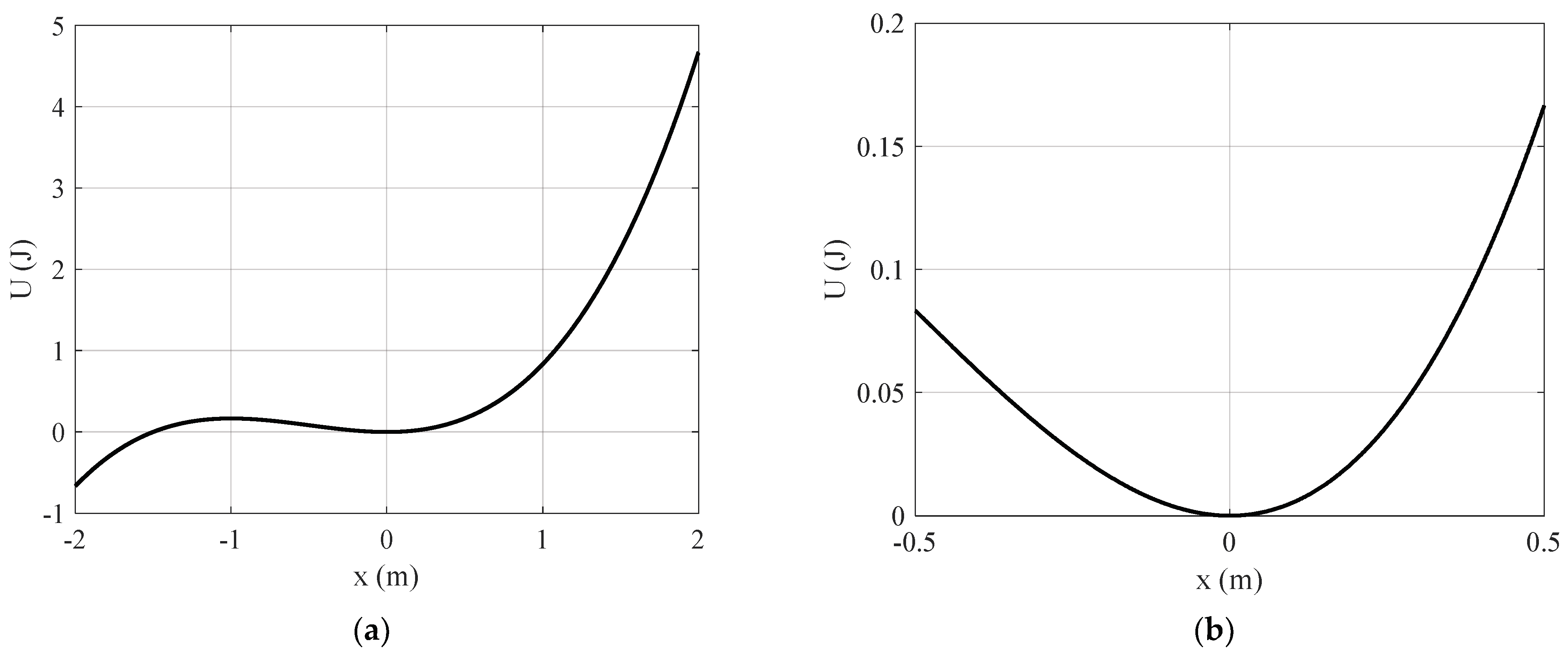
5. Vertical Oscillations under the Influence of Nonlinear Elastic Forces
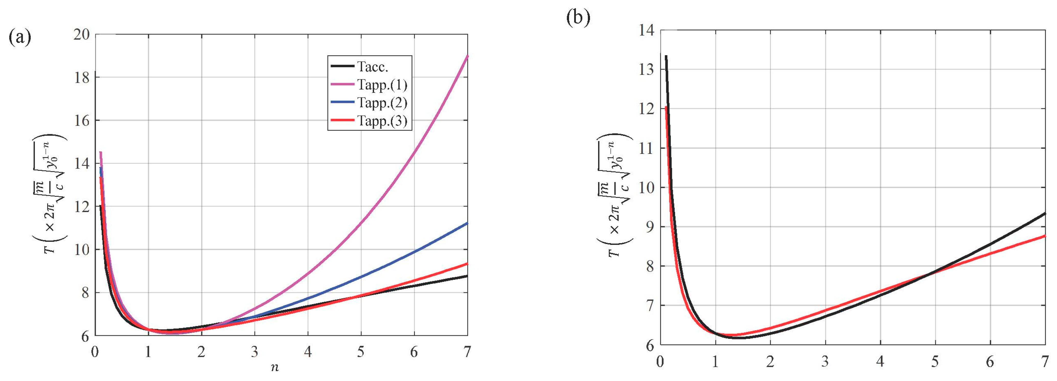
Another interesting case of nonlinear oscillator is the case of a vertical oscillation of an object with mass m at a constant gravitational field g combined with a nonlinear elastic force described by a power law equation F = c y n (where c   and   n are positive constants). The range of the object’s displacements is 0 y y 0 . At the moment t = 0 , it is assumed that y = 0 and d y d t = 0 . In addition, assuming that the positive direction is the weight’s direction, the differential equation of the motion is as in [18]:
m d 2 y d t 2 = w + F m d 2 y d t 2 = w c y n d 2 y d t 2 + c m y n g = 0
The oscillation’s period in this case is as in [18]:
T = 2 2 π m n + 1 y 0 1 n c Γ 1 + 1 2 n Γ n + 1 2 n
In Equation (21), Γ is the gamma function. For n = 1 , the result is the well-known equation for the harmonic motion’s period:
T = 2 π m c
An approximate equation that can be used instead of Equation (21) is based on calculating the ‘average stiffness’ [18]:
S ¯ = Δ F Δ y = c y 0 n y 0 = c y 0 n 1
In this case:
T = 2 π m S ¯   = 2 π m y 0 1 n c
Equation (24) is an acceptable solution for the range 0.7 n 2 [18]. The error compared to the accurate solution (21) is 1.965 % for n = 0.7 and 2.272 % for n = 2 . However, for other values, e.g., in the case that n = 0.6 , the error is significantly bigger (i.e., 6.21 % ). In this paper, the approach proposed by He [13] as per Equations (2) and (3), will be applied in the differential Equation (20). The basic goal is to find out whether He’s approach can provide a simple equation that can be applied for a bigger range of the exponential factor n compared to Equation (24). In the case of Equation (20), f y = c m y n g . Thus, using Equation (2),
ω a p p . 1 = d f y d y y 0 2 = n c m y n 1 y 0 2 = c m n 2 n 1 y 0 n 1
Thus, the oscillation’s period should be as follows:
T a p p . 1 = 2 π m c 2 n 1 n y 0 1 n
A second more accurate approach is to use Equation (3):
ω a p p . 2 = 1 3 d f y d y 0.3 y 0 + d f y d y 0.5 y 0 + d f y d y 0.7 y 0   ω a p p . 2 = c m n 1 3 0.3 n 1 + 0.5 n 1 + 0.7 n 1 y 0 n 1
and
T a p p . 2 = 2 π m c 3 n 0.3 n 1 + 0.5 n 1 + 0.7 n 1 y 0 1 n
Another idea is to use also a more ‘symmetric’ approach:
ω a p p . 3 = 1 3 d f y d y 0.25 y 0 + d f y d y 0.5 y 0 + d f y d y 0.75 y 0   ω a p p . 3 = c m n 1 3 0.25 n 1 + 0.5 n 1 + 0.75 n 1 y 0 n 1
and
T a p p . 3 = 2 π m c 3 n 0.25 n 1 + 0.5 n 1 + 0.75 n 1 y 0 1 n
The T = f n functions using the accurate solution (Equation (21)) and the approximate Equations (26), (28) and (30) are presented in Figure 2.

6. Discussion

Many methods for solving the cubic–quintic Duffing oscillator have been proposed in the literature. For example, Lai et al. [19] used the Newton–harmonic balancing method and Guo et al. applied an iterative homotopy harmonic balance method [20]. Khan et al. [21] used a method that combines the features of the homotopy concept with the variational approach. Ganji et al. applied He’s energy balance method and iteration perturbation method [22,23]. Akbarzade and Farshidianfar used the improved energy balance method and the global residue harmonic balance method [12]. Pirbodaghi et al. explored the homotopy analysis method and homotopy pade technique [24], while Razzak considered an analytical method that combines the homotopy perturbation method and a variational approach [25]. Accurate solutions of the cubic–quintic Duffing oscillator were recently derived by Zuniga [26], Zakeri [27] and Beléndez et al. [28,29]. However, the procedure is complex since it contains a set of complex nonlinear algebraic equations with Jacobian elliptic functions. Chowdhury et al. presented an analytical technique based on the harmonic balance method to determine higher-order approximate solutions [11]. In addition, recently, He provided the simplest approach for finding the angular frequency of the cubic–quintic Duffing oscillator [13]. Thus, since He’s approach is extremely simple, it is important to find whether it can be also used in other cases. In this paper, it was shown that it provides accurate results for the calculation of the oscillation’s period for many well-known cases. However, a significant question remains: why is He’s approach a reliable approach? The main idea behind He’s formulation is based on an engineering point of view. In fact, assume an oscillation of a point mass m described by the following equation:
m d 2 x d t 2 + F x = 0
In Equation (31), F(x) is the applied force on the mass. We can assume that the force is applied by a linear or a nonlinear spring. Under this perspective, the spring’s constant will be equal to the following:
k = d F x d x
In the case that the spring is linear, k=constant and the motion’s period is described by the trivial equation T = 2 π m / k . In this case, the period is independent from the oscillation’s amplitude. On the other hand, if the spring is not linear, then the oscillation’s period depends on the amplitude. However, we can assume an ‘equivalent linear problem’ (i.e., a harmonic case with the same period) for any given amplitude. Therefore, we need to determine the exact value of the spring constant of the abovementioned ‘equivalent linear problem’. For example, for the case of the simple pendulum, the force magnitude is provided below:
F θ = m g s i n θ
Thus, the ‘spring’s constant’ is as follows:
k = d F d x = m g l c o s θ
Using Equation (34), it can be concluded that k is bigger for small amplitudes. Thus, as the oscillation’s amplitude increases, the spring’s constant decreases and as a result the period increases. Hence, we need to find a ‘representative spring’s constant’ of a linear spring that approximately leads to correct results. The simplest idea is to consider that the spring’s constant of the equivalent linear problem is k e q . , which is given as follows:
  k e q . = m g l c o s ( θ 0 / 2 )
For a small range of amplitudes, this is an acceptable approach (for example, for the simple pendulum 0 θ π / 2 ). For other problems in which bigger amplitude’s range applies (e.g., the Duffing equation or the cubic–quintic Duffing oscillator), the method needs to be modified. However, in any case the main idea remains the same. We consider an ‘equivalent linear problem’ for a given amplitude. He’s approach is used to find the average value of the spring constant for x = 0.3 A, x = 0.5 A and x = 0.7 A, as in the following:
k e q . = 1 3 d F x d x 0.3 A + d F x d x 0.5 A + d F x d x 0.7 A
This approach provides good approximations for the case of the Duffing equation, the cubic–quintic Duffing oscillator and the Helmholtz nonlinear oscillator. For the general case of the vertical oscillations at a constant gravitational field under the influence of a nonlinear elastic force, the same equation can be applied; however, to achieve the biggest possible accuracy, the equivalent spring’s constant is as follows:
k e q . = 1 3 d F x d x 0.25 A + d F x d x 0.5 A + d F x d x 0.75 A
In conclusion, He’s approach can be summarized as follows: ‘in many cases of strong nonlinear oscillations we can consider an equivalent linear problem with the same period as the actual one’. Thus, the appropriate value of the spring constant should be determined in each case by following the methodology above (i.e., Equation (2), Equation (3) or Equation (29)).
Another interesting method for approximating the period of strong nonlinear oscillations was presented in [30]. The case that was considered is the following:
d 2 x   d t 2 1 + n = 1 b 2 n 1 x 2 n + m = 1 a 2 m 1 x 2 m 1 + n = 1 n b 2 n 1 x 2 n 1 d x d t 2 = 0
In the special case that b 2 n 1 = 0 , the differential equation above is simplified as follows:
d 2 x d t 2 + m = 1 a 2 m 1 x 2 m 1 = 0
This is the case examined in this paper. An example presented in [30] is the free vibration of a restrained uniform beam carrying an intermediate lumped mass (this case was first introduced by Hamdan and Shabaneh [31]):
d 2 x d t 2 + λ x + ε 1 x 2 d 2 x d t 2 + ε 1 x d x d t 2 + ε 2 x 4 d 2 x d t 2 + 2 ε 2 x 3 d x d t 2 + ε 3 x 3 + ε 4 x 5 = 0
The initial conditions that were chosen were x(0) = A, dx(0)/dt = 0. By introducing a new variable τ = ωt, it can be concluded as follows:
ω 2 d 2 x d t 2 + λ x + ε 1 ω 2 x 2 d 2 x d t 2 + ε 1 ω 2 x d x d t 2 + ε 2 ω 2 x 4 d 2 x d t 2 + 2 ε 2 ω 2 x 3 d x d t 2 + ε 3 x 3 + ε 4 x 5 = 0
A first approximation of the angular frequency is provided below:
ω = 8 λ + 6 A 2 ε 3 + 5 A 2 ε 4 8 + 4 A 2 ε 1 + 3 A 4 ε 2
In the special case that ε 1 = ε 2 = 0 and λ = ε 3 = ε 4 = 1 , it can be concluded as follows:
d 2 x d t 2 + x + x 3 + x 5 = 0
Thus,
ω = 8 + 6 A 2 + 5 A 4 8 = 1 + 3 4 A 2 + 5 8 A 4
This is a similar equation to the one provided by He’s approach:
ω H e = 1 3 d f x d x x = 0.3 A + d f x d x x = 0.5 A + d f x d x x = 0.7 A = 1 + 0.83 A 2 + 0.51783 A 4
The results are compared in Figure 3.
Similar results can be also found using the methods presented by El-Dib [32].

7. Conclusions

In this paper, it was shown that He’s formulation can be used in many different cases of nonlinear oscillators. Equation (2) can provide a perfect approximation for the case of the Duffing equation, the Helmholtz nonlinear oscillator and the simple pendulum. For the Duffing equation, He’s formulation provides accurate results even for very big oscillation amplitudes ( A ). In addition, for the simple pendulum the error is negligible for 0 θ π 2 . For the Helmholtz nonlinear oscillator, the error when using He’s approach is always smaller than 3%. Furthermore, He’s method is an accurate approach for the case of the vertical oscillations under the influence of nonlinear elastic forces. In this case, He’s approach is slightly modified to include a very wide range of elastic forces with exponents in the range 0.5 n 6.3 (Equations (29) and (30)).
The criterion for an acceptable approximation is that the error compared to the actual solution should be smaller than 4% as presented in He’s original paper [13]. Equations (21) and (30) provide similar results for 0.5 n 6.3 . In this case, the error is below 4%, as shown in Figure 4. Equation (26) is an acceptable solution for a small range of the exponent n. In particular, for 0.7 n 2.8 , the error is smaller than 4%. Equation (28) is also an acceptable solution for 0.7 n 3.7 (error smaller than 4%). It is also interesting to note that the error provided by the Equations (26), (28) and (30) is independent of the oscillation’s amplitude. These equations depend on the amplitude in the same way as the accurate solution (21) ( ~ y 0 1 n ). In conclusion, He’s formulation is a strong tool for finding approximate solutions regarding the period of nonlinear oscillations.

8. Future Work

An interesting question that may arise from the analysis above is whether He’s approach can be used for two or more degrees of freedom system. The reason is that in many cases, systems of two coupled second-order nonlinear differential equations are used to describe several physical phenomena [33]. For example, in plasma physics, the following system of equations applies [33]:
d 2 x d t 2 + m x 3 y = ε x 4 y
d 2 y d t 2 + p x 5 a x = 0
In Equations (46) and (47), p , m   and   a are constants and ε is a small parameter. Therefore, it would be interesting to examine whether He’s linearization method can be used in the abovementioned equations to provide a simplified method for solving the aforementioned system or other systems with many degrees of freedom.

Author Contributions

Conceptualization, S.V.K.; methodology, S.V.K. and A.M.; software, S.V.K. and G.C.; validation, S.V.K., G.C. and A.M.; formal analysis, S.V.K., G.C. and A.M.; investigation, S.V.K.; data curation, S.V.K. and A.M.; writing—original draft preparation, S.V.K.; writing—review and editing, S.V.K., G.C. and A.M. All authors have read and agreed to the published version of the manuscript.

Funding

This research received no external funding.

Institutional Review Board Statement

Not applicable.

Informed Consent Statement

Not applicable.

Data Availability Statement

Not applicable.

Conflicts of Interest

The authors declare no conflict of interest.

References

  1. Nayfeh, A.H.; Mook, D.T. Nonlinear Oscillations; Wiley: New York, NY, USA, 1979. [Google Scholar]
  2. Hagedorn, P. Non-Linear Oscillations; Clarendon: Oxford, UK, 1988. [Google Scholar]
  3. Cveticanin, L.; Kozmidis Luburic, U.; Mester, G. Periodic Motion in an excited and damped cubic nonlinear oscillator. Math. Probl. Eng. 2018, 2018, 3841926. [Google Scholar] [CrossRef]
  4. Big-Alabo, A. Approximate periodic solution and qualitative analysis of nonnatural oscillators based on the restoring force. Eng. Res. Express 2020, 2, 015029. [Google Scholar] [CrossRef]
  5. Big-Alabo, A. Approximate periodic solution for the large-amplitude oscillations of a simple pendulum. Int. J. Mech. Eng. Educ. 2019, 8, 335–350. [Google Scholar] [CrossRef]
  6. Kontomaris, S.V.; Malamou, A. Exploring the non-linear oscillation of a rigid sphere on an elastic half-space. Eur. J. Phys. 2021, 42, 025011. [Google Scholar] [CrossRef]
  7. Koruk, H. Modelling small and large displacements of a sphere on an elastic half-space exposed to a dynamic force. Eur. J. Phys. 2021, 42, 055006. [Google Scholar] [CrossRef]
  8. Stenflo, L.; Brodin, G. Temperature effects on large amplitude electron plasma oscillations. Phys. Plasmas 2016, 23, 074501. [Google Scholar] [CrossRef]
  9. Nayfeh, A.H. Perturbation Methods; Wiley: New York, NY, USA, 1973. [Google Scholar]
  10. He, J.H. Homotopy perturbation method with two expanding parameters. Indian J. Phys. 2014, 88, 193–196. [Google Scholar] [CrossRef]
  11. Chowdhury, M.S.H.; Hosen, M.A.; Ahmad, K.; Ali, M.Y.; Ismail, A.F. High-order approximate solutions of strongly nonlinear cubic-quintic Duffing oscillator based on the harmonic balance method. Results Phys. 2017, 7, 3962–3967. [Google Scholar] [CrossRef]
  12. Akbarzade, M.; Farshidianfar, A. Nonlinear transversely vibrating beams by the improved energy balance method and the global residue harmonic balance method. Appl. Math. Model. 2017, 45, 393–404. [Google Scholar] [CrossRef]
  13. He, J.H. The simplest approach to nonlinear oscillators. Results Phys. 2019, 15, 102546. [Google Scholar] [CrossRef]
  14. Almendral, J.A.; Sanjuán, M.A.F. Integrability and Symmetries of the Helmholtz oscillator with Friction. J. Phys. Math. Gen. 2003, 36, 695–710. [Google Scholar] [CrossRef]
  15. Almendral, J.A.; Seoane, J.; Sanjuán, M.A.F. The Nonlinear Dynamics of the Helmholtz Oscillator. Recent Res. Dev. Sound Vib. 2004, 2, 115–150. [Google Scholar]
  16. Kovacic, I.; Gatti, G. Helmholtz, Duffing and Helmholtz-Duffing Oscillators: Exact Steady-State Solutions. In IUTAM Symposium on Exploiting Nonlinear Dynamics for Engineering Systems; Kovacic, I., Lenci, S., Eds.; ENOLIDES 2018; IUTAM Bookseries; Springer: Cham, Switzerland, 2020; Volume 37. [Google Scholar]
  17. Kontomaris, S.V.; Malamou, A. Exploring oscillations with a nonlinear restoring force. Eur. J. Phys. 2022, 43, 015006. [Google Scholar] [CrossRef]
  18. Kontomaris, S.V.; Malamou, A. Nonlinear oscillations in a constant gravitational field. Phys. Scr. 2022, 97, 015202. [Google Scholar] [CrossRef]
  19. Lai, S.K.; Lim, C.W.; Wu, B.S.; Wang, C.; Zeng, Q.C.; He, X.F. Newton-harmonic balancing approach for accurate solutions to nonlinear cubic-quintic Duffing oscillators. Appl. Math. Model. 2008, 33, 852–866. [Google Scholar] [CrossRef]
  20. Guo, Z.; Leung, A.Y.T.; Yang, H.X. Iterative homotopy harmonic balancing approach for conservative oscillator with strong odd-nonlinearity. Appl. Math. Model. 2011, 35, 1717–1728. [Google Scholar] [CrossRef]
  21. Khan, Y.; Akbarzadeb, M.; Kargar, A. Coupling of homotopy and the variational approach for a conservative oscillator with strong odd-nonlinearity. Sci. Iran A 2012, 19, 417–422. [Google Scholar] [CrossRef]
  22. Ganji, D.D.; Gorji, M.; Soleimani, S.; Esmaeilpour, M. Solution of nonlinear cubicquintic duffing oscillators using He’s Energy Balance Method. J. Zhejiang Univ. Sci. A 2009, 10, 1263–1268. [Google Scholar] [CrossRef]
  23. Ganji, S.S.; Barari, A.; Karimpour, S.; Domairry, G. Motion of a rigid rod rocking back and forth and cubic-quintic duffing oscillators. J. Theor. Appl. Mech. 2012, 50, 215–229. [Google Scholar]
  24. Pirbodaghi, T.; Hoseini, S.H.; Ahmadian, M.T.; Farrahi, G.H. Duffing equations with cubic and quintic nonlinearities. Comput. Math. Appl. 2009, 57, 500–506. [Google Scholar] [CrossRef]
  25. Razzak, M.A. An analytical approximate technique for solving cubic–quintic Duffing oscillator. Alex. Eng. J. 2016, 55, 2959–2965. [Google Scholar] [CrossRef]
  26. Zuniga, A.E. Exact solution of the cubic–quintic Duffing oscillator. Appl. Math. Model. 2013, 37, 2574–2579. [Google Scholar] [CrossRef]
  27. Zakeri, G.A.; Yomba, E. Exact solutions of a generalized autonomous Duffing-type equation. Appl. Math. Model. 2015, 39, 4607–4616. [Google Scholar] [CrossRef]
  28. Beléndez, A.; Beléndez, T.; Martínez, F.J.; Pascual, C.; Alvarez, M.L.; Arribas, E. Exact solution for the unforced Duffing oscillator with cubic and quintic nonlinearities. Nonlinear. Dyn. 2016, 86, 1687–1700. [Google Scholar] [CrossRef]
  29. Beléndez, A.; Arribas, E.; Beléndez, T.; Pascual, C.; Gimeno, E.; Álvarez, M.L. Closed form exact solutions for the unforced quintic nonlinear oscillator. Adv. Math. Phys. 2017, 14, 7396063. [Google Scholar] [CrossRef]
  30. Cveticanin, L.; Ismail, G.M. Higher-order approximate periodic solution for the oscillator with strong nonlinearity of polynomial type. Eur. Phys. J. Plus 2019, 134, 266. [Google Scholar] [CrossRef]
  31. Hamdan, M.N.; Shabaneh, H.J. On the large amplitude free vibrations of a restrained uniform beam carrying an intermediate lumped mass. J. Sound Vib. 1997, 199, 711–736. [Google Scholar] [CrossRef]
  32. El-Dib, Y.O. Insightful and comprehensive formularization of frequency–amplitude formula for strong or singular nonlinear oscillators. J. Low Freq. Noise Vib. Act. Control. 2023, 42, 89–109. [Google Scholar] [CrossRef]
  33. Cveticanin, L. Analytic solution of the system of two coupled differential equations with the fifth-order non-linearity. Phys. A Stat. Mech. Its Appl. 2003, 317, 83–94. [Google Scholar] [CrossRef]
Figure 1. The U = f x graph (a) for 2   m x 2   m and (b) for 0.5   m x 0.5   m . The graphs were plotted using Equation (11).
J 06 00010 g001
Figure 2. (a) The T = f n functions using the accurate solution (Equation (21)) and the approximate Equations (26), (28) and (30). (b) The T = f n functions using Equation (21) (black curve) and (30) (red curve). Equation (30) is the more accurate approach in this case.
J 06 00010 g002
Figure 3. The angular velocity for the case of Equation (43) when using the Cveticanin approach (blue curve) [30] and He’s approach (red curve) [13].
J 06 00010 g003
Figure 4. The error in period’s calculation if using Equation (30) with respect to the exponent n of the power law elastic force.
J 06 00010 g004
Table 1. Accurate and approximate solutions for Duffing equation for m = 1   kg , c 1 = 1   kgs 2 and c 2 = 1   kgm 2 s 2 .
A (m)T(s) (Using Equation (7))T (s) (Using Equation (9))Error (%)
0.16.25986.25971.5975 × 10 3
0.36.08186.08138.2213 × 10 3
0.55.76895.76585.3736 × 10 2
14.76804.74963.8591 × 10 1
23.17973.14161.1982
51.44191.41381.9488
100.73620.720732.1013
1000.074160.072542.1845
10000.0074160.0072552.1710
Table 2. Accurate and approximate solutions for oscillators with a quadratic restoring force for m = 1   kg , c 1 = 1   kgs 2 and c 2 = 1   kgm 1 s 2 .
A (m)T(s) (Using Equation (13))T (s) (Using Equation (14))Error (%)
0.056.15406.13180.3607
0.106.03265.99080.6929
0.155.91835.85911.0003
0.205.81025.73571.2822
0.255.70805.61991.5434
0.305.61115.51071.7893
0.355.51895.40772.0149
0.405.43125.31032.2260
0.455.34765.21792.4254
0.505.26785.13022.6121
Disclaimer/Publisher’s Note: The statements, opinions and data contained in all publications are solely those of the individual author(s) and contributor(s) and not of MDPI and/or the editor(s). MDPI and/or the editor(s) disclaim responsibility for any injury to people or property resulting from any ideas, methods, instructions or products referred to in the content.

