Ionic Imbalances and Coupling in Synchronization of Responses in Neurons

Abstract

Most neurodegenerative diseases (NDD) are a result of changes in the chemical composition of neurons. For example, Alzheimer’s disease (AD) is the product of Aβ peptide deposition which results in changes in the ion concentration. These changes in ion concentration affect the responses of the neuron to stimuli and often result in inducing excessive excitation or inhibition. This paper investigates the dynamics of a single neuron as ion changes occur. These changes are incorporated using the Nernst equation. Within the central and peripheral nervous system, signals and hence rhythms, are propagated through the coupling of the neurons. It was found that under certain conditions the coupling strength between two neurons could mitigate changes in ion concentration. By defining the state of perfect synchrony, it was shown that the effect of ion imbalance in coupled neurons was reduced while in uncoupled neurons these changes had a more significant impact on the neuronal behavior.

1. Introduction

In the nervous system, neuronal cells (neurons) communicate with each other via electrical events. These neurophysiological electrical events are called action potentials. Action potentials within a neuron are generated because of both an external stimulus and chemical diffusion of ions [1]. This has been extensively studied in different models [2,3,4,5,6,7]. The common feature in all these studies is the close relationship between the ions within a neuron and the external stimulus. Neurons have three essential components: the soma, the axon, and the dendrites (see Figure 1). The external stimulus, when applied to a neuron, results in changes within the neuron which generate an action potential. This action potential, which is transmitted from one neuron to another, is characterized by the magnitude of the spikes and the interval between the spikes. These characters follow a principle in neurophysiology called all-or-none. All-or-none is a principle whereby the strength by which an excitable cell response to any stimulus is not dependent on the strength of that stimulus, given that the stimulus is of an adequate strength [8].

Although the effects of chemical imbalances on neuronal signals have been studied [9,10], these have not included the effects of chemical imbalances over a network of neurons. In coupled neurons, it is important to understand the manner in which the neurons work synchronously and the nature of the resultant spike train as an output. A chemical imbalance in one neuron changes the dynamics of other neurons connected to it. As a result, there are two kinds of effects in a chain of neurons, one is the loss of synchronicity and the other is a change in the inter-spike interval and the magnitude of the spikes. A change in the chemical balance results in a change in the action potential.

Synchronization is the mechanism that maintains vital rhythms, like that of respiration. The firing of many neurons, if they are synchronized, gives rise to measurable fluctuations of the electroencephalographical (EEG) signal. Synchronization is also responsible for the generation of pathological tremors and plays a significant role in several neurological diseases, like epilepsy [11]. Spectral analysis of EEG signal shows that neurons can oscillate synchronously in various frequency bands, from less than 2 Hz to greater than 60 Hz [12]. Numerical experiments suggest that when two sets of equations are coupled, their solutions seem to synchronize. Experimental findings of synchronization in excitable tissue provide these results. However, mathematical models for these systems are typically very complicated. For couplings between oscillators, two types of couplings can be found in the real nervous system: a) the chemical synapse and b) the electrical synapse. Chemical synapses contain nonlinear couplings, whereas electrical synapses have linear membrane potentials.

In recent years, several studies have been performed investigating the various effects of coupling and synchronization in neuronal systems. These works included studies of the effects of the spike plasticity on synchronization [13], synchronization in clustered networks [14], synchronization in the different type of networks [15,16], and the dynamics of coupled neurons [17,18]. Studies have been carried out investigating responses to different classes of stimuli, e.g., visual [19], odorous [20], tactile [21] or synchronization of neurons, as reported by Stern et al. [22]. However, the majority of these studies concentrated on either the theoretical or the practical concepts of synchrony and most of them separated computational applications from the clinical point in their investigations.

In this paper, electrolyte imbalances were investigated from a coupling and synchronization phenomenon point of view. The remainder of this manuscript is organized in the following way. Section 2 describes voltage-gated ion channels. Section 3 describes membrane potential dynamics. Simulation and results are presented in Section 4. Finally, the results of the experiments and simulation are discussed in Section 5.

2. Voltage-Gated Ion Channels

The schematic neuron, shown in Figure 1, is an electrically excitable cell which is found in the nervous system. Neurons have three essential functions: (a) to receive signals, (b) to integrate incoming signals, and (c) to transfer signals to target cells, which can be other neurons, muscles, or glands. In a neuron, signals are generated by a variety of membrane-spanning ion channels that allow ions, mainly sodium (Na⁺), potassium (K⁺), and chloride (Cl⁻), to move in and out of the cell. These ion channels control the flow of ions by opening and closing in response to voltage changes. The voltage changes are a result of both external stimuli and internally generated signals [8]. The electrical signals of relevance to the nervous system are the difference in electrical potential between the interior of a neuron and the enclosing extracellular medium.

Under resting conditions the cell is said to be polarized. Ion pumps located in the cell membrane maintain concentration gradients that support the membrane’s potential difference. Sodium is much more concentrated outside a neuron than inside and the concentration of potassium is significantly higher inside the neuron than in the extracellular medium. Therefore, ions flow into and out of a cell due to concentration gradients as well as voltage. The process by which positively charged ions flow out of the cell and negatively charged ions flow into the cell through open channels creates a current. This current makes the membrane potential more negative and this process is called hyperpolarization. Current flowing into the cell changes the membrane potential to less negative or even positive values and this process is called depolarization (see Figure 2).

By depolarizing a neuron and bringing the membrane potential above a threshold level, a positive feedback process is initiated, and the firing neuron, as shown in Figure 2, generates a spike or action potential. The generation of the action potential is very dependent on the recent history of cell firing. So that, a few milliseconds after a spike, it may be impossible to initiate a next action potential; this is the refractory period. Action potentials then regenerate actively along axon processes. Those can travel rapidly over long distances without any attenuation. According to the given description, the role of ions in neural communication is critical; any imbalances can have harmful effects on the nervous system. Section 2.1 describes ionic imbalances in the nervous system. Biologists such as Alan Hodgkin and Andrew Huxley [23] have mathematically modelled the electrical process of the nervous system with a set of differential equations, as discussed in Section 3.

2.1. Ionic Imbalances

Ionic imbalances strongly affect neuronal activity and are implicated in cell death in both the central and peripheral nervous systems and in other tissues like myocardium or skeletal muscles. An excess of sodium ion concentration is known as hypernatremia and the converse is called hyponatremia. Similarly, excessive potassium ion concentration is known as hyperkalemia, and the opposite is defined as hypokalemia. An imbalance in sodium and potassium, especially hyponatremia and hypokalemia, are a common challenge in clinical practice [24]. These are common electrolyte disorders in the context of central nervous system (CNS) disease [25]. Ionic imbalances have a broad range of neurological effects in disorders such as epileptiform seizures, muscle rigidity, and tremor. Imbalances depress the central nervous system and produce lethargy that progresses to coma. Permanent brain damage may result from severe imbalances.

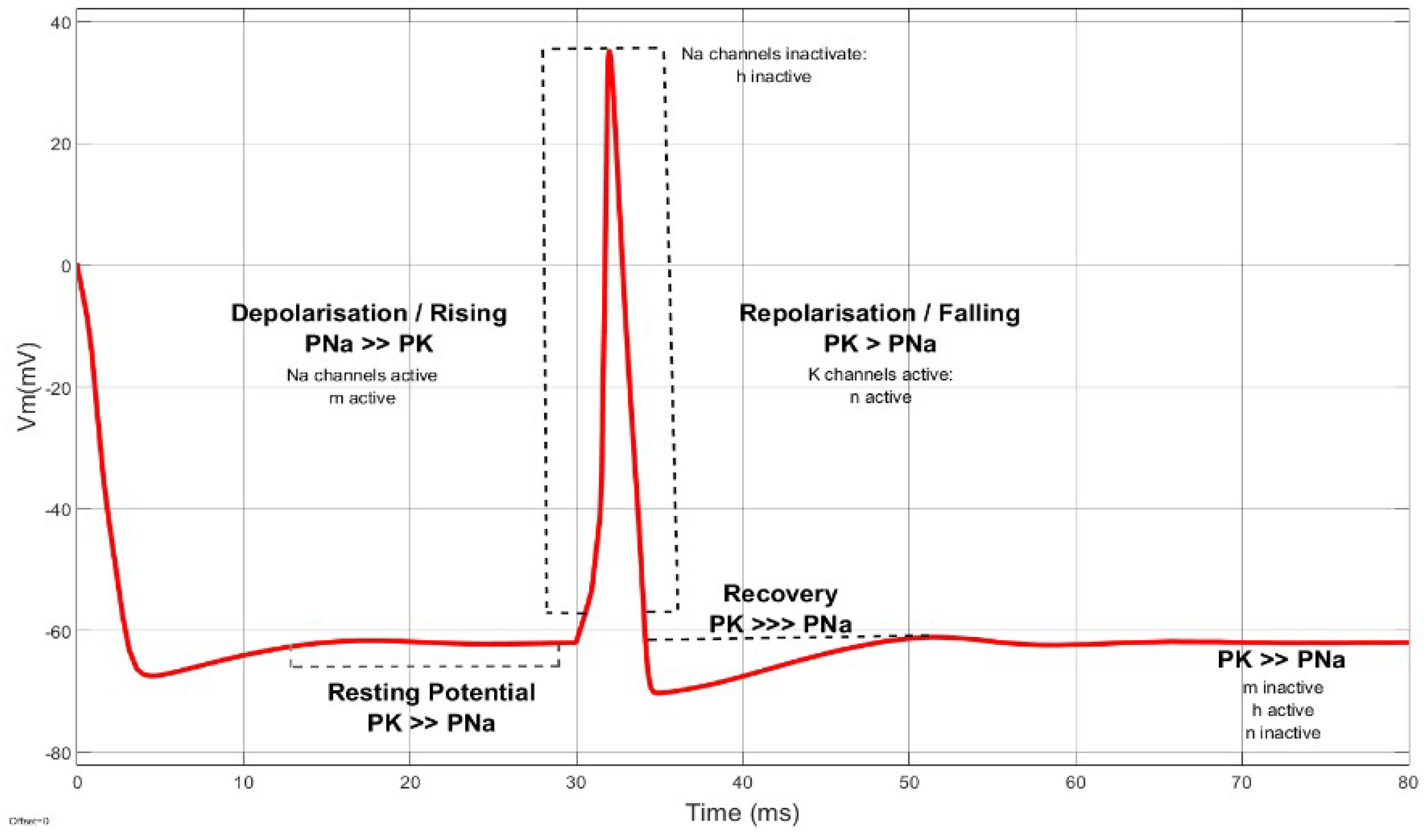
3. Membrane Potential Dynamics

A number of different types of neurons have been studied and modelled, for example, squid axons [5], frog [4], dog [6], rabbit [2], cat [3], and the Purkinje cell [7]. The common feature of these models is that they are based on the membrane potentials of the cells and the ion channel dynamics. In general, these models take the form:

$$C_m\frac{dV}{dt}=I-f\left(\theta ,\overline{V}\right)$$

(1)

where C_m is the membrane capacitance, I is the current, V is the membrane potential in mV, and t is time. The various forms of the mathematical models are based on the structure and form of $f\left(\theta ,\overline{V}\right)$. This term is a function of (a) the probabilities of the opening and closing of an ion channel, (b) the conductivity of the ion channel, and (c) the potential difference between the membrane and the ion channel (given by V). In general, $f\left(\theta ,\overline{V}\right)$ is an algebraic sum of the currents associated with the various ion channels, and, thus, a specific ion, i, would take the form:

$$f_i\left({\theta }_i,V_i\right)=g_i\left(V-\overline{V_i}\right)$$

(2)

$$and f\left(\theta ,\overline{V}\right)=\sum _i{f}_i={\displaystyle \sum }_i{g}_i(V-\overline{V_i})$$

(3)

where the variable $g_i$ is a function of the probabilities of the opening and closing of channels, and the conductance of that particular channel. The membrane potential dynamics activate and deactivate the channels (see Section 2). If the neuron dynamics are restricted to sodium and potassium channels, these become:

$$\frac{dn}{dt}={\alpha }_n\left(V\right)\left(1-n\right)-{\beta }_n\left(V\right)n$$

(4)

$$\frac{dm}{dt}={\alpha }_m\left(V\right)\left(1-m\right)-{\beta }_m\left(V\right)m$$

(5)

$$\frac{dh}{dt}={\alpha }_h\left(V\right)\left(1-h\right)-{\beta }_h\left(V\right)h$$

(6)

where n, m, and h are representations of the fractions of the open and closed channels for the different ions. Thus, the membrane potential based model takes the form:

$$\frac{dV}{dt}=I_{inj}+\sum _{i=1}^N{g}_i{\psi }_i\left(y_i\right)\left(V-V_i\right)$$

(7)

where $\psi$ are given by n, m, and h. This model describes the time behavior of the intracellular membrane potential and the currents through the channels. It is possible to explain observed phenomena accurately, and the change of voltages and currents on the nerve cell membrane can be analyzed quantitatively [26]. For the channels under consideration, the parameters given in Equations (4)–(6) are defined as follows:

$${\mathsf{\alpha }}_{\mathrm{n}}\left(\mathrm{V}\right)=\frac{0.01\left(\mathrm{V}+55\right)}{1-\exp \left[-\frac{\mathrm{V}+55}{10}\right]}$$

(8)

$${\mathsf{\beta }}_{\mathrm{n}}\left(\mathrm{V}\right)=1.125\exp \left[-\frac{\mathrm{V}+65}{80}\right]$$

(9)

$${\mathsf{\alpha }}_{\mathrm{m}}\left(\mathrm{V}\right)=\frac{0.01\left(\mathrm{V}+40\right)}{1-\exp \left[-\left(\mathrm{V}+40\right)/10\right]}$$

(10)

$${\mathsf{\beta }}_{\mathrm{m}}\left(\mathrm{V}\right)=4\exp \left[-\left(\mathrm{V}+65\right)/18\right]$$

(11)

$${\mathsf{\alpha }}_{\mathrm{h}}\left(\mathrm{V}\right)=0.07\exp \left[-\left(\mathrm{V}+65\right)/20\right]$$

(12)

$${\mathsf{\beta }}_{\mathrm{h}}\left(\mathrm{V}\right)=\frac{1}{1+\exp \left[-\left(\mathrm{V}+35\right)/10\right]}$$

(13)

Based on the relationships between permeability, and conductance within the neuron [5], Equation (2) can be obtained for the current generated within a particular ion channel. So, the three states, for sodium, potassium, and leakage are given by the following algebraic equations:

$$I_{Na}=g_{Na}{m}^{3}h\left(V-V_{Na}\right)$$

(14)

$$I_K=g_K{n}^4\left(V-V_K\right)$$

(15)

$$I_L=g_L\left(V-V_L\right)$$

(16)

In these equations, V is the trans-membrane potential. I_inj is the sum of external and synaptic currents. I_Na is the current in the sodium channel and I_k in the potassium. I_L is the leakage current. The gating variables indicating activation and inactivation of the sodium ion current are 0 ≤ m ≤ 1 and 0 ≤ h ≤ 1, respectively. The gating variable showing activation of potassium ion current is 0 ≤ n ≤ 1. The membrane capacitance is $C_m$ = 1.0 μF/cm². V_Na and V_K are the equilibrium potentials for the sodium and potassium ions. For channels that conduct a single type of ion, the equilibrium potential can be easily determined. This equilibrium potential point has a direct relation with the each ion and can give via the Nernst equation. This equation can be used to predict the membrane voltage of a cell in which the plasma membrane is permeable to one ion only.

$$V_{ion}=\frac{\mathrm{R}T}{z\mathrm{F}}\ln \frac{{\left[C\right]}_{out}}{{\left[C\right]}_{in}}$$

(17)

In Equation (17), V is the potential for both sodium and potassium measured in volts. R is the universal gas constant, which is 8.314 J·K⁻¹·mol⁻¹. T is the temperature measured in degrees Kelvin, K = 273.16 + °C. F is the Faraday constant, which is 96,485·mol⁻¹ or J·V⁻¹·mol⁻¹. z is the valence of the ion, i.e., sodium is z = 1 and potassium is z = −1. The parameters [C]_in and [C]_out are concentrations of the ions inside and outside the cell, respectively. In equilibrium, the Nernst potentials of Equation (17) of all the diffusing ionic species are the same and equal to the membrane potential.

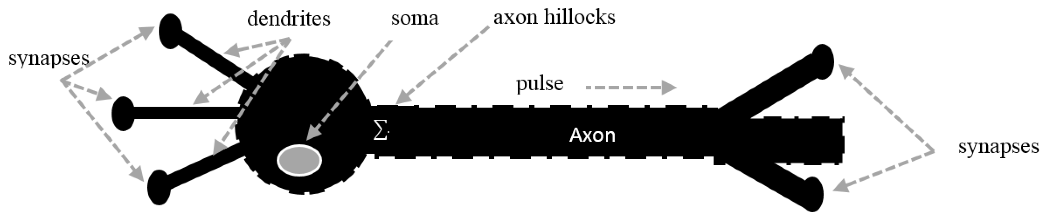
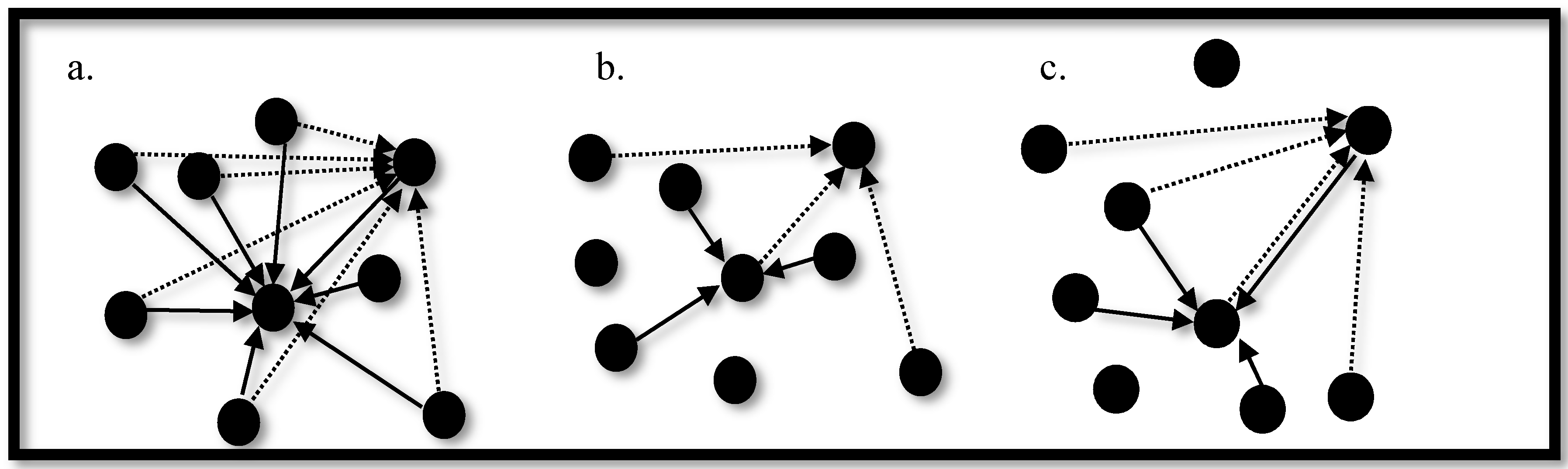
3.1. Generalized Form of Neurons

In this section, a generalized form of a neuron is presented for the N channels and m gates. The reason is to rewrite a mathematically pure form. First, consider Equations (1) and (4)–(7). In these equations the part $g_i\left(V-V_i\right)$ is common for all channels and, when $i=0,$ we get a leakage current. For ion currents the activation and deactivation gates can be rewritten as follows:

$$m^{3}h=u_{Na}\left(m,h\right)={\gamma }_m^3\left(v\right){\gamma }_h\left(v\right)={\psi }_{Na}\left(y\right)$$

(18)

$$n^4=u_K\left(n\right)={\gamma }_n^4\left(v\right)={\psi }_K\left(y\right)$$

(19)

These equations calculate the probability of the opening/closing channel for sodium and potassium, respectively. Using this information, the generalized form of a neuron with N channels and m ionic gates is in the form:

$$\frac{dV}{dt}=\mathrm{I}+g_0\left(V-V_0\right)+\sum _{i=1}^N{g}_i{\psi }_i\left(y\right)\left(V-V_i\right)$$

(20)

where each part of $g_i{\psi }_i\left(y\right)\left(V-V_i\right)$ models a specific ion channel. The channel status is denoted by variable $y$. In the original Hodgkin–Huxley model, with two channels and three gates, the variable y = ($y_1$,$y_2,y_3$) and the functions of $\psi$ are ${\psi }_1=y_1^3{y}_3$ and ${\psi }_2=y_2^4$. These functions are defined as probabilities and are in the range [0–1]. For this model, $y_1=n,$ $y_2=m,$ and $y_3=h$.

From Equation (4) we get:

$$\frac{dn}{dt}={\alpha }_n\left(v\right)\left(1-n\right)-{\beta }_n\left(v\right)n={\alpha }_n\left(v\right)-n\left({\alpha }_n\left(v\right)+{\beta }_n\left(v\right)\right)$$

(21)

By dividing and multiplying the right side of Equation (21) with ${\alpha }_n\left(v\right)+{\beta }_n\left(v\right)$, we get:

$$\left(\frac{{\alpha }_n\left(v\right)}{{\alpha }_n\left(v\right)+{\beta }_n\left(v\right)}-n\right)\left({\alpha }_n\left(v\right)+{\beta }_n\left(v\right)\right)$$

(22)

If $y_i=n,{\sigma }_i\left(v\right)=\frac{{\alpha }_n\left(v\right)}{{\alpha }_n\left(v\right)+{\beta }_n\left(v\right)}$ and ${\mathsf{\delta }}_i\left(v\right)={\alpha }_n\left(v\right)+{\beta }_n\left(v\right),$ Equation (21) is rewritten as follows:

$$\frac{d{y}_i}{dt}=({\sigma }_i\left(v\right)-y_i){\delta }_i\left(v\right)$$

(23)

Finally, the generalized form of a neuron model with N channels and m gates can be rewritten as follows [27]:

$$\begin{gathered} \{\begin{array}{ll}\frac{dV}{dt}=\mathrm{I}+g_0\left(V-V_0\right)+{\displaystyle \sum _{i=1}^N}{g}_i{\psi }_i\left(y_i\right)\left(V-V_i\right)=L\left(v,y,p\right),& {\psi }_i:{\mathfrak{K}}^m\to \mathfrak{K}\\ \frac{d{y}_j}{dt}=\mathrm{T}({\mathsf{\sigma }}_j\left(v\right)-y_j){\mathsf{\delta }}_j\left(v\right)=K_j\left(v,y_j,T\right),& {\mathsf{\delta }}_j,{\sigma }_j:\mathfrak{K}\to \mathfrak{K} \\ {\mathsf{\delta }}_j,{\sigma }_j\left(v\right)\ne 0\end{array} \end{gathered}$$

(24)

where the parameters p = ($g_0,\dots ,g_N,V_0,\dots ,V_N,I$) and the constant T > 0 are dependent on temperature. The dynamic of each gate variable $y_j$ depends only on itself, the voltage, $V,$ by smooth function ${\sigma }_i$ and the diagonal matrix ${\delta }_i\left(v\right)$ for all values of V. Each of the terms of $g_i {\psi }_i\left(y_j\right)\left(V-V_i\right)$ in Equation (24), with a constant $g_i,$ refer to an ionic channel. This adjusts the voltage, $V,$ across the nerve cell’s membrane and makes the dynamics of the $i$th channel. So, the generalized form of the neuron model in Equation (24) represents N channels and m gates where N and m are not necessarily equal. The model in Equation (24) is suitable for shaping a single neuron’s behavior. However, when two or more neurons in a network work together they are coupled by synapse spaces, which are not referred to in Equation (24). The missing link here is the coupling phenomenon, which is discussed in the next section.

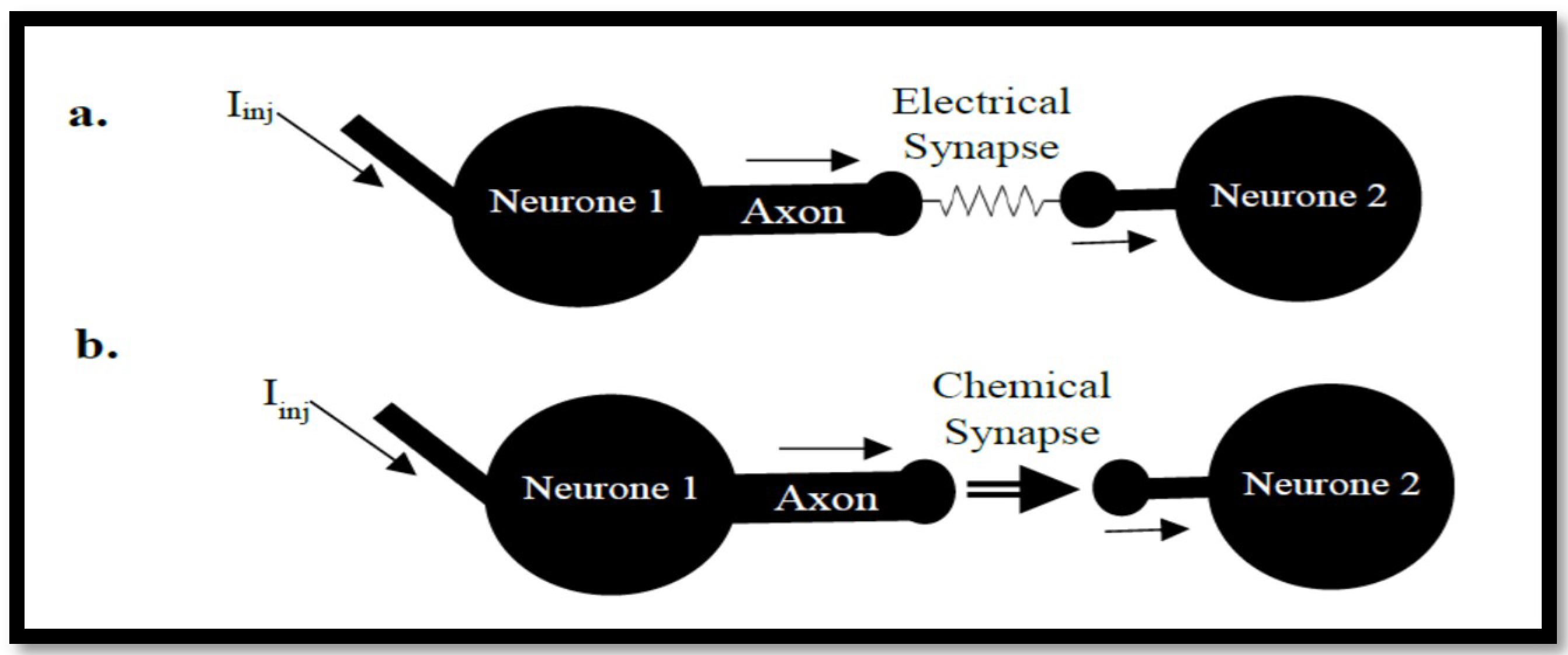
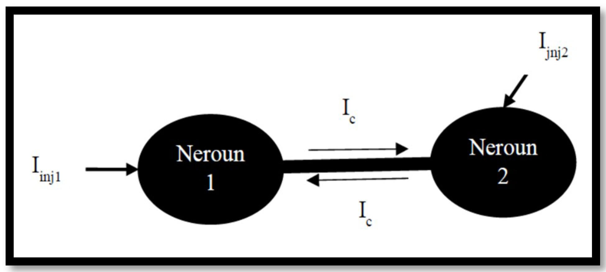
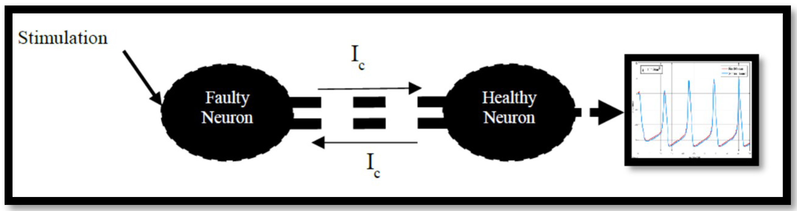
3.2. Coupled Type Equations

Coupling in the neurons is done via synapses. A live neuron is an oscillator that can be coupled with the chain of neurons (see Figure 3). A synapse can be explained as a site where a neuron makes a communicating connection with the next neuron. On one side of the synapse is a neuron that transmits the signal via the axon terminal, which is called the presynaptic cell and on the other side is another neuron, or a surface of an effector, that receives the signal and is called the postsynaptic cell. In nervous systems, there are three general types of synaptic connections among neurons.

All kinds of synapses are shown in Figure 4. Electrical connections are also known as gap junctions. Other forms of synapses are two types of chemical connections, excitatory and inhibitory. This study constructed neuron pair models by electrical synapse. The electrical connections are usually axon-to-axon, or dendrite-to-dendrite and are shaped by channel proteins that span the membranes of both connected neurons. Electrical coupling is ubiquitous in the brain, in particular among the dendritic trees of inhibitory interneurons. This kind of direct non-synaptic interaction allows for electrical communication between neurons. All models with electrical coupling necessarily involve a single neuron model that can represent the shape of an action potential.

The experiments in this study show that when two equations of neuron models are coupled, their solutions seem to synchronize. This paper investigates two of the same action potential equations, coupled only with the electrical potential of each neuron.

Choosing a large enough coupling strength forces the neuron to have the same behavior regardless of the initial condition. Mathematical models for such systems are frequently very complicated. Consider a pair of equations for a neuron model with partial coupling and coupling constants, p₁ and p₂ ≥ 0, using Equation (24) [28]:

$$(HHC)\{\begin{array}{ll}\frac{dv}{dt}=-p_1\left(v-u\right)+L\left(v,y,p\right)& \frac{du}{dt}=-p_2\left(u-v\right)+L\left(v,y,p\right)\\ \frac{d{y}_j}{dt}=K_j\left(v,y_j,T\right)& \frac{d{z}_j}{dt}=K_j\left(v,y_j,T\right)\end{array}$$

(25)

Later, we will show that for sufficiently large p₁ and p₂ the solutions of the above equation always synchronize. Synchronicity is tackled in Section 3.3.

3.3. Synchronization in Coupled Neurons

In this section, the mathematical background for the synchronization of coupled neurons is presented. Synchronization is a phenomenon that can be seen in two or more coupled neurons. It is achieved by an adjustment of rhythms and their oscillations. Synchronization is one of the important features of nonlinear systems. Nonlinear systems can show behaviors that are impossible in linear systems [29]. Synchronization analysis is a principle to discover interactions between nonlinear oscillators [29]. In the synchronization between two neurons, their action potentials have relatively equal frequencies. This closeness relies on the strength of the coupling. Therefore, spike synchronization is crucially dependent on the inter spike frequency. The general case of two coupled neurons can be characterized as follows:

$${\dot{v}}_1=L\left(v_1,v_2,{\lambda }_1\right) {\dot{v}}_2=L\left(v_2,v_1,{\lambda }_2\right),v_1,v_2\in R^n$$

(26)

where ${\lambda }_i$ = (g₀, …, g_N, V₀, …, V_N, I), which are dependent on parameter $\lambda$. Perfect synchronization happens when $v_1\left(t\right)=v_2\left(t\right)$ for all times t (Labouriau & Rodrigues, 2003). This coupled system is symmetric if ${\lambda }_1={\lambda }_2$ and asymmetric if ${\lambda }_1\ne {\lambda }_2$. Perfect synchrony usually does not happen in asymmetric systems. Consider Equation (25), in this equation, when p₁ = p₂, the coupled system is symmetric [28]. The solution of Equation (26) is synchronized if $v_1\left(t\right)$ and $v_2\left(t\right)$ remain close to each other in the next periods of action potentials. This means that, if there is a constant $\gamma >0$ and a continuous function like $f\left(t\right)\ge 0$ defined for $t\ge t_0$ in which $\underset{t\to \infty }{\lim }f\left(t\right)=0$ in a way that for all $t\ge t_0$, the following are true [28]:

$$\left|\Delta v\left(t\right)\right|\le \gamma ·f\left(t\right)·\left|\Delta \lambda \right|$$

(27)

After a short interaction between the two neurons the synchronicity between them becomes higher. Generally, for the symmetric case, there is an exponential decay to perfect synchronization [28].

3.4. The Region of Synchronicity

Coupled neurons often possess symmetries; these behaviors are important for understanding dynamic effects in systems. The simplest symmetric system contains two coupled neurons. Figure 5 presents two coupled neurons.

When the input current I_inj1 is applied it integrates into the axon hillock of the first neuron. These synaptic inputs cause the membrane to depolarize; that is, they cause the membrane potential to rise. If this polarization causes the membrane potential to rise to the threshold, an action potential V₁ can be raised. When an action potential is triggered, it abruptly generates a dendritic current that flows through the axon I_c in the output of the first neuron. By considering Equations (1)–(3) and Equations (14)–(16), the output of the first neuron for original Hodgkin–Huxley model is:

$$\dot{V_1}=\frac{1}{C_m}\left[I_{inj2}-I_{Na}-I_K-I_L+I_c\right]\to C_m\dot{V_1}=I_{inj1}-I_{Na}-I_K-I_L+I_c$$

(28)

Similarly, for the second neuron, the output is:

$$\dot{V_2}=\frac{1}{C_m}\left[I_{inj2}-I_{Na}-I_K-I_L+I_c\right]\to C_m\dot{V_2}=I_{inj2}-I_{Na}-I_K-I_L+I_c$$

(29)

In entirely normal conditions, if neuron number two is stimulated only by neuron number one and does not get any other stimuli from other neurons, the outputs of Equations (28) and (29) should be equal.

$$I_c\ge \frac{I_{inj1}}{2}$$

(30)

Equation (30) means to make synchronization between two neurons the minimum condition and should be respected.

4. Simulation and Results

4.1. Ion Imbalances in Neural Networks

Two sets of experiments were carried out. The first set of experiments compared the behavior of the output of action potentials in the hyper/hyponatremia and hyper/hypokalemia conditions for a single neuron and the second set of experiments was done for coupled neurons. All the experiments were carried out at simulation time of 1000.0 s. The injected current varied from 0 nA, between 0.0 to 50.0 s, and between 51.0 to 1000.0 s for 10 nA. The reason for considering two different injection currents was to have the behavior of the system under both stimulation and non-stimulation. A key element of this study was to investigate the effects of changing ion concentrations. These concentrations affected both the currents and the voltages in the model. The effects of the concentration of the ions are given by the Nernst equation [30], Equation (17), and rewritten as follow:

$$V_{N{a}^{+}}= \frac{\mathrm{R}T}{z\mathrm{F}}\ln \frac{{\left[N{a}^{+}\right]}_o}{{\left[N{a}^{+}\right]}_i}$$

(31)

$$V_{K^{+}}= \frac{\mathrm{R}T}{z\mathrm{F}}\ln \frac{{\left[K^{+}\right]}_o}{{\left[K^{+}\right]}_i}$$

(32)

where [K⁺]_o is the extracellular concentration of potassium, [K⁺]_i is the intracellular concentration of potassium, [Na⁺]_i is the intracellular concentration of sodium, and [Na⁺]_o is the extracellular concentration of sodium. Therefore, increasing/decreasing the V, has a direct relation with increasing/decreasing ${\left[N{a}^{+}\right]}_o$ and ${\left[K^{+}\right]}_o$. Hypernatremia (hyponatremia) and hyperkalemia (hypokalemia) are high (low) serum sodium and potassium levels, respectively, so changing the potential of the sodium and potassium means changing the ${\left[N{a}^{+}\right]}_o$ and ${\left[K^{+}\right]}_o$. As in Equations (31) and (32), ${\left[N{a}^{+}\right]}_o$ and ${\left[K^{+}\right]}_o$ have a direct relation to $V_{N{a}^{+}}$ and $V_{K^{+}}$. For this reason, in the experiments, by increasing or decreasing $V_{ion},$ the specific ion imbalances were simulated.

Figure 6 shows the responses of the neuron for the nominal set of values. It can be seen that the response is a series of spikes, which have two characteristics. One is the magnitude of the spike and the other is the time between spikes, known as an inter-spike interval. This response was taken to be the ideal response and all comparisons are made in relation to this response. The comparison was carried out for four different electrolyte diseases, i.e., hypernatremia, hyponatremia, hyperkaliemia, and hypokalemia and combinations thereof.

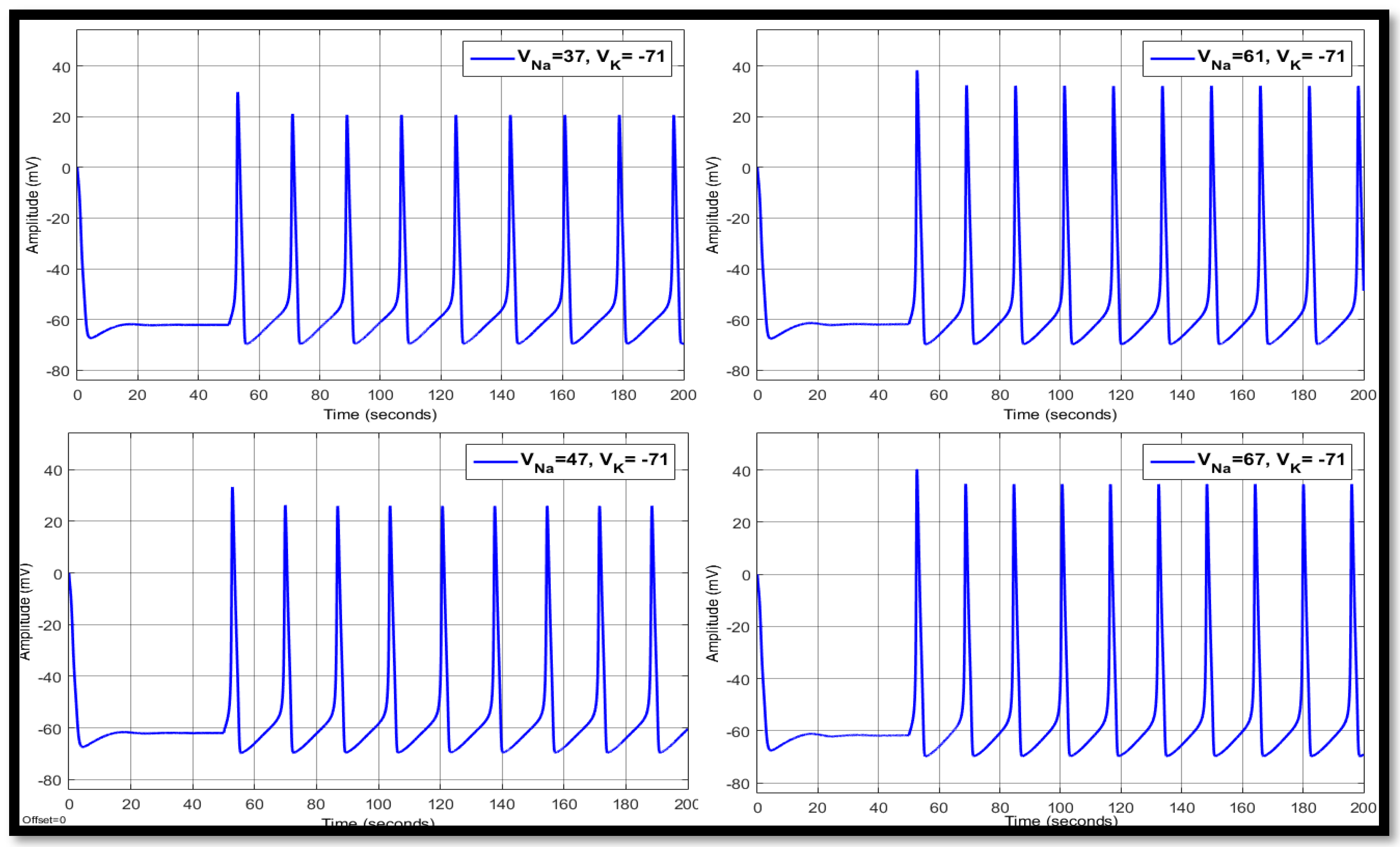
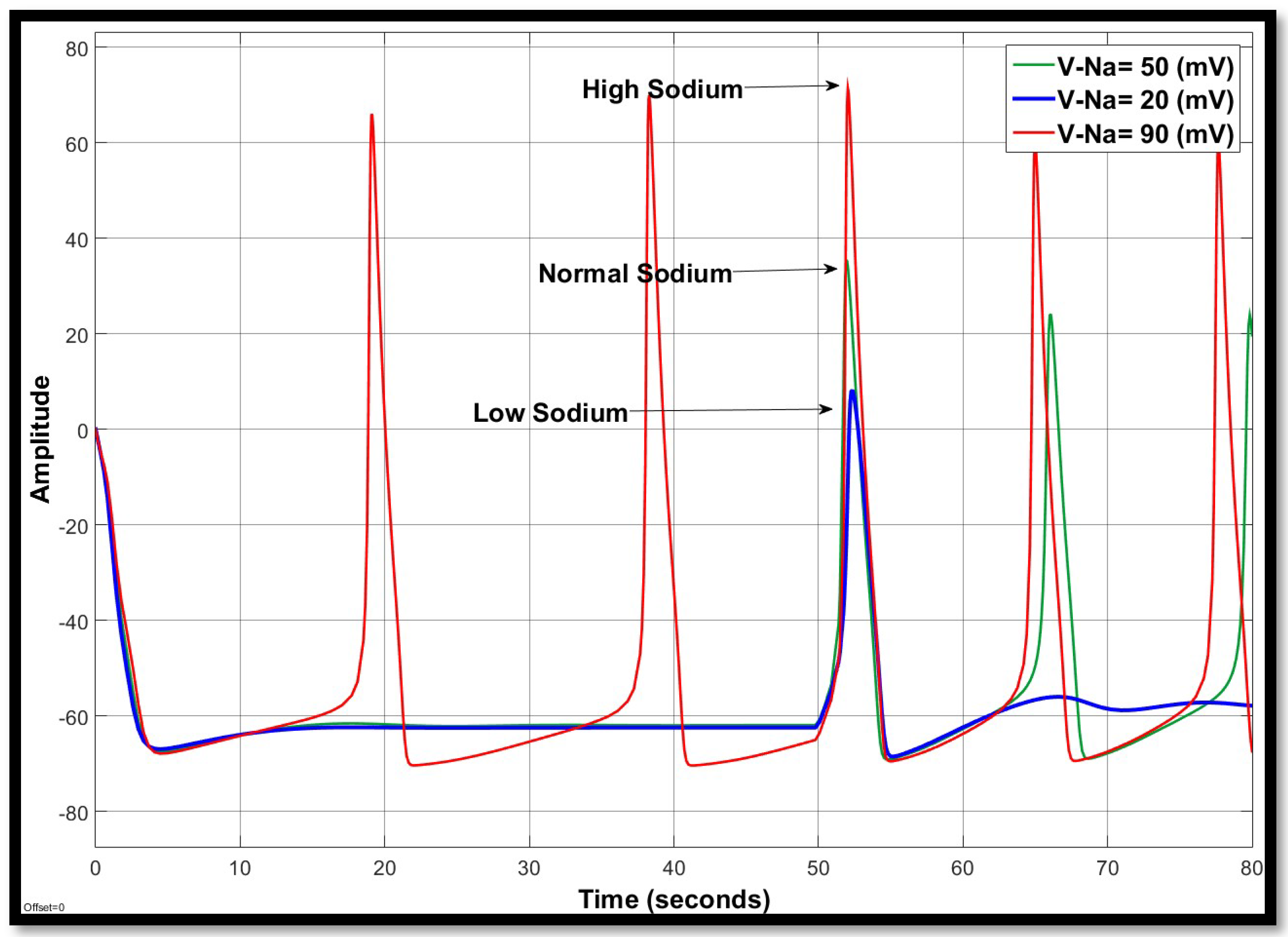
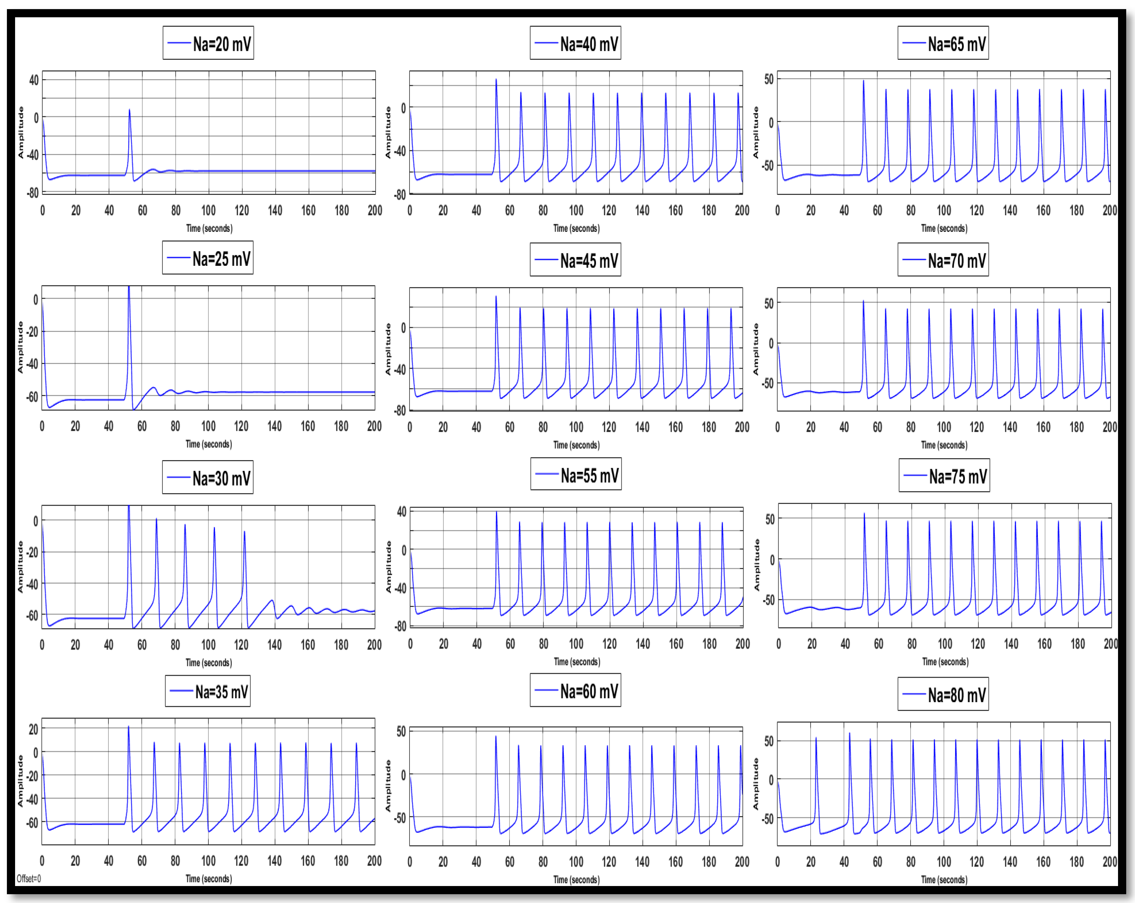
4.1.1. Sodium Ion Concentration Changes in a Single Neuron

The first set of results show the responses of the neuron to different levels of sodium ion concentrations in the neuron. The values were changed so that both hyper and hyponatremia were present. These are shown in Figure 7. The sodium potential was changed in stages from 20 mV to 80 mV. It can be seen that as the sodium ion concentration increased from its nominal value, the magnitudes of the spikes increased, while the inter-spike interval was reduced. In other words, the neurons responded with larger spikes at a more rapid rate. As the sodium concentration decreased, it can be seen that the magnitude of the spikes was suppressed to a point where there was no response from the neuron.

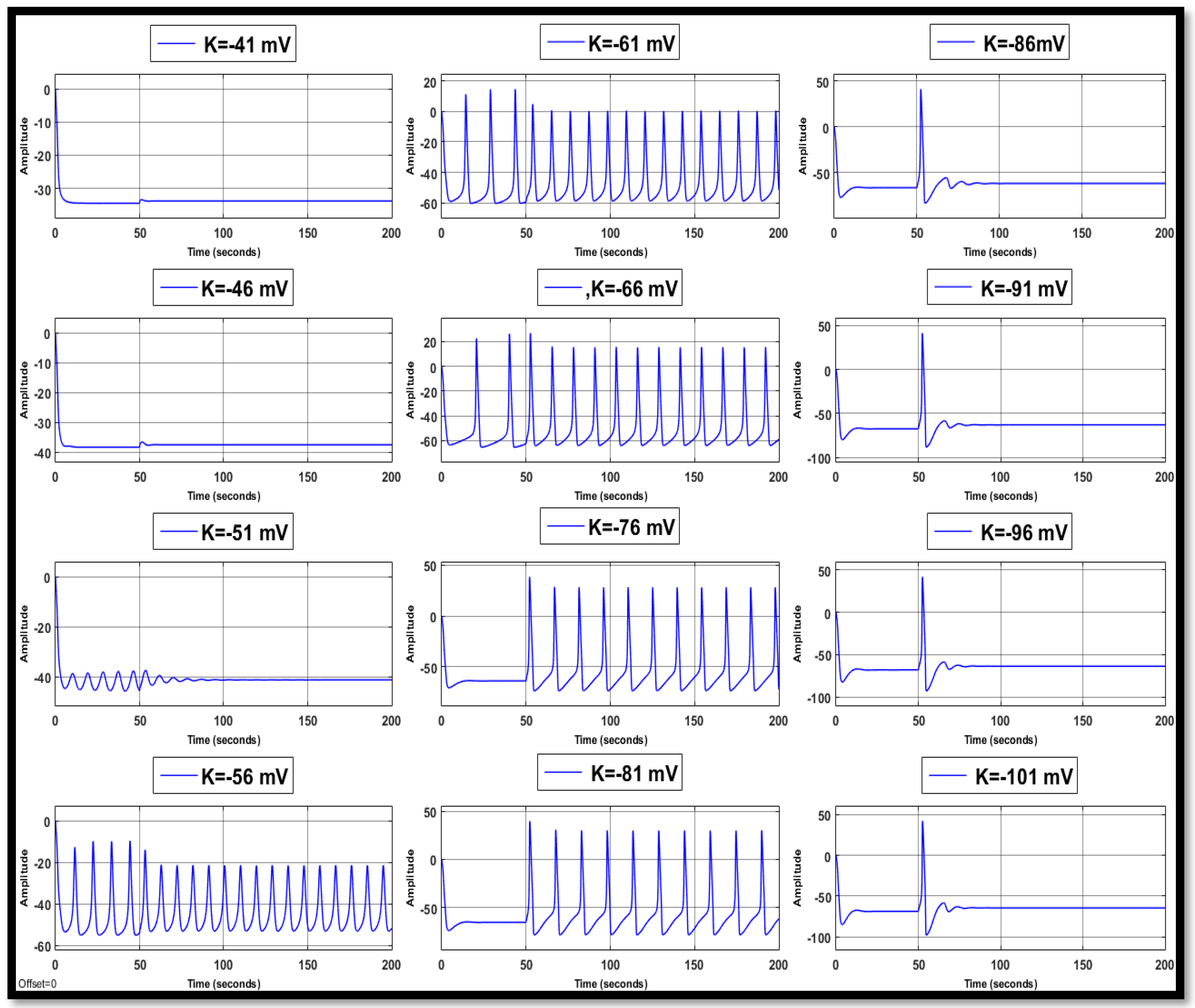
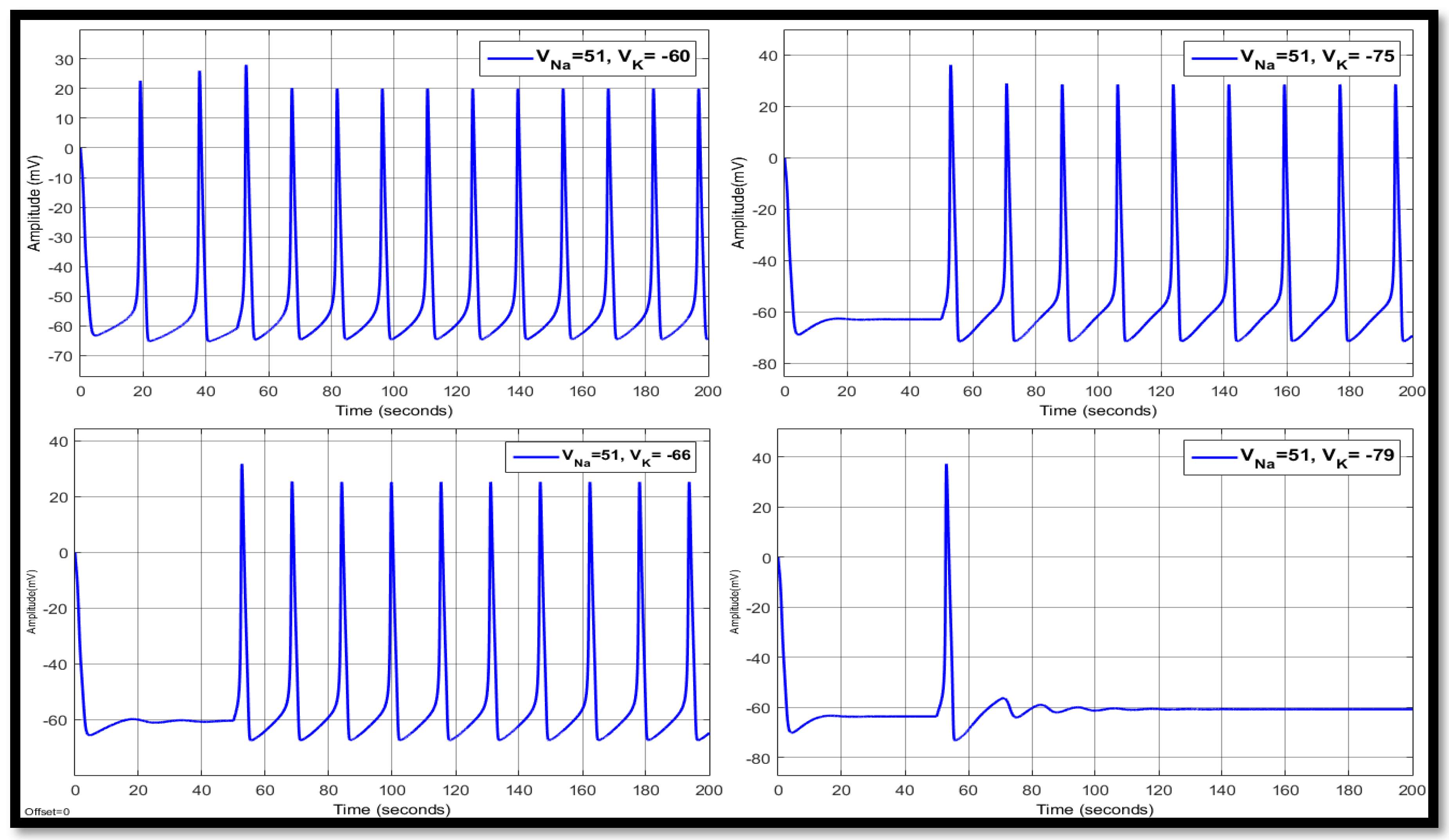
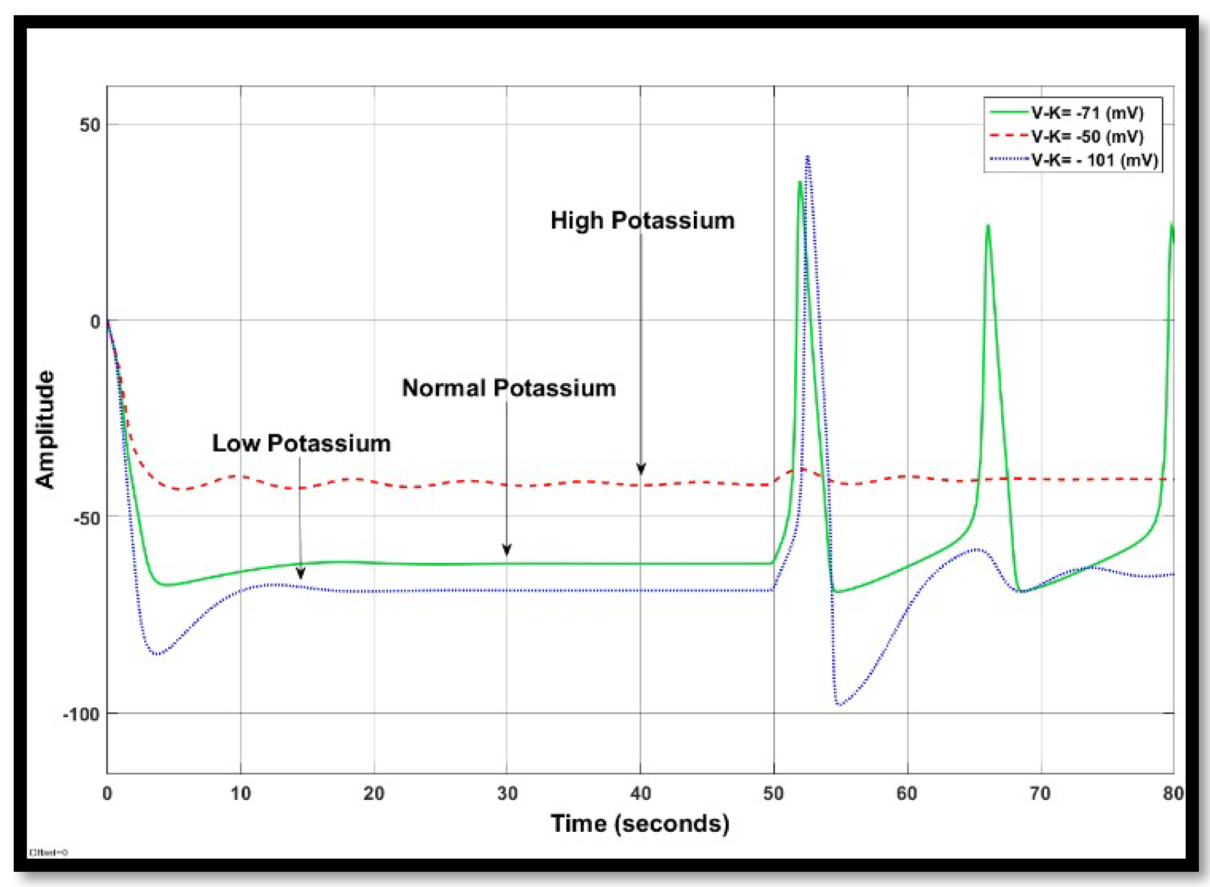
4.1.2. Changes in Potassium Concentration in a Single Neuron

We obtained results for the potassium ion concentration in the same way. These are shown in Figure 8. In the experiments, the effect of the changes in the potassium ion concentrations was more pronounced. Both an increase and decrease in potassium ion concentration lead to no response from the neuron. Thus, when V_K⁺ was −51 mV, the magnitude of the spikes was zero and there was no distinguishable inter-spike interval. A similar situation arose when V_K⁺ was below −76 mV. It should also be noted that these values are not that far from the nominal value of potassium which is −71 mV. This outcome indicates that the neuron is more sensitive to potassium ion changes than to sodium ion changes. The limits of these ranges can change if the parameters of the neuron are modified.

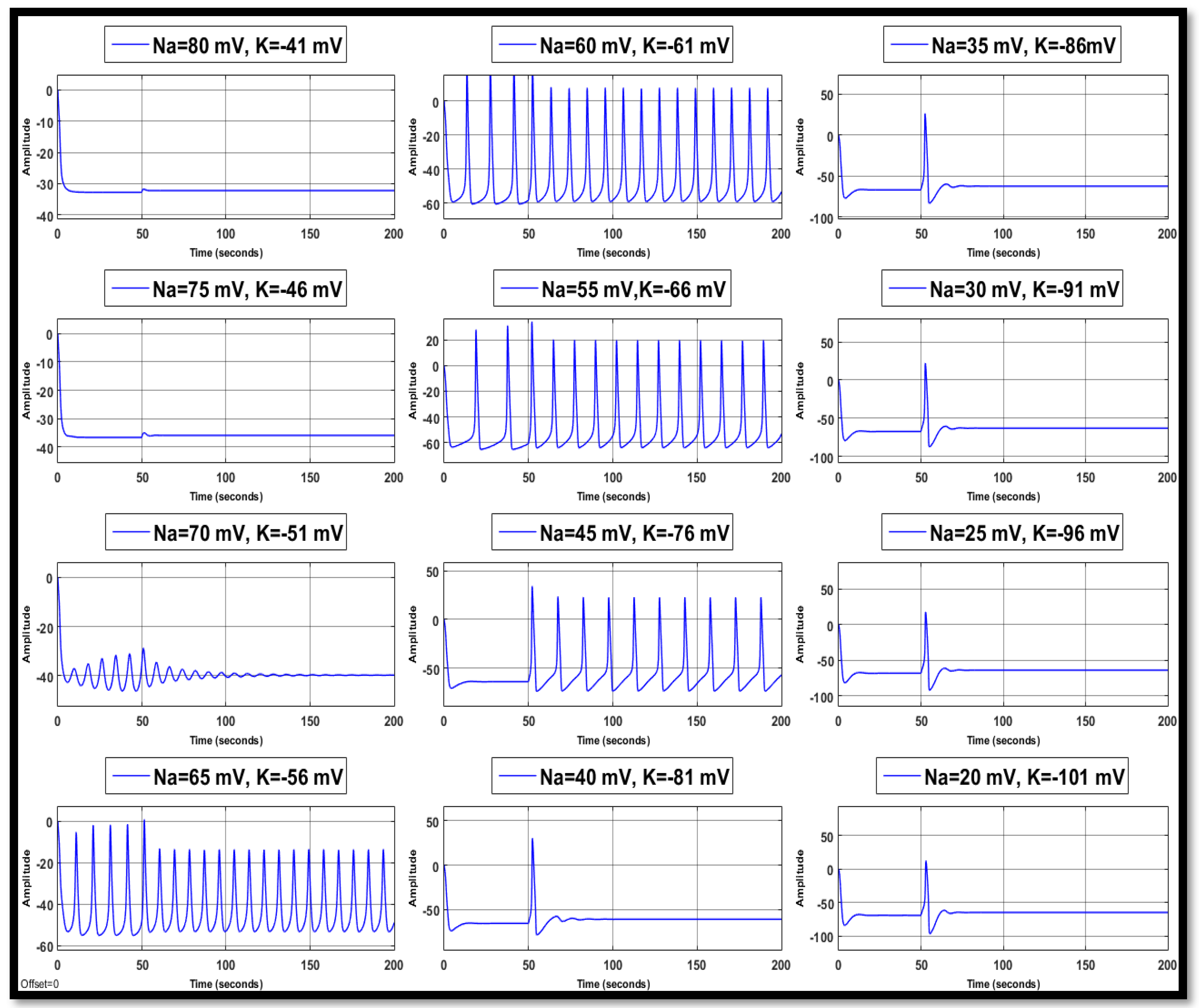
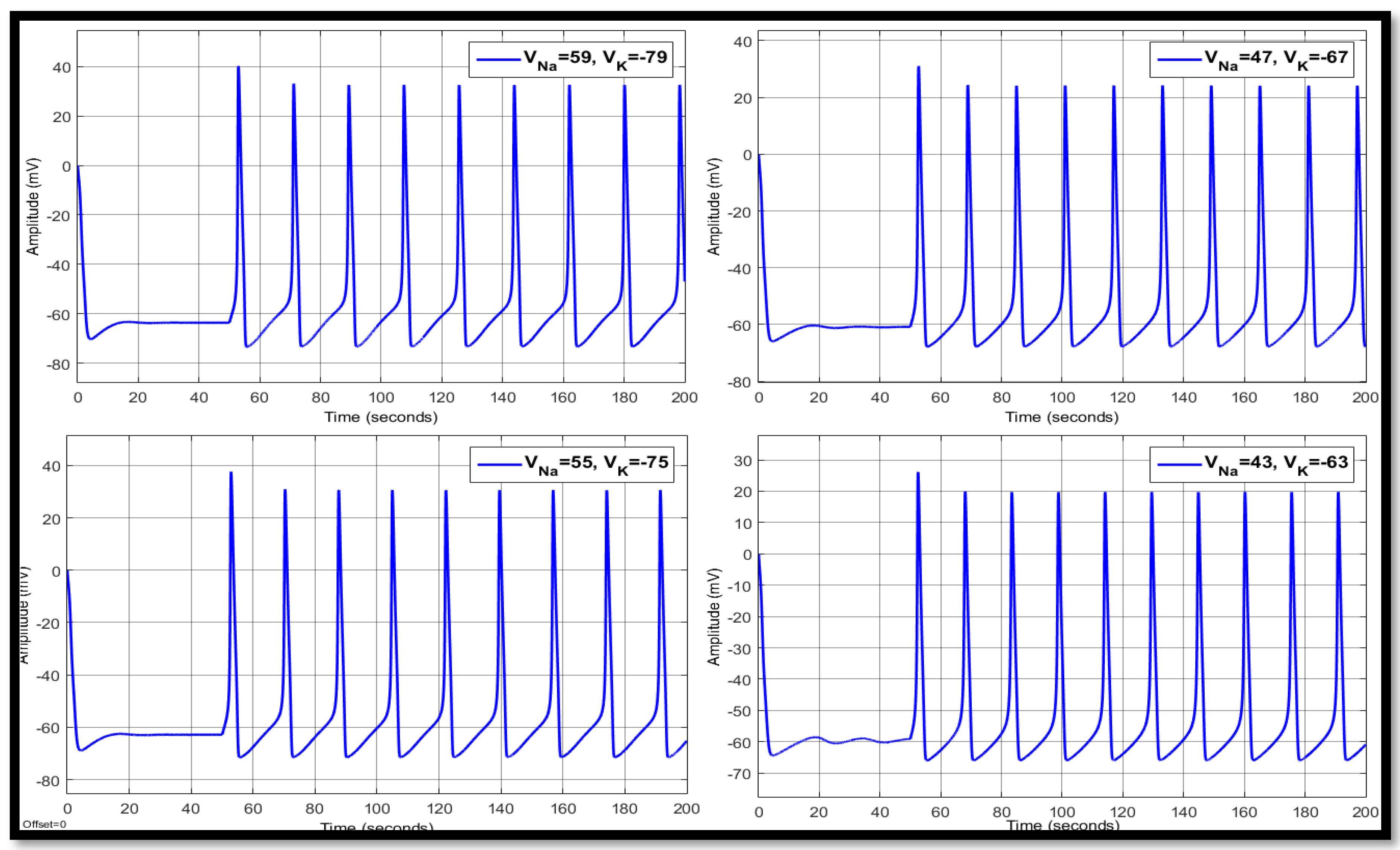
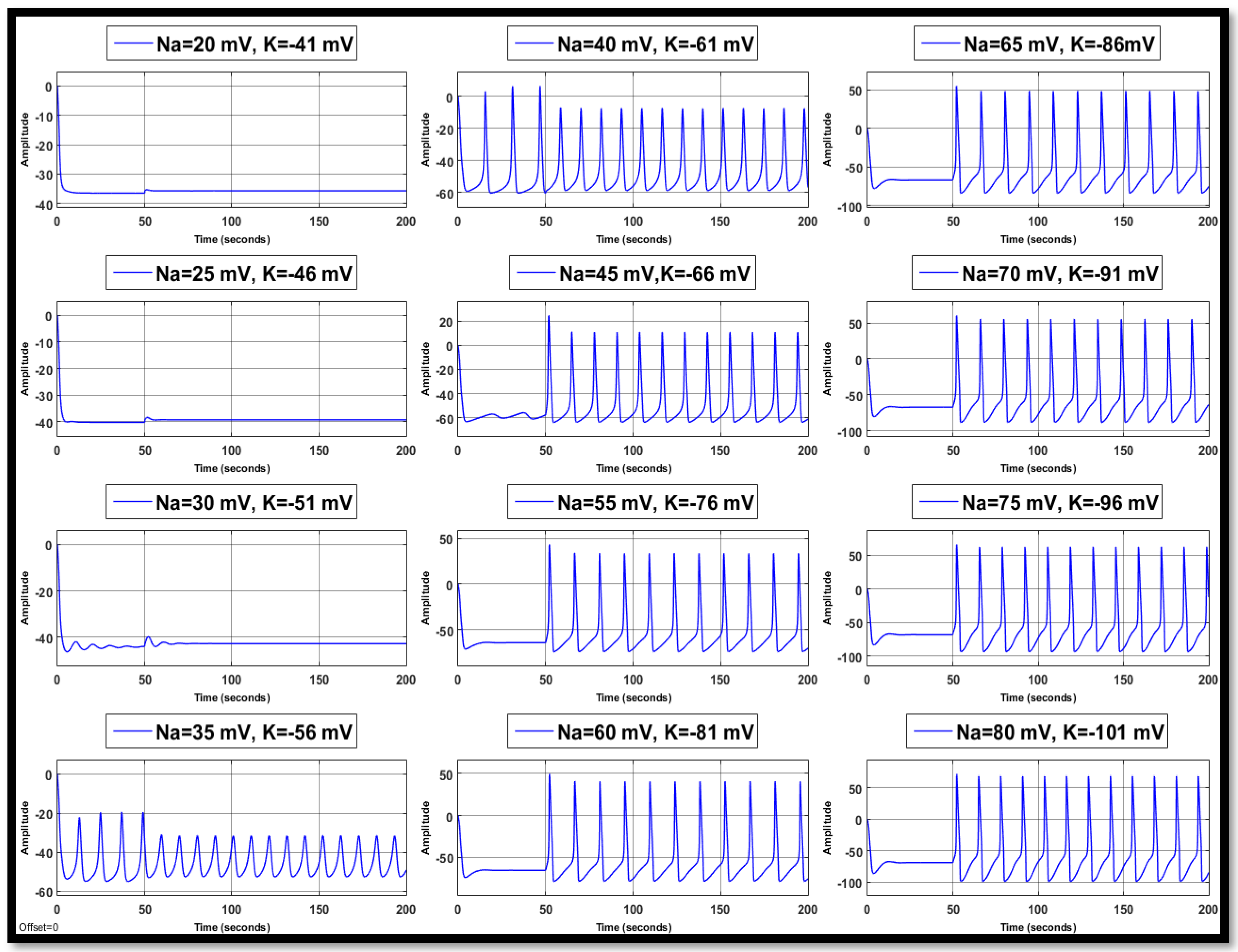
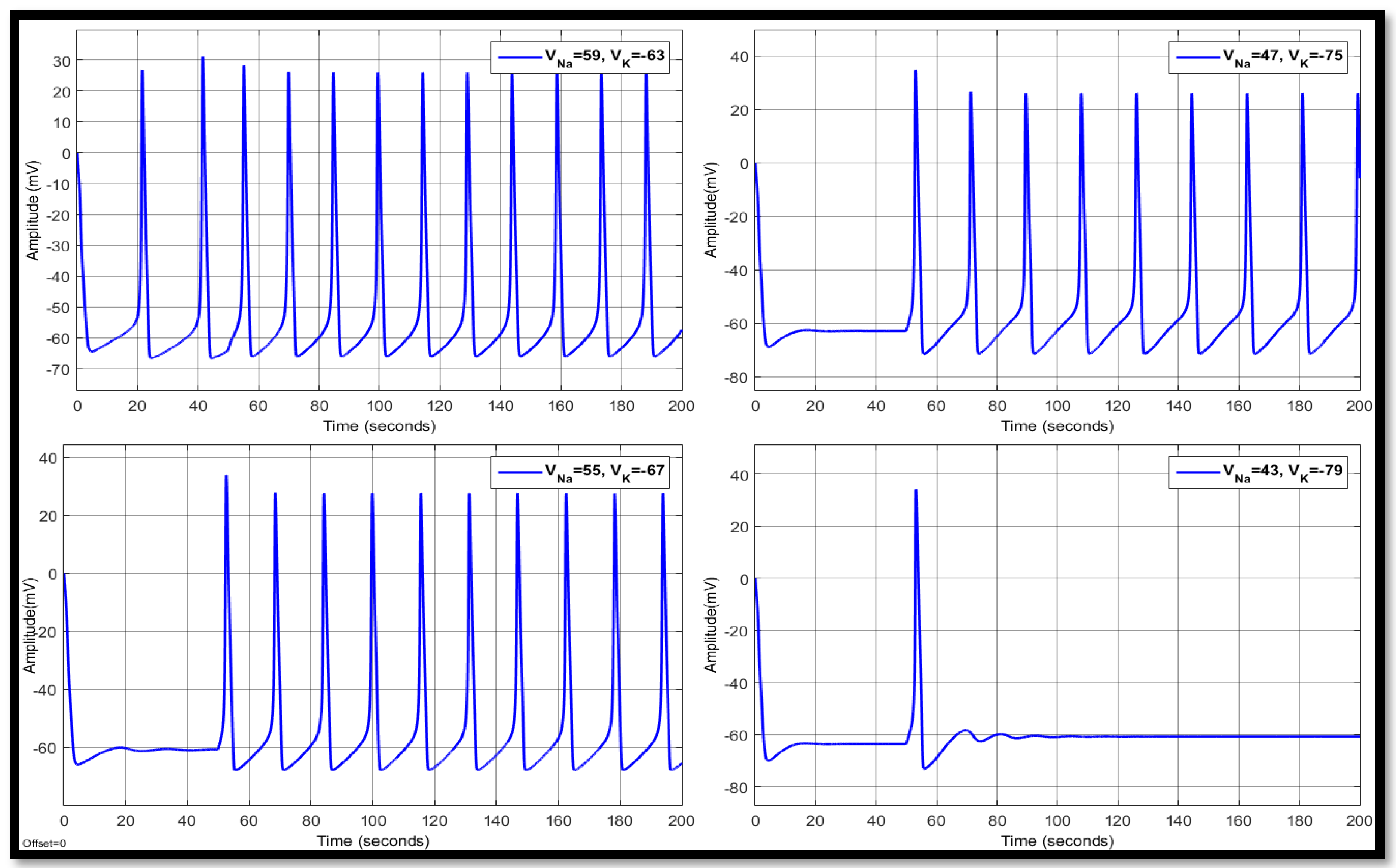
4.1.3. Combination of Changes in a Single Neuron

The next set of results relates to changes in the combination of sodium and potassium in a single neuron. Two different comparisons (a combination of both sodium and potassium changes) were carried out in order to investigate this particular situation. In the first part, the sodium potential was changed at various stages, from 61 mV to 41 mV, and the potassium potential was decreased from −61 mV to −81 mV, level by level. These results are shown in Figure 9 and Figure 10, below. From the results, it is clear that both sodium and potassium changes occurring at the same time affected almost every element of the action potentials, i.e., the inter-spike interval and the magnitude of the spikes. Results from these two figures can be compared with the results in Figure 8, which show that when combined ion changes occur in the neuron, the response is similar to the response when there is an imbalance in the potassium ion.

4.2. Ion Imbalances in Coupled Neurons

Neural populations in the nervous system consist of millions of individual neurons linked together through direct synaptic space. The action potential sent through the synaptic connections instructs the connected neurons to change their behavior, which effectively alters the phase of the connected neurons and brings them closer or further away from firing their signals [8]. It should be emphasized here that to simulate large-scale networks of spiking neurons the simple models are useful. Different level of ions and the structure of how neurons are connected in a network have a large impact on a multitude of synchronized behaviors. This set of experiments describes the nature of how ion imbalances affect the electrical dynamics of the connected neurons using the modelling of two conductance-based neurons. The two neurons had the same properties but the first neuron was suffering different kinds of electrolyte imbalance in each round of the experiment. The second neuron was in a healthy condition. From the experiments, it can be said that the timing between the firing of coupled neurons with a high value of coupling conductance is fixed, while this varies between uncoupled neurons and very weakly coupled neurons.

In the first experiment, the first neuron had sodium imbalances. In the second round, it had potassium imbalances. In the third round, it experienced both sodium and potassium imbalances, and, finally, the fourth round was the same as the third round but in reverse order for sodium and potassium imbalances (See Figure 11). Some of the critical characteristics of the action potential, like the average time intervals, the average peak intervals, and the average resting potential were investigated. For this reason, a train of action potentials for each round was run on the model in the 1000 s. The results for the various values of potassium and sodium and their combinations are shown in

Table 1. The average inter-spike intervals, spike amplitude and resting potential for sodium changes.

Ions		Single Faulty Neuron			Faulty Neuron in the Chain			Output of the Coupled Neuron
VNa	VK	Avg. Inter-Spike Intervals	Avg. Spike Amplitude	Avg. Resting Potential	Avg. Inter-Spike Intervals	Avg. Spike Amplitude	Avg. Resting Potential	Avg. Inter-Spike Intervals	Avg. Spike Amplitude	Avg. Resting Potential
37	−71	14.8758	10.5017	−63.147	17.9775	19.8064	−60.4662	17.9775	21.6552	−60.4557
47	−71	13.9576	21.0912	−62.7366	16.9507	26.3103	−59.9166	16.9468	26.7907	−59.9224
50	−71	13.7303	24.9737	−62.5314	16.7455	28.1351	−55.0608	16.7455	28.1554	−55.0897
61	−71	13.316	34.3568	−61.8532	16.1699	34.5527	−59.3163	16.1699	32.7097	−59.3666
67	−71	13.1332	39.8285	−61.3425	15.9336	38.0282	−59.0507	15.9336	35.1541	−59.1272

,

Table 2. The average inter-spike intervals, spike amplitude and resting potential for potassium changes.

Ions		Single Faulty Neuron			Faulty Neuron in the Chain			Output of the Coupled Neuron
VNa	VK	Avg. Inter-Spike Intervals	Avg. Spike Amplitude	Avg. Resting Potential	Avg. Inter-Spike Intervals	Avg. Spike Amplitude	Avg. Resting Potential	Avg. Inter-Spike Intervals	Avg. Spike Amplitude	Avg. Resting Potential
51	−60	10.7669	−2.0199	−50.6534	14.8411	21.2079	−52.9945	14.8411	20.8429	−53.3918
51	−66	12.7091	16.7945	−57.5069	15.7142	25.6603	−58.0945	15.7142	25.4610	−58.2092
50	−71	13.7303	24.9737	−62.5314	16.7455	28.1351	−55.0608	16.7455	28.1554	−55.0897
51	−75	14.3446	28.8061	−66.1146	17.8316	28.8506	−61.0727	17.8316	28.9676	−61.0148
51	−79	14.8463	31.0643	−69.3698	20.0183	31.2381	−61.9963	20.0183	31.4256	−61.9135

,

Table 3. The average inter-spike intervals, spike amplitude and resting potential for comparing hypernatremia with hyperkalemia and hyponatremia with hypokalemia.

Ions		Single Faulty Neuron			Faulty Neuron in the Chain			Output of the Coupled Neuron
VNa	VK	Avg. Inter-Spike Intervals	Avg. Spike Amplitude	Avg. Resting Potential	Avg. Inter-Spike Intervals	Avg. Spike Amplitude	Avg. Resting Potential	Avg. Inter-Spike Intervals	Avg. Spike Amplitude	Avg. Resting Potential
59	−63	11.5193	15.0944	−53.3364	15.1529	28.2043	−53.3745	15.1529	26.7059	−53.7817
55	−67	12.7956	22.3954	−58.2245	15.7045	29.0433	−58.2096	15.7045	29.0433	−58.2096
50	−71	13.7303	24.9737	−62.5314	16.7455	28.1351	−55.0608	16.7455	28.1554	−55.0897
47	−75	14.655	24.6221	−66.2517	18.2881	26.6333	−61.1840	18.2881	27.1293	−61.1367
43	−79	17.1933	22.2911	−69.5016	-	32.8146	−62.5148	-	34.3358	−62.4243

and

Table 4. The average inter-spike intervals, spike amplitude and resting potential for comparing hypernatremia with hypokalemia and hyponatremia with hyperkalemia.

Ions		Single Faulty Neuron			Faulty Neuron in the Chain			Output of the Coupled Neuron
VNa	VK	Avg. Inter-Spike Intervals	Avg. Spike Amplitude	Avg. Resting Potential	Avg. Inter-Spike Intervals	Avg. Spike Amplitude	Avg. Resting Potential	Avg. Inter-Spike Intervals	Avg. Spike Amplitude	Avg. Resting Potential
59	−79	14.2584	39.5384	−69.0874	18.1669	34.9578	−61.8693	18.1669	33.5213	−61.8110
55	−75	14.109	32.8513	−65.9258	17.3166	32.2044	−60.6708	17.3166	31.4881	−60.6250
50	−71	13.7303	24.9737	−62.5314	16.7455	28.1351	−55.0608	16.7455	28.1554	−55.0897
47	−67	13.0706	15.0905	−58.852	16.0560	24.5569	−58.7456	16.0560	24.8891	−58.8273
43	−63	12.2359	2.2251	−54.8835	15.3754	19.6940	−57.1269	15.3791	20.3892	−57.2454

and Figure 12, Figure 13, Figure 14 and Figure 15. The tables consist of three sections. The first part represents the results for changes in the single neuron. The second section lists the results of the first neuron in the coupling condition. Finally, the third part of the table reveals the functions of the second neuron and the outputs of the system in the coupling state.

The results for the coupled model for both hyper and hyponatremia are presented in Table 1 and Figure 12, below.

The results for both hyper and hypokalemia are presented in Table 2 and Figure 13, below.

Finally, the results for hyper and hyponatremia plus hyper and hypokalemia at the same time are represented in Table 3 and Table 4.

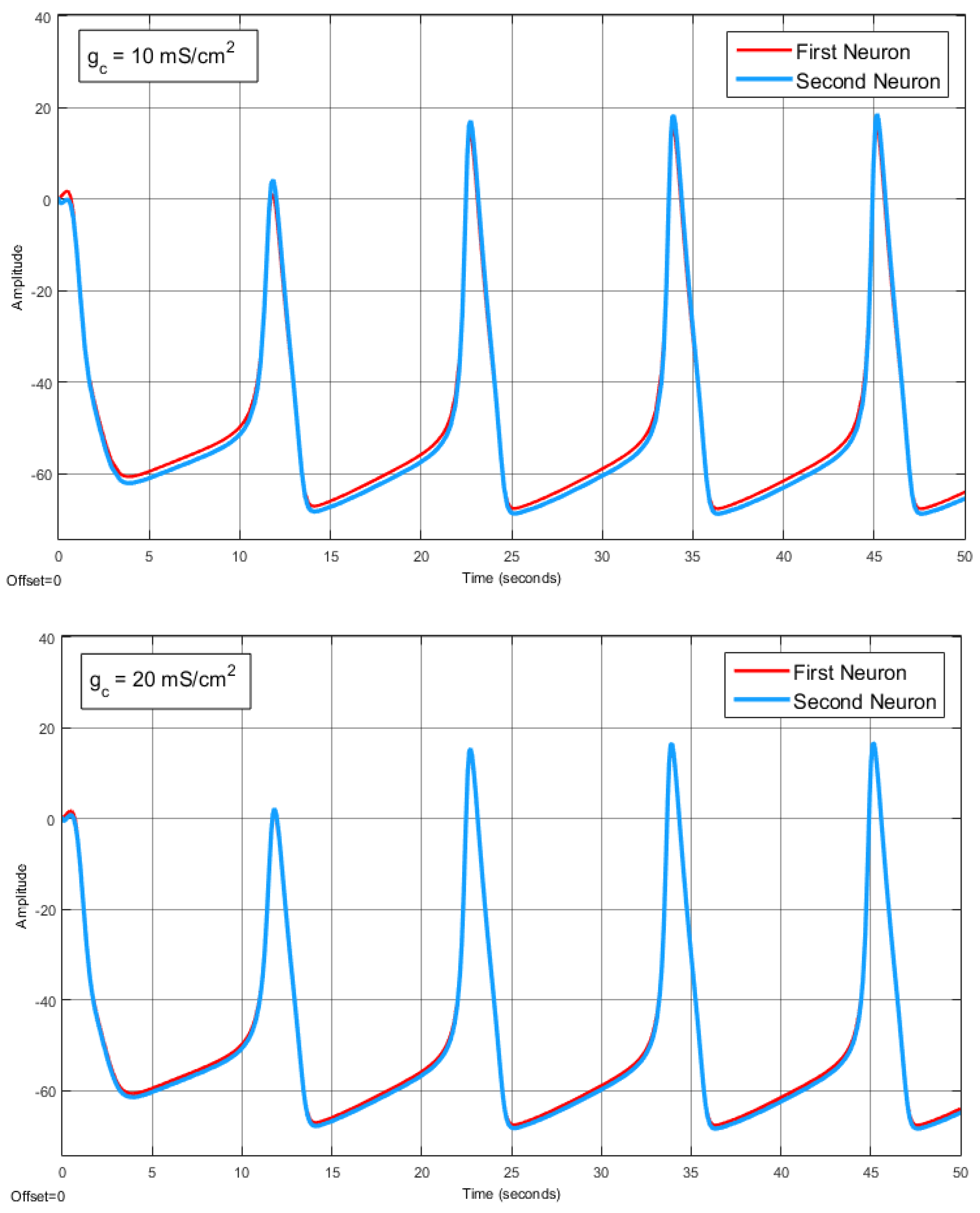
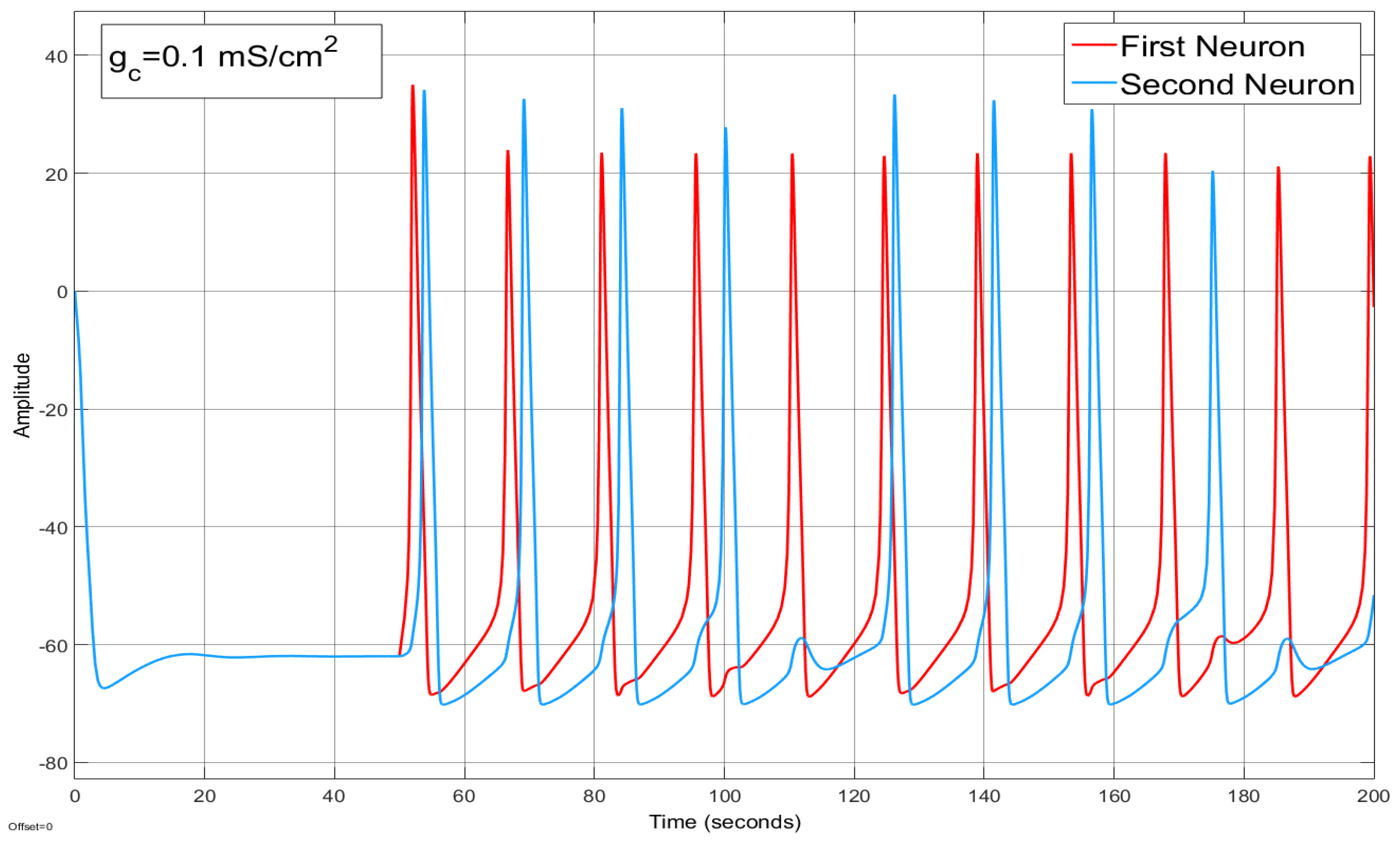
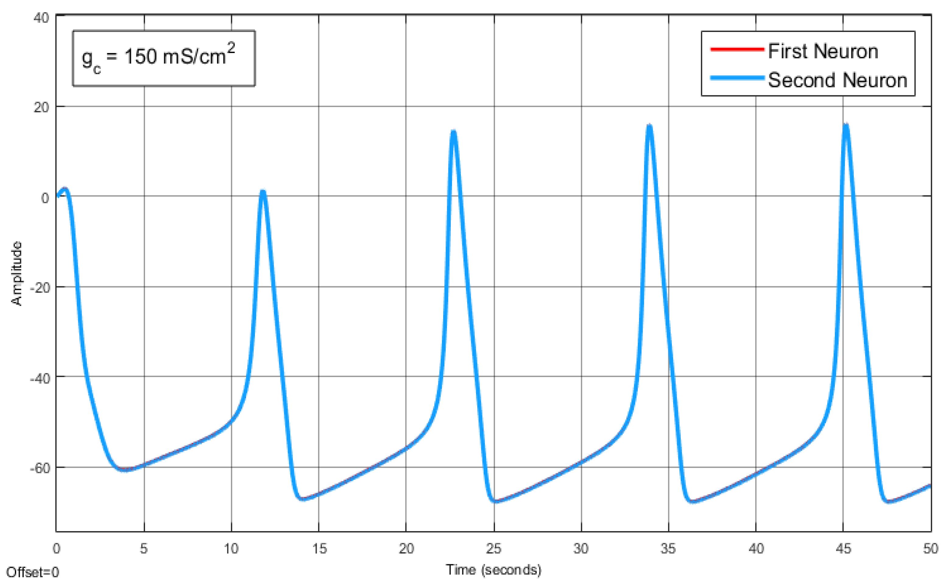
The Effect of Coupling Conductance on Synchronization

How big should coupling conductance be? Previously, in Section 3.4, the minimum current for synchronization was suggested. As is shown in Equation (30), the minimum current $I_c$ for the second neuron has to be at least $\frac{I_{inj1}}{2}$. As $I_c=\Delta V·g_c$, the value f $g_c$ is crucial for synchronization. The experiments showed that, by increasing $g_c$, the synchronicity in coupling became stronger. Figure 16 shows the results. As the results show, increasing the coupling parameters or coupling conductance further leads to a globally synchronous regime.

As coupling conductance increased, synchronization was triggered. After further coupling, conductance, increasing both action potentials, coincided, with some slight defects. As the results show, by picking sufficiently large coupling conductance, cell synchronization occurred. The reason behind increasing the synchronicity of coupled neurons was to increase the coupling conductance of $g_c$ and relate it to the nature of $g_c$. By considering the relation of $g_c$ with its resistance, which is $g_c=\frac{1}{R}$, we concluded that increasing the coupling conductance causes a decrease in the resistance between two neurons; and that by decreasing the resistance between two neurons, the neurons become more synchronized.

5. Discussion

The computational models applied in this paper are simple circuits which integrate differential equations representing abnormalities in the different levels of electrolyte potential for single and coupled neurons. The model easily sits in a regime that reproduces the same action potential as the firing patterns observed in biological neurons. The preliminary results showed that the fast and slow action potentials were related to the properties of internal settings of the neuron. The range of observations summarized in Figure 6, Figure 7, Figure 8, Figure 9 and Figure 10 show the response and complexity of configurations for a single neuron. However, coupled neurons show more complex behaviors (See Figure 12, Figure 13, Figure 14, Figure 15 and Figure 16).

Responses to the combined effect of the concentrations of the sodium and potassium ions in the neuron for single or coupled neurons are presented in Figure 9, Figure 10, Figure 14, and Figure 15. This understanding can help, in the understanding of neurodegenerative diseases, e.g., tremors, motor neuron diseases, Parkinson’s, and Alzheimer’s disease. The reason for this is that intracellular and extracellular potassium and sodium concentrations play a vital role in the electrophysiological function of the body and the neurons that control it. These two ions are essential in maintaining cellular homeostasis and most metabolic processes are dependent on or affected by these electrolytes. There is a significant relationship between sodium and potassium changes and the level of the action potential and resting potential. As in the results of earlier experiments carried out on the model, it could be seen that increasing the concentration of potassium raises resting potential toward threshold and, in contrast, decreasing the concentration of potassium lowers resting potential away from threshold. In the same way, increasing the concentration of sodium raises the level of action potential more positive. Inversely, decreasing the concentration of sodium reduces the level of action potential more negative. Figure 17 and Figure 18 summarize the behavior of neurons in the course of sodium and potassium changes in the experiments.

During the combination of sodium and potassium imbalances, the conditions led to the properties of potassium concentration (see Figure 7 and Figure 8 and Table 3 and Table 4). This means that the important features of an action potential, like the rate of rising of the action potential, its peak amplitude, and its duration, are more dependent on the properties of potassium. By pointing out this biological fact, a possible explanation for these observations could be related to the concentrations of sodium and potassium. The normal concentration of sodium in the blood serum is 136–146 mMol/L and the normal potassium level is 3.5–5 mMol/L [31]. Therefore, it can be interpreted that, as the amount of sodium is much more than the amount of potassium (around 39 times), changing only a small amount of potassium can have a significant impact on the volume of its total amount, while the reduction of small volumes of sodium does not have a large impact on the total volume [32]. For this reason, it can be seen that during the combination of sodium and potassium imbalances the impact of potassium on neuronal functions was much stronger than sodium.

Another interesting characteristic was the impact of coupling conductance on the synchronicity of coupled neurons. The results indicate that any changes in the coupling conductance can drive the neurons to different degrees of synchronization. These results are displayed in Figure 16. In general, the experiments with the coupling conductance contribute directly to our understanding of the origin of synchronization in a network of neurons through regularization of the conductance.

Some characteristics of action potentials displayed considerable changes during the experiments for coupled neurons in comparison to firing the single neuron. This model study has shown that electrical coupling can either increase or decrease the frequency of action potentials. The results in Figure 16 demonstrate that coupling conductance, g_c, and properties of the postsynaptic signal of membranes can greatly influence the frequency changes in the coupled neurons. The coupling between two neurons is variable; it increases any time the two neurons are simultaneously active. From a computational point of view, this can be interpreted through Equation (25), where two neurons are simultaneously active, p₁ = p₂. The results demonstrated that coupling effected the average spike amplitudes and the average resting potentials as well. Table 1, Table 2, Table 3 and Table 4 show that, after applying coupling parameters on the model, the average spike amplitudes and the average resting potential became greater than the same condition in the single neuron. On the other hand, comparing the experiments of the single neuron, presented in Figure 6, Figure 7, Figure 8, Figure 9 and Figure 10, with coupled neurons, Table 1, Table 2, Table 3 and Table 4, revealed that coupled neurons could shape the frequency and waveform of the action potential. The experiments also revealed coupling maxima between neurons when both neurons had the same settings (i.e., the same level of sodium and potassium ions).

References

1. Sadegh Zadeh, S.-A.; Kambhampati, C. A Computational Investigation of the Role of Ion Gradients in Signal Generation in Neurons. In Proceedings of the Computing Conference, London, UK, 10–12 July 2018. [Google Scholar]
2. Amthor, F.; Oyster, C.; Takahashi, E. Morphology of on-off direction-selective ganglion cells in the rabbit retina. Brain Res. 1984, 298, 187–190. [Google Scholar] [CrossRef]
3. Ahmed, B.; Allison, J.D.; Douglas, R.J.; Martin, K. An intracellular study of the contrast-dependence of neuronal activity in cat visual cortex. Cereb. Cortex 1997, 7, 559–570. [Google Scholar] [CrossRef] [PubMed] [Green Version]
4. Dodge, J. A Study of Ionic Permeability Changes Underlying Excitation in Myelinated Nerve Fibers of the Frog. Ph.D. Thesis, Rockefeller Institute, New York, NY, USA, 1967. [Google Scholar]
5. Hodgkin, A.; Huxley, A. A quantitative description of membrane current and its application toconduction and excitation in nerve. J. Physiol. 1952, 117, 500–544. [Google Scholar] [CrossRef]
6. Matsuda, K.; Hoshi, T.; Kameyama, S. Electrophysiology of the heart. J. Exp. Med. 1958, 66. [Google Scholar]
7. Raman, I.; Bean, B. Ionic Currents Underlying Spontaneous Action Potentials in Isolated Cerebellar Purkinje Neurons. J. Neurosci. 1999, 19, 1663–1674. [Google Scholar] [CrossRef] [Green Version]
8. Sadegh Zadeh, S.-A.; Kambhampati, C. All-or-None Principle and Weakness of Hodgkin-Huxley Mathematical Model. In Proceedings of the 19th International Conference on Systems Biology and Bioengineering, Chicago, IL, USA, 26–27 October 2017. [Google Scholar]
9. Cleeremans, A. Connecting Conscious and Unconscious Processing. Cogn. Sci. 2014, 38, 1286–1315. [Google Scholar] [CrossRef] [PubMed]
10. Trenor, B.; Cardona, K.; Saiz, J.; Noble, D.; Giles, W. Cardiac action potential repolarization re-visited: Early repolarization shows all-or-none behaviour. J. Physiol. 2017, 595, 6599–6612. [Google Scholar] [CrossRef] [PubMed]
11. Engel, J.; Pedley, T.; Aicardi, J. Epilepsy: A Comprehensive Textbook; Lippincott-Raven: Philadelphia, PA, USA, 2008. [Google Scholar]
12. Singer, W. Neurobiology: Striving for coherence. Nature 1999, 397, 391–393. [Google Scholar] [CrossRef]
13. Borgesa, R.; Borges, F.S.; Lameu, E.L.; Batista, A.M.; Iarosz, K.C.; Caldas, I.L.; Viana, R.L.; Sanjuán, M.A.F. Effects of the spike timing-dependent plasticity on the synchronisation in a random Hodgkin–Huxley neuronal network. Commun. Nonlinear Sci. Numer. Simul. 2016, 34, 12–22. [Google Scholar] [CrossRef] [Green Version]
14. Prado Tde, L.; Lopes, S.R.; Batista, C.A.; Kurths, J.; Viana, R.L. Synchronization of bursting Hodgkin-Huxley-type neurons in clustered networks. Phys. Rev. E 2014, 90, 032818. [Google Scholar] [CrossRef] [PubMed]
15. Hansel, D.; Mato, G.; Meunier, C. Synchrony in Excitatory Neural Networks. Neural Comput. 1995, 7, 307–337. [Google Scholar] [CrossRef]
16. Belykh, V.N.; Osipov, G.V.; Petrov, V.S.; Suykens, J.A.K.; Vandewalle, J. Cluster synchronization in oscillatory networks. Chaos 2008, 18, 037106-1–037106-6. [Google Scholar] [CrossRef] [PubMed]
17. Batistaa, C.; Lopesa, S.; Vianaa, R.; Batistab, A. Delayed feedback control of bursting synchronization in a scale-free neuronal network. Neural Netw. 2010, 23, 114–124. [Google Scholar] [CrossRef]
18. Han, F.; Wiercigroch, M.; Fang, J.-A.; Wang, Z. Excitement and synchronization of small-world neuronal networks with short-term synaptic plasticity. Int. J. Neural Syst. 2011, 21, 415–425. [Google Scholar] [CrossRef] [PubMed]
19. Gray, C.M.; Konig, P.; Engel, A.K.; Singer, W. Oscillatory responses in cat visual cortex exhibit inter-columnar synchronization which reflects global stimulus properties. Nature 1989, 338, 334–337. [Google Scholar] [CrossRef] [PubMed]
20. Stopfe, M.; Bhagavan, S.; Smith, B.; Laurent, G. Impaired odour descrimination on desynchronization of odour-encoding neural assemblies. Nature 1997, 390, 70–74. [Google Scholar] [CrossRef] [PubMed]
21. Steinmetz, P.; Roy, A.; Fitzgerald, P.J.; Hsiao, S.S.; Johnson, K.O.; Niebur, E. Attention modulates synchronized neuronal firing in primate somatosensory cortex. Nature 2000, 404, 187–190. [Google Scholar] [CrossRef]
22. Stern, E.; Jaeger, D.; Wilson, C.J. Membrane potential synchrony of simultaneously recorded striatal spiny neurons in vivo. Nature 1998, 394, 475–478. [Google Scholar] [CrossRef] [PubMed] [Green Version]
23. Hodgkin, A.; Huxley, A. Currents carried by sodium and potassium ions through the membrane of the giant axon of Loligo. J. Physiol. 1952, 116, 49–472. [Google Scholar] [CrossRef]
24. Whelton, P. Hyponatremia in the general population. What does it mean? PubMed 2016, 26, 9–12. [Google Scholar] [CrossRef]
25. Silva, A.; Belli, A.; Smith, M. Electrolyte and endocrine disturbances. In Oxford Textbook of Neurocritical Care; Kofke, A., Ed.; Oxford Medicine Online: Oxford, UK, 2016; pp. 375–386. [Google Scholar]
26. Perez, C.; Ziburkus, J.; Ullah, G. Analyzing and Modeling the Dysfunction of Inhibitory Neurons in Alzheimer’s Disease. PLoS ONE 2016, 11, 1–24. [Google Scholar] [CrossRef] [PubMed]
27. Labouriau, I.S.; Ruas, M.A.S. Singularities of equations of Hodgkin–Huxley type. Dyn. Stabil. Syst. 1996, 11, 91–108. [Google Scholar] [CrossRef]
28. Labouriau, I.; Rodrigues, H.M. Synchronization of Coupled Equations of Hodgkin-Huxley Type. Dyn. Contin. Discret. Impuls. Syst. Ser. A 2003, 10, 463–476. [Google Scholar]
29. Pikovsky, A.; Rosenblum, M.; Kurths, J. Synchronization: A Universal Concept in Nonlinear, 1st ed.; Cambridge University: Cambridge, UK, 2003. [Google Scholar]
30. Rossetto, M. A note on the falsification of the ionic theory of hair cell transduction. Commun. Integrat. Biol. 2016, 9, e1122144. [Google Scholar] [CrossRef]
31. Kashyap, C.; Borkotoki, S.; Dutta, R.K. Study of Serum Sodium and Potassium Level in Patients with Alcoholic Liver Disease Attending Jorhat Medical College Hospital—A Hospital Based Study. Int. J. Health Sci. Res. 2016, 6, 113–116. [Google Scholar]
32. Sadegh-Zadeh, S.-A.; Kambhampati, C. Computational Investigation of Amyloid Peptide Channels in Alzheimer’s Disease. J 2019, 2, 1–14. [Google Scholar] [CrossRef]
Figure 1. The structure of a neuron. Most neurons in the vertebrate nervous system have the same structure.
J 02 00003 g001
Figure 2. Recording a transmembrane potential during depolarization and repolarization of a nerve fiber. The different phases of the action potential are presented as follows: Vm is transmembrane voltage, PNa is membrane permeability to sodium, and PK is membrane permeability to potassium. The relative membrane permeability relationships between potassium and sodium ions associated with each of the phases are shown. For instance, PNa >> PK means that permeability for Na is greater than permeability for K, where > means greater and >> means much greater.
J 02 00003 g002
Figure 3. The schemes of coupling in neural networks. (a) Full connectivity: a network of nine neurons with all-to-all coupling. The input links are shown for two representative neurons. Self-couplings are not indicated. (b) Random coupling with fixed connection probability. The input links are larger than in a network with the population of nine. (c) Random coupling with a fixed number of inputs. The number of connections from input links to two representative neurons does not change when the size of the network is increased.
J 02 00003 g003
Figure 4. Neuronal circuitry with electrical and chemical synapses. (a) A model of electrically coupled neurons and (b) a model of chemically connected neurons.
J 02 00003 g004
Figure 5. Couplings between neurons. Schematic representation of the signaling of electrical coupling in neurons.
J 02 00003 g005
Figure 6. The running of experiments for three single neurons without any changes. All three graphs have been overlapped. VNa+ = 50 mV, VK+ = −71 mV.
J 02 00003 g006
Figure 7. Sodium changes and the responses of a neuron in the course of hypernatremia and hyponatremia. The potassium value for all of these experiments remained normal, VK+ = −71.
J 02 00003 g007
Figure 8. Potassium changes and the responses of neurons in the course of hyperkalemia and hypokalemia. The sodium value for all of these experiments remained normal, VNa+ = 50.
J 02 00003 g008
Figure 9. Sodium and potassium changes and the responses of neurons in the course of hypernatremia-hyperkalemia and hyponatremia-hypokalemia.
J 02 00003 g009
Figure 10. Sodium and potassium changes and the responses of neurons in the course of hyponatremia-hyperkalemia hypernatremia-hypokalemia.
J 02 00003 g010
Figure 11. In some neurological diseases, the neuron’s entire neural network in the nervous system does not work properly. The affected nerve cells have a problem transmitting signals from one area of the brain to another or, even, can no longer do it. Here, this problem here is simulated on a very small scale. The first neuron works as a faulty neuron and the second one works as a healthy neuron’s entire neural network.
J 02 00003 g011
Figure 12. Sodium changes and the responses of coupled neurons in the course of hypernatremia and hyponatremia. The potassium value for all of these experiments remained normal, VK+ = −71.
J 02 00003 g012
Figure 13. Potassium changes and the responses of coupled neurons in the course of hyperkalemia and hypokalemia. The sodium value for all of these experiments remained normal, VNa+ = 50.
J 02 00003 g013
Figure 14. Sodium and potassium changes and the responses of coupled neurons in the course of hypernatremia-hyperkalemia and hyponatremia- hypokalemia.
J 02 00003 g014
Figure 15. Sodium and potassium changes and the responses of coupled neurons in the course of hyponatremia-hyperkalemia and hypernatremia-hypokalemia.
J 02 00003 g015
Figure 16. Increasing the coupling conductance. The results were obtained from a coupled Hodgkin–Huxley neural model in which the coupling conductance was progressively increased in the steps. The current injection for this experiment was 20 mA.
J 02 00003 g016aJ 02 00003 g016bJ 02 00003 g016c
Figure 17. Increasing extracellular levels of potassium means more K+ enters the cell and the resting potential goes up. In comparison, decreasing the extracellular level of potassium means more net K+ leaves the cell and the resting potential goes down.
J 02 00003 g017
Figure 18. The effects of changes in the plasma Na+ concentration on the action potential. Increasing the extracellular level of sodium causes the nerve action potential to have a higher peak and to occur faster. Conversely, decreasing the extracellular concentration of Na+ will have the inverse effect.
J 02 00003 g018