Revisiting the Relationship between Financial Wealth, Housing Wealth, and Consumption: A Panel Analysis for the U.S.

Abstract

Based on the seminal paper of Case, Quigley, and Shiller (2013), we investigated the effects of financial and housing wealth on consumption. Using quarterly data from 1975 to 2016 for all states of the U.S. economy, and a different methodology in measuring wealth, we report relatively greater financial effects than housing effects on consumption. Specifically, in our basic utilized model, the calculated elasticity for financial wealth was 0.060, while for housing it was 0.045. The results were not in agreement with the ones obtained by Case, Quigley, and Shiller. In an attempt to investigate this disparity, we proceeded by incorporating the introduction of the Tax Reform Act in 1986, which increased incentives for owner-occupied housing investments. Finally, due to distributional factors at work, and taking into account the pronounced uneven distribution of wealth, we investigated the effects of wealth for eight states that included the metropolitan areas comprising the well-known Case–Shiller 10 City Composite Index. Now the housing effect on consumption was much stronger and larger than the financial effect. Additionally, we forecasted the consumption changes at the time of high rise and large drops in house prices for these states. Forecasts showed a recession from the fall of Lehman Brothers until the fourth quarter of 2011. These forecasts were not verified. Probably, the new techniques used by policies played an important role. We also found that extreme behaviors cannot be predicted.

1. Introduction

The pronounced volatility in the prices of financial assets and in housing prices during the period from 2002 to 2009, and consequently the effects of the Great Recession on the economy has led to renewed political and scientific interest in the effect of wealth on aggregate consumption. The enormous swings in wealth, either from financial wealth or property wealth have grown in importance and raised a number of questions about the macroeconomic implications on consumer spending, aggregate demand, and consequently on economic activity. Declines in stock prices accelerate the slowdown of household consumption, and thus, of economic activity, a process which eventually could lead to a recession. The same importance yields changes in housing wealth upon household behavior, since recent developments in the housing markets give the opportunity to the homeowner to extract cash from housing and use it for consumption.

Against this backdrop, it is not surprisingly that some researchers state that housing equity is essentially similar to the act of selling shares. But in contrast to that, other researchers point out that the impact of stock market wealth accumulation may be quite different from that of real estate, because people may be less aware of the short-term changes in the real estate market, since they do not receive relevant updates on its value. As for financial wealth, people have immediate information on changes in the stock market through news, online sources, or from newspapers.

While in the last couple of decades the impact of wealth on consumption has been studied extensively, still there is no clear consensus of whether housing wealth effects are greater than financial wealth effects. Equally, the theoretical underpinnings of the housing wealth effect remains controversial. Buiter [1] suggests that housing wealth is not really wealth, and even if it is, the effects are not of primary importance. Under a standard life-cycle permanent income consumption model, he argues that housing wealth is considered at the same time an asset and consumption good, and housing consumption costs offset any housing wealth effect on consumption, thus leaving overall consumption unchanged. Most efforts support the notion that housing wealth is a reliable indicator of business cycles, and therefore, an instrument for monetary policy. Consequently, a number of monetary authorities make regular public statements in support of the importance of housing market wealth (among such authorities are Federal Governors, Alan Greenspan, and Ben Bernanke).

Case et al. [2,3,4] in a series of papers investigated the effects of wealth on consumption for the U.S. and reported that housing wealth is greater than financial wealth. Supporting this finding, Mishkin [5] concludes that although there might be a mis-measurement issue, housing wealth effect is greater than the estimated stock wealth effect. But Levin [6] found that consumption is more likely to respond to changes in financial (liquid) assets and not so much to changes in housing.

In this paper, we follow Case, Quigley, and Shiller [2,3,4] (CQS thereafter) and with the use of state-level panel data, we provide some new empirical evidence on the effects of housing and financial wealth on consumption. By expanding the data from the first quarter of 1975 to the first quarter of 2016, and by constructing the stock market and housing variables in a different way than CQS, we repeat the regressions by using a richer specification and a range of econometric techniques for robust purposes. Then, we proceed by using a shorter sample, beginning from 1986, where the Tax Reform Act (TRA) was introduced, until 2016. (We could have included the effect of the TRA in 1986 in the whole sample with the use of dummy variables, but we wanted to explore further the significance of that particular act in terms of the error correction model). Lastly, we investigated the eight states where their 10 metropolitan areas comprised the well-known Case–Shiller Composite 10 Index. For these states we predicted consumption from 2005 until the end of the sample and compared it with the actual data. We attempted to see mainly how the economy behaved and how politics influenced actual consumption.

The paper is organized as follows: In the Second Section we discuss the results of previous studies on consumption. In the Third Section we describe the data and how it was constructed and our empirical methodology. Section 4 discusses the statistical results and forecasts the consumption change in the U.S. and the seven states mentioned above (we omit DC). Section 5 concludes the paper.

2. Literature Review

Early academic work [7] suggested that an increase in wealth by $1 increases consumption by about five cents. Since then, the wealth effect on consumption has generated a longstanding interest to economists. Hence researchers gave emphasis on the estimated marginal propensity to consume (MPC) out of wealth. Various studies show that for the case of the U.S., the MPC from housing is between 0.03 and 0.07, while from financial wealth it is from 0.03 to 0.075. As previously pointed out, CQS in a series of papers have compared the wealth effects coming from both housing and financial on consumption. In their first attempt [2] using state- and country-level data from 1980 to 1990, they reported large housing wealth effects on household consumption. In their second attempt [3], they extended the data set from 1978 to 2009 and arrived at the result where the effect of housing was permanently higher than the effect of stock wealth on consumption.

Finally, in their third paper [4], the sample size was extended until 2012 and the results were in line with the previous findings, although now the housing wealth appeared to be much stronger than the financial effect. In addition, they found strong evidence that fluctuations in the housing market wealth have a significant impact on consumption. This key finding was robust to various techniques used. Benjamin et al. [8], with the use of U.S. state-level data, reports sizable housing wealth effects, a result that is in line with the ones obtained by CQS. They also reported that the marginal propensity to consume from housing wealth is significant and higher than that of financial wealth. In the same vein, Bostic, Gabriel, and Painter [9], utilizing data from the Survey of Consumer Finances and the Consumer Expenditure Survey for the period of 1989 to 2001, argue for relatively larger housing wealth effects (with an estimated elasticity of 0.06) in comparison to financial wealth (estimated elasticity 0.02).

On the other hand, Elliot [10] conducted an early study of the impact of non-financial and financial wealth on consumption spending using aggregate data, and concluded that non-financial wealth had no impact on consumption. Dvornak and Kohler [11] obtained opposite results in application of the CQS methodology to the Australian economy, with larger and significant financial wealth effects than the effects of housing wealth. Attanasio et al. [12] employing micro-level data for England concluded that there was no housing wealth effect on consumption.

Calomiris et al. [13] re-examined the impact of housing wealth by employing the CQS data. Following a method suggested by Hall [14], Auerbach and Hassett [15], and Campbell and Mankiw [16], they found that estimated housing wealth had a much smaller magnitude and less significant effect on consumption, compared with the financial wealth effect. This comes in direct contrast with the results obtained by CQS. In fact, the coefficient of the financial wealth ranged between 0.149–0.230, while the coefficient of housing wealth was between 0.024–0.065. Moreover, the income coefficient fell within the 0.3–0.7 range, in agreement with the ones found by Campbell and Mankiw [16]. However, Calomiris et al. [17] extended their previous model by considering the role of age composition and wealth distribution. By constructing new panel data, they found that the effect of housing wealth on consumer spending depended crucially on age composition, poverty rates, and the housing wealth share. They supported that consumers with different age and wealth characteristics have different housing wealth effects especially due to credit constraints. Generally, housing wealth effects are higher in state-years with higher housing wealth shares.

De Bonis and Silvestrini [18], by using panel data for a number of OECD countries, also found greater impact on financial assets than the actual effects of housing wealth on consumption. Recently, since special attention was paid to the role of lending collateral real estate, Cooper (forthcoming) finds slightly greater effects of financial wealth from the effects of real estate. Sierminska and Takhtamanova [19] showed that the relative magnitude of the effect of financial wealth against the effect of real estate depends on the country to be studied and that differences within countries can be guided by certain age groups. Phang [20] supports this argument by showing that an increase in housing price has no significant effect on aggregate consumption in Singapore.

In terms of long-run relationships and applying an error correction framework, Belsky and Prakken [21] find that the estimated consumption effects of real estate and corporate equity are sizable and similar in magnitude (about 5^1/2 cents on the dollar), but different in the immediacy of impact. As follows, Bampinas et al. [22] examined the role of inequality and demographics. Based on the same model specification and data from CQS, and employing quantile regression techniques, they found first that at the lower end of the conditional distribution of consumption, the two types of wealth were statistically significant and of similar size (0.053–0.088).

Demographics are not significant, while the effect of income inequality as measured by the Gini coefficient at the state level is negative and significant. As they move to higher quantiles, the effect of income and housing wealth increases and the effect of financial wealth decreases. At higher quantiles the coefficient of housing wealth is at least two times that of financial. They also find that a larger percentage of people over 65 years of age and a higher degree of income inequality also lead to lower consumption in the long-run.

Furthermore, since private consumption historically represents about 70 percent of U.S. GDP, Vosen and Schmidt [23] in an attempt to forecast private consumption, introduced a new indicator based on a search query time series provided by Google Trends. The results suggested that Google Trends may be a new source of data to forecast private consumption.

Lahiri et al. [24] introduced consumer confidence to forecast consumption and employed real-time data. The consumer confidence was based on a survey which tracked many different aspects of consumer attitudes and expectations about economies. The results showed that consumer confidence has a notable and positive contribution in forecasting personal consumption expenditures. Dees and Soares Brinca [25] investigated the role of confidence for forecasting consumption change in the U.S. and Europe. They found that it brings additional information beyond income, wealth, interest rates. etc. Generally, expectations can be in certain circumstances a good predictor of consumption, additionally to income and wealth.

3. Data and Methodology

3.1. Data

This section provides a summary description of the data used in our analysis. A more detailed description can be found in Appendix A. The data are quarterly in frequency and span from 1975 (1st quarter) to 2016. All variables are in chained 2005 dollars, measured per capita in logarithms, and seasonally adjusted by census X12.

We use state-level panel data in order to get more accurate estimates especially for the two wealth variables, and, at the same time, to allow us in getting significance and probably differences in magnitude. The employed variables are consumption, personal income, financial wealth, and housing wealth. We use retail sales as a proxy for consumption. In order to obtain retail sales for each state, unlike CQS who got the data from Moody’s (www.economy.com), we got our data from the Bureau of Economic Analysis (BEA) national quarterly retail sales data as well as state-level retail trade data. Next, the percentage share of the retail trade data for each state was allocated to the national retail sales data in order to obtain the state-level retail sales. Personal income data were taken from the Bureau of Economic Analysis converted in to real per capita personal income. For total financial wealth, we obtained data from the Federal Reserve Flow of Funds calculated as the sum of corporate equities, mutual fund shares, and pension funds. Then, on state-level data from the BEA, we subtracted the “private non-farm earnings real estate” from “private non-farm earnings finance, insurance, and real estate” in order to get net earnings for finance and insurance.

Finally, we allocated the measure of national aggregate financial wealth among states based on the share of private non-farm earnings, finance, and insurance.

Lastly, we obtained data from the Census of Population and Housing in order to calculate the housing wealth for each state. For the construction of this variable, the CQS procedure was utilized, but the number of households per state and the weighted repeat sales price index were calculated differently. Detailed descriptions of constructing the variables are provided in Appendix A.

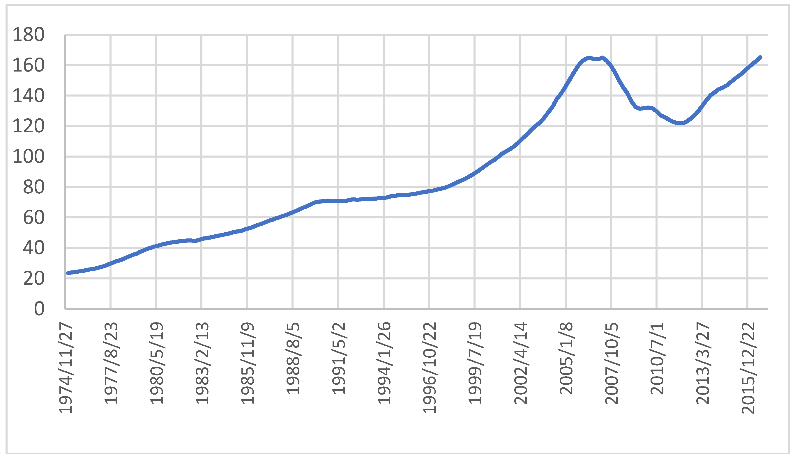
Before we began with the methodology, it was important to depict the performance of the housing and the financial wealth for the time period under investigation. Figure 1 reports the two national measures of house and financial wealth from 1975 to 2016. It seems that housing wealth never declined from 1975 to 2007. Even for the period where the DotCom crisis greatly impacted the financial wealth and consequently the economy (March 2000), housing wealth continued to rise across states.

3.2. Methodology

In this section we start our analysis by investigating if the variables are stationary. Based on two different methods, namely (a) the Im, Pesaran, and Shin W-stat, and (b) PP-Fisher chi-square we estimated the unit root hypothesis for consumption, income, financial wealth, and housing wealth. Tests assume a null hypothesis of joint stationarity against the null that all series are non-stationary. Under cross-sectional independence, each of these statistics were distributed as standard normal as both N (states) and T (time) increased.

Table 1. Results for panel unit root tests.

	Im, Pesaran and Shin		Phillips-Perron—Fisher Chi-Square
Variable	Constant	Constant Trend	Constant	Constant Trend
lnConsumption	−0.78(0.2179)	−6.42(0.0000)	138.05(0.0101)	202.79(0.0000)
lnIncome	0.29(0.6157)	2.67(0.9962)	82.73(0.9188)	59.72(0.9999)
lnFinancialWealth	8.65(1.0000)	−1.63(0.0511)	17.030(1.0000)	112.96(0.2154)
lnHousingWeatlh	2.46(0.9931)	−5.43(0.0000)	66.24(0.9977)	274.82(0.0000)
ΔlnConsumption	−24.26(0.0000)	−81.68(0.0000)	4194.05(0.0000)	5107.04(0.0000)
ΔlnIncome	−74.89(0.0000)	−77.48(0.0000)	4258.40(0.0000)	4089.47(0.0000)
ΔlnFinancialWealth	−88.25(0.0000)	−91.69(0.0000)	4748.11(0.0000)	4558.27(0.0000)
ΔlnHousingWeatlh	−83.54(0.0000)	−86.34(0.0000)	4527.15(0.0000)	4344.54(0.0000)

Ln is the natural log and Δ is the first difference operator. Numbers in parentheses are p-values. The maximum lag length is set to 6, determined by the Schwarz Bayesian Criterion.

presents the results of the panel unit root tests with intercept and intercept and trend. The analysis shows that all variables were stationary at the 5% significance level of the first difference, meaning that all variables were I (1) processes. Although the next step was to test for the long-run relationship and possible cointegration, we followed the CQS method—regressing the difference of consumption on the differences of income, financial, and housing wealth. While this specification addresses the non-stationarity issue, we understand that it does not take into account possible cointegration relationships. But we proceeded in order to compare our results with the ones obtained by CQS, Calomiris et al. [13,17], and Bampinas et al. [22].

The estimated equation is given as:

$$\Delta C_{it}={\beta }_1\Delta Y_{it}+{\beta }_2\Delta F{W}_{it}+{\beta }_3\Delta H{W}_{it}+FEffects+e_t$$

(1)

The equation shows the relationship between consumption (C), personal income (Y), stock (FW), and housing wealth (HW). We test three different specification models with the variables to be in first differences. Model I, II, and III are the basic specifications representing the effects of changes in both housing and stock-market wealth upon consumption. Model II explores further the nature of estimated wealth effects and their robustness by including state-specific time trends, while model III includes time fixed effects. Please note that the above model specifications, as articulated by Calomiris et al. [13], lead to inconsistent results, since the residual contains changes in permanent and current income, and these will likely be highly correlated with changes in housing and stock wealth. In order to correct for any correlation issues, we proceed with the estimation of three other models IV, V, and VI with the use of two-stage least squares and instrumental variables (The instrumental variables version takes account of possible endogeneity problems). As instruments we use lagged variables of income changes, housing wealth changes, and stock market changes. The hypothesis that the housing market wealth parameter is equal to the stock market wealth parameter was tested by the Wald test coefficient restriction.

As a next step we used the following error correction model (ECM) utilized by CQS. (Carrol et al. [26] argue that cointegration methods are problematic for estimating wealth effects, for at least two reasons. First, basic consumption theory does not imply the existence of a stable cointegrating vector; in particular, a change in the long-run growth rate or the long-run interest rate should change the relationship between consumption, income, and wealth. Second, even if changes to the cointegrating vector are ruled out by assumption, changes in any other feature of the economy relevant for the consumption/saving decision can generate such long-lasting dynamics that hundreds or thousands of years of data should be required to obtain reliable estimates of that vector; instead of ECM estimation, the literature suggests fixed-effect estimator procedure, dynamic Ordinary Least Square, mean group estimator, panel quantile regression, etc.). We understand that the basic format given by Brooks [27], as given by Equation (2), differs from the one presented by CQS, Equation (3), in a number of ways:

$$\Delta y_t={\beta }_1\Delta x_t+{\beta }_2\left(y_{t-1}-\gamma x_{t-1}\right)+error$$

(2)

$$\Delta C_t=\alpha \Delta C_{t-1}+{\beta }_1\Delta In{c}_t+{\beta }_2\Delta F{W}_t+{\beta }_3\Delta H{W}_t+\gamma [C_{t-1}-In{c}_{t-1}]+{\epsilon }_t$$

(3)

Firstly, CQS estimates Equation (3) by including lags of consumption, in order to correct for autocorrelation. Secondly, for the parameter γ, in Equation (2), which measures the speed of adjustment back to equilibrium and the long-term relationship between income and consumption, CQS impose without estimation—a cointegrating vector with a parameter of one.

Finally, given the original model (1), we are building the model for predicting consumption as follows. We construct our model in a time series for the U.S. and the eight states except the District of Columbia in order to use it for forecasting the consumption change. We forecast the consumption of Massachusetts, Illinois, Colorado, Nevada, California, Florida, New York, and the U.S. The equation specification consists of the dependent variable of consumption (in logs) followed by the list of regressors we used in this paper (the income and the two types of wealth). We included consumption with one lag as an independent variable for forecasting purposes (because the dependent variable is an auto-series). The estimated equation is:

$$\log C_t=\alpha \log C_{t-1}+{\beta }_1\log In{c}_t+{\beta }_2\log F{W}_t+{\beta }_3\log H{W}_t+{\epsilon }_t$$

(4)

We used the model to forecast future values of consumption which we have already estimated. In fact, we know the real values of consumption. Initially, we determined whether the forecast was accurate or not, which would then be compared with the actual values, and the difference between them. Therefore, we used the same set of data that was used to estimate the model’s parameters (in-sample forecasts) to see how well our model performs out-of-sample.

We first estimated the model using data from the 1986 fourth quarter to the 2016 first quarter. Then we conduct in-sample forecasts from the first quarter of 2005 until the first quarter of 2016, using a lagged dependent variable according the information criteria. We constructed dynamic forecasts to calculate multi-step forecasts starting from the first period in the forecast sample.

3.3. The Tax Reform Act of 1986

We took into consideration the Tax Reform Act enacted in October 1986 (TRA, 86). The TRA among others, encourages certain types of investments. It was a tax-simplification Act and chopped the top individual income tax rate from 50% to 28% while curbing special deductions, exclusions, and breaks, such as tax expenditures [28]. The Act also increased incentives favoring investment in owner-occupied housing, by increasing the home mortgage interest deduction. We proceed with re-estimating the model over the time period from 1986 to 2016. We understand that the two classes of wealth may have differences in terms of liquidity, with the housing to be less liquid since it is impossible to liquidate just a part of it. Furthermore, one should take into account the high processed fees for doing that. But since the end of 1986, home owners had the ability for home equity loans, refinancing with better terms, and thus, have more spending income for consumption.

3.4. The Case–Shiller Metropolitan areas Index

As a last step we performed the same analysis for the 10 metropolitan areas given by the Case–Shiller Composite 10 Index (the metropolitan areas are: Greater Boston, Chicago metropolitan area, Denver–Aurora Metropolitan Area, Las Vegas metropolitan area, Greater Los Angeles, South Florida metropolitan area, New York metropolitan area, San Diego County, San Francisco, and Washington Metropolitan Area). We first depict in Figure 2 the index from 1974 until the end of 2016 to see the evolution of the house prices over time. One could easily notice the positive trend displayed from 1974 until 2007. But the prevalent increase of the index occurred between 2002 and 2007, where ample market liquidity and lax credit conditions drove the house prices much higher, across the United States. From 2007 until the end of the 3rd quarter of 2011, house prices decrease significantly before start to increase again.

Testing the specific metropolitan areas comes from the notion that there might be distributional factors at work [11]. In other words, uneven distribution of wealth is very pronounced, and, although housing is held by a great majority of households, regardless of income classes, stock market wealth is held largely by a higher-income class. Indeed, this is more evident in other developed countries, but there is a notion that high-income class propensity to consume income and stock wealth is lower, pertaining that changes in housing wealth might have a larger effect on consumption. As Carroll [26] reports, the 20% of U.S. households hold most of the country’s overall net worth. Also, a good reason for testing the wealth effect on particular metropolitan areas, as CQS pointed out, is the fact that home prices have evolved very differently in different parts of the country, and therefore, there can be substantial differences in the elasticity of land supply, the performance of state economies, and their changing demographics.

Since there is no data available for the U.S. 10 metropolitan areas, we utilized the associated state-based data. For that reason, we tested the wealth effect on the consumption of the eight states where the metropolitan areas were part of them. In particular the states were Massachusetts, Illinois, Colorado, Nevada, California, Florida, New York, and District of Columbia.

4. Results and Discussion

Table 2. Consumption models in first differences. Panel data from 1975 to 2016.

Dependent Variable: Change in Consumption per Capita
	Ordinary Least Squares			Instrumental Variables
	I	II	III	IV	V	VI
Income	0.494 ***	0.489 ***	0.233 ***	0.209	0.156	0.378 ***
	(19.271)	(19.034)	(14.478)	(1.571)	(1.149)	(4.513)
Stock Market Wealth	0.058 ***	0.058 ***	0.029 ***	0.085 ***	0.081 ***	−0.010
	(9.364)	(9.413)	(5.662)	(3.716)	(3.553)	(0.227)
Housing Market Wealth	0.045 ***	0.045 ***	0.011 ***	0.070 ***	0.068 ***	0.018
	(7.670)	(7.624)	(3.381)	(3.177)	(3.048)	(1.603)
State Specific Time Trends	No	Yes	No	No	Yes	No
Quarterly Time Fixed Effects	No	No	Yes	No	No	Yes
R2	0.069	0.069	0.782	-	-	-
t-statistic	1.379	1.444	2.957	0.427	0.391	0.605
p-value for Ho	0.168	0.149	0.003	0.669	0.696	0.545

Note: Ho is the test of the hypothesis that the coefficient on housing market is equal to that of stock market; t-statistics are in parentheses and ***, are estimated values significant at the 1%, level.

depicts the results of all six models. The first observation is that consumption changes were significantly dependent on changes in income and in both forms of wealth. But in all specifications, stock market wealth had a positive and greater effect on consumption compared to the housing wealth effect. For models I and II, the stock market effect was 0.058, while for the housing effect the parameter was equal to 0.045. Both parameters appeared to be statistically significant at the 1% level. Interestingly enough, the sum of the financial and housing estimated parameters was almost equal to the sum obtained by CQS. Also, the estimated income effect on consumption is equal to around 0.49, which is within the 0.3–0.7 range found by Campbell and Mankiw [16].

The importance of the stock market wealth on consumption is reinforced by the results derived from model III, which includes fixed effects, and by models IV and V, where changes in stock market wealth have still greater impact than the housing effect on changes in consumption. The results are in direct contrast to the findings of CQS, but in an agreement with Calomiris et al. [13]. Also, Table 2 reports the t-statistics for the hypothesis that the coefficient of stock market wealth is equal to the coefficient of the housing market wealth. The results suggest that we could not reject the hypothesis that financial wealth could be equal in importance to housing wealth. Only in model III, was financial wealth greater and more important than housing wealth.

Table 3. Error correction consumption models. Panel data from 1975 to 2016.

Dependent Variable: Change in Consumption per Capita
	I	II	III
Change in Income	0.499 ***	0.495 ***	0.264 ***
	(23.729)	(23.647)	(15.710)
Change in Stock Market Wealth	0.060 ***	0.059 ***	0.024 ***
	(12.370)	(12.354)	(4.775)
Change in Housing Market Wealth	0.047 ***	0.047 ***	0.012 ***
	(10.175)	(10.092)	(3.592)
Lagged Change in Consumption (1 to 8)	0.215 ***	0.216 ***	0.076 ***
	(20.783)	(20.953)	(6.766)
Lagged Ratio of Consumption to Income	−0.015 ***	−0.031 ***	−0.017 ***
	(8.191)	(11.472)	(9.969)
State Specific Time Trends	No	Yes	No
Quarterly Timed Fixed Effects	No	No	Yes
R2	0.455	0.459	0.791
t-statistic	1.802	1.846	2.071
p-value for Ho	0.071 *	0.065 *	0.038 **

Note: Ho is the test of the hypothesis that the coefficient on the housing market is equal to that of the stock market; t-statistics are in parentheses and ***, **, and * are estimated values significant at the 1%, 5%, and 10% level, respectively.

presents the results of the error correction model and supports the highly significant immediate effect of financial wealth on consumption, as well as the housing effect. But the financial wealth coefficient is larger in magnitude than the housing coefficient. For models I and II, the financial coefficient took a value of around 0.062, while the housing parameter was 0.047. In the third model, when fixed effects were included, the estimated parameters decreased in magnitude but still financial wealth appeared to be greater and more significant than the housing wealth effect. Furthermore, the results obtained by ECM were consistent with the results found by the first difference model specification. As for the lagged ratio of consumption to income, the coefficient was negative and significant in both cases, revealing an immediate correction of the potential shocks. It also suggests that transitory shocks, arising from changes in other variables in the model or in the error term, will have an immediate effect on consumption. This effect will eventually be offset, unless the shock is ultimately confirmed by income changes [4].

In

Table 4. Error Correction Consumption Models for the period 1987-2016, after the introduction of the Tax Reform Act in 1986.

Dependent Variable: Change in Consumption per Capita
	I	II	III
Change in Income	0.532 ***	0.528 ***	0.425 ***
	(19.093)	(19.025)	(17.376)
Change in Stock Market Wealth	0.068 ***	0.066 ***	0.010 **
	(13.257)	(12.952)	(1.748)
Change in Housing Market Wealth	0.042 ***	0.042 ***	0.009 ***
	(8.331)	(8.361)	(2.857)
Lagged Change in Consumption (1 to 8)	0.208 ***	0.211 ***	0.042 ***
	(17.249)	(17.562)	(3.219)
Lagged Ratio of Consumption to Income	−0.035 ***	−0.057 ***	−0.037 ***
	(11.362)	(13.753)	(12.754)
State Specific Time Trends	No	Yes	No
Quarterly Time Fixed Effects	No	No	Yes
R2	0.313	0.321	0.713
t-statistics	15.768	15.798	6.156
p-value for Ho	0.000	0.000	0.000

Note: Ho is the test of the hypothesis that the coefficient on the housing market is equal to that of the stock market; t-statistics are in parentheses and *** and**, are estimated values significant at the 1% and 5%, level, respectively.

we repeat the same methodology and present only the estimates of the error correction models, with the sample data spanning from end 1986 until 2016. The results support again the highly significant immediate effect of financial wealth on consumption, which is more than 2 cents higher than the effect of housing wealth. Surprisingly, we find that the housing effect is lower than before, irrespective of the estimation method chosen. The opposite is reported for the financial wealth where the effect on consumption is now 0.066 to 0.068 instead of 0.060. It is worth pointing out the increase, in absolute terms, of the estimated parameter measuring the lagged ratio of consumption to income, reviling again a very immediate correction of the any potential shocks. In concluding, based on the error correction estimates the 1986 Act seems not to change people preferences and still the financial wealth effect is greater and significantly more important, based on the Wald test, than the housing wealth effect on consumption.

Table 5. Ordinary Least Square model for consumption and error correction for the period 1987–2016 for the eight states after the introduction of the Tax Reform Act in 1986.

Dependent Variable: Change in Consumption per Capita
	Ordinary Least Squares			Error Correction Model
	I	II	III	IV	V	VI
Change in Income	0.583 ***	0.589 ***	0.549 ***	0.599 ***	0.594 ***	0.605 ***
	(6.131)	(6.189)	(5.832)	(6.565)	(6.517)	(6.062)
Change in Stock Market Wealth	0.021	0.022	0.004	0.030 *	0.029*	0.002
	(1.225)	(1.278)	(0.272)	(1.862)	(1.820)	(0.132)
Change in Housing Market Wealth	0.052 ***	0.051 ***	0.022 *	0.055 ***	0.055 ***	0.024 **
	(3.203)	(3.183)	(1.873)	(3.748)	(3.747)	(2.018)
Lagged Change in Consumption (1 to 8 lags)	-	-	-	0.205 ***	0.207 ***	0.103 ***
				(6.525)	(6.613)	(2.884)
Lagged Ratio of Consumption to Income	-	-	-	−0.032 ***	−0.044 ***	−0.029 ***
				(4.888)	(5.051)	(4.410)
State Specific Time Trends	No	Yes	No	No	Yes	No
Quarterly Time Fixed Effects	No	No	Yes	No	No	Yes
R2	0.061	0.063	0.681	0.269	0.272	0.688
t-statistic	1.261	1.210	0.873	1.122	1.151	1.063
p-value for Ho	0.208	0.227	0.383	0.262	0.250	0.288

Note: Ho is the test of the hypothesis that the coefficient on the housing market is equal to that of the stock market; t-statistics are in parentheses and ***, **, and * are estimated value significant at the 1%, 5%, and 10% level, respectively.

presents the results of the first three specification models, where the variables are in first differences, along with the error correction models, in an attempt to test the consistency of the estimated parameters. The results are surprisingly different now and in direct contrast to the findings of the previous sections of the paper. Now, the estimated housing effect is larger in magnitude and more significant than the financial wealth effect. The MPC out of housing wealth is in the region of 0.052 while the MPC for stock wealth is around 0.021. In most of the cases, the stock wealth estimate was not even statistically significant. In addition, the estimated income coefficient was much greater in magnitude and steadily in the area of 0.59 compared with only 0.49 before, and still within the 0.3–0.7 range estimated by Cambell and Mankiw [16]. The results from the first three models were supported by the error correction estimates depicted by the models IV, V, and VI in Table 5. The estimates of the housing wealth parameter were more than double in magnitude than the estimates of the stock market wealth. The coefficient of lagged ratio of consumption to income was once more very small, indicating the immediate restoration of consumption after a shock in the residuals in the short run.

Forecasting the Consumption Change

Table 6. Forecast evaluation table.

The Forecast Statistics for the 7 States Comprised of the Case–Shiller Index and the U.S.
States	Root Mean Square Error	Mean Absolute Error	Theil Inequality Coefficient	Bias Variance	Variance Proportion
Massachusetts	0.0344	0.0233	0.0018	0.3492	0.1775
Ilinois	0.0366	0.0277	0.0019	0.0234	0.1433
Colorado	0.0321	0.0261	0.0017	0.4354	0.0724
Nevada	0.0751	0.0558	0.0039	0.0193	0.5268
California	0.0339	0.0268	0.0017	0.2390	0.0000
Florida	0.0473	0.0419	0.0025	0.0656	0.2353
New York	0.0452	0.0344	0.0023	0.0235	0.3121
USA	0.0262	0.0213	0.0014	0.0011	0.0132

compares the forecasted (predicted) values from the model (over the period 2005 q1 to 2016 q1) to the actual data and computes the forecast evaluation, see Table 6.

The root mean squared error was about 0.02–0.07 and the mean absolute error ranged from 0.02–0.04. Bias proportion was about 0.00–0.43, while the variance proportion was about 0.01–0.31.

The reported forecast statistics indicated that our forecasting model perform well out-of-sample.

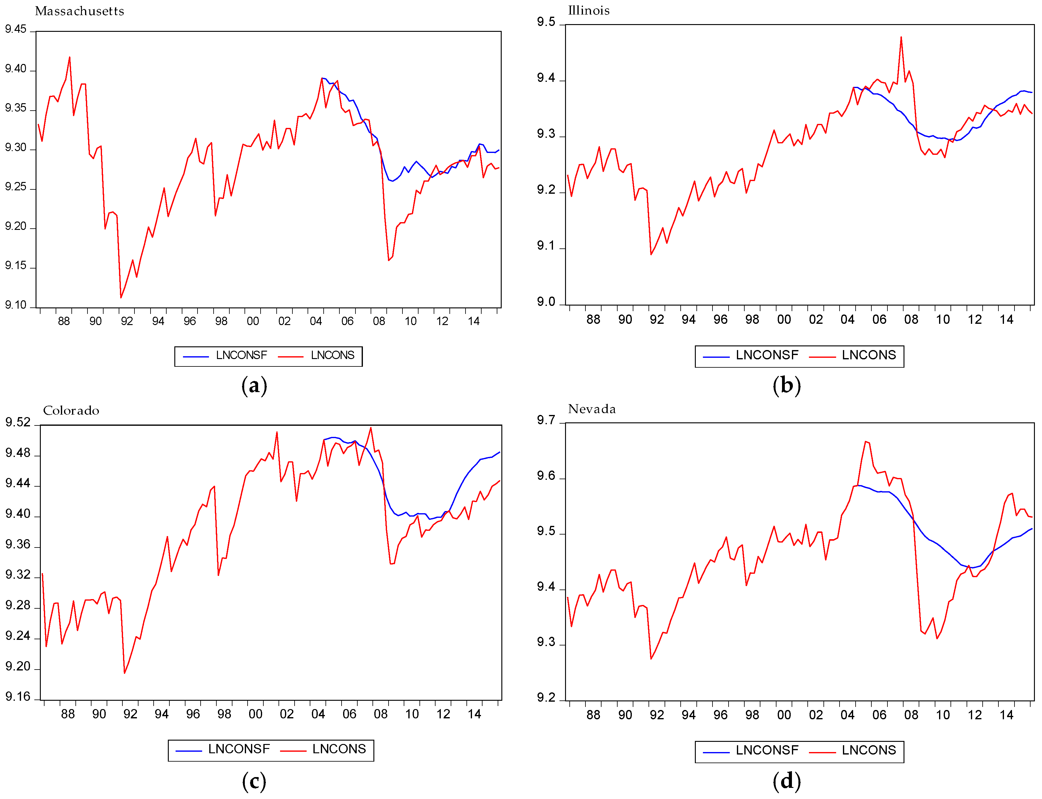
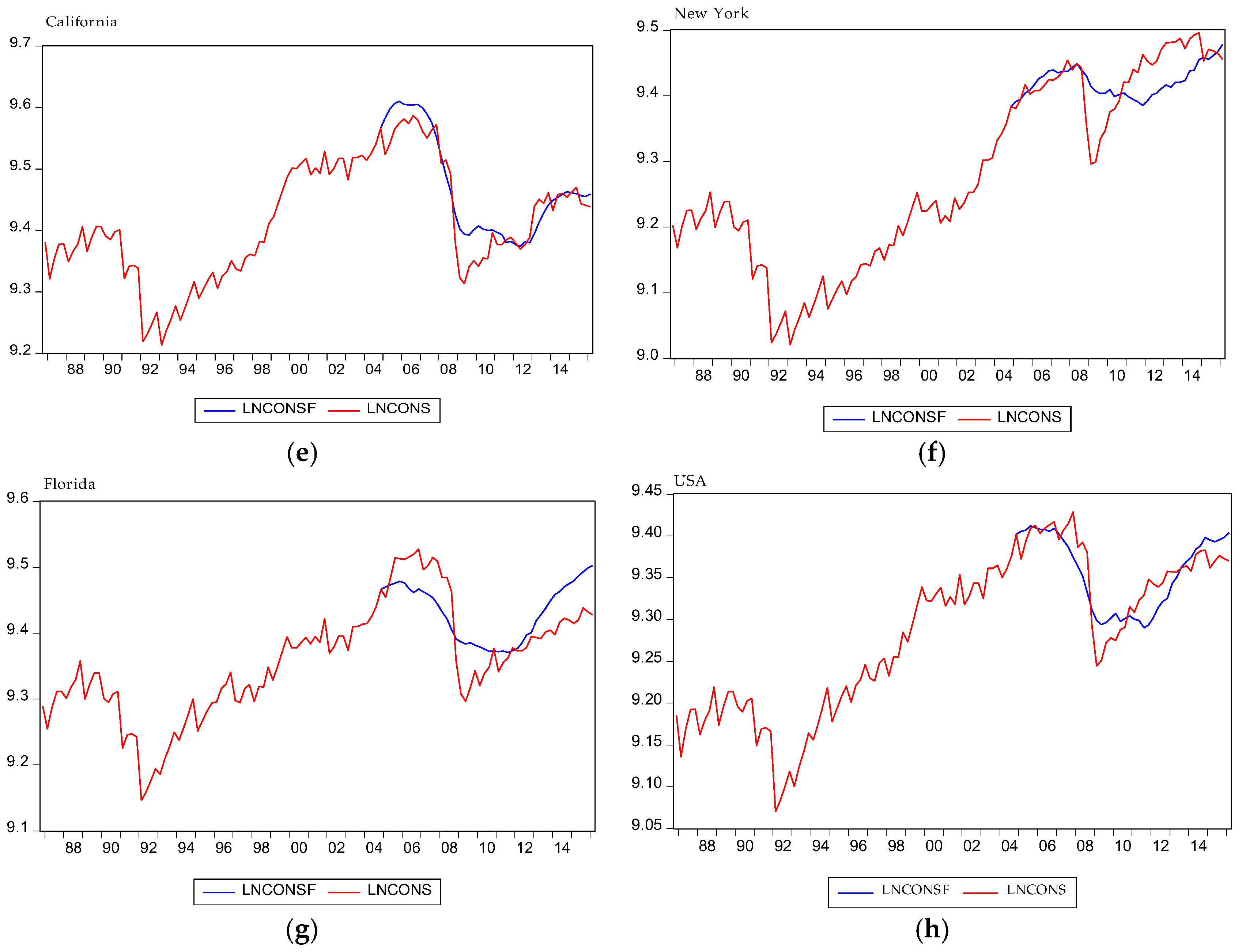
Figure 3 display the results of forecasting consumption changes in Massachusetts, Illinois, Colorado, Nevada, California, Florida, New York, and the U.S.

We conclude that the big dip in consumption in 2008 was not predicted in any state, as well as the large rise in consumption for 2005. Generally, extreme consumption behaviors were not predictable. Our panel results show that the effect of housing wealth is larger on consumption compared to financial wealth. Simultaneously, literature evidence [12] finds that the relationship between house prices and consumption is stronger for younger than older households. The young are more vulnerable in irrational behaviors and more likely to be credit-constrained, and thus, willing to borrow against any increase in housing equity.

Furthermore, while the forecast showed a recession from 2008 to the last quarter of 2011, in fact, from the first quarter of 2009 the economy in America began to recover in all states, probably due to quantitative easing, which was started in November 2008. The Federal Reserve increased the amount of money by going to the financial markets to buy assets and generating new money to pay for it. Specially, in New York and Nevada the real consumption exceeded forecasts.

5. Conclusions

We have followed Case et al. [4] in an attempt to estimate the effect of changes in financial and housing wealth on changes in household consumption for the time period between 1975 to 2016. Constructing the housing and finance data differently from the method used by Case et al. [4], we find first that both financial and housing wealth were significant determinants of household consumption and secondly the effect of financial wealth was larger in magnitude from the housing wealth effect. For most of model specifications, a $1 change in stock market wealth will change consumption by 5.8–6 cents, whereas in terms of housing wealth consumption, it will increase by only 4.5–4.7 cents. Our panel results are in contrast to CQS studies and in line with the ones obtained by Calomiris et al. [13]. But when we tested the top 10 metropolitan areas due to the fact that distributional factors could be at work and the that home prices have evolved very differently in different parts of the country, meaning substantial differences in the elasticity of land supply, we found that the estimate housing wealth had greater and more robust effects on consumption than the stock market wealth. The difference with the CQS results could be explained because we mainly used an alternative methodology for measuring of stock market and housing wealth. Therefore, we could agree with Calomiris et al. [17] that the results were very sensitive with the choice of housing wealth measure.

Finally, we forecasted consumption change in the seven states that included the 10 (richer) Metropolitan areas comprised of the well-known Case–Shiller 10 City Composite Index and the U.S. We concluded that our model was a good predictor and extreme behaviors in consumption were not predictable. Additionally, while the forecast showed a recession from 2008 to the last quarter of 2011, in fact from the first quarter of 2009 the economy in America began to recover. The main reason may be the aggressive monetary policy followed and the quantitative easing that spurred consumption. However, expectations for greater consumption were not verified for most areas.