
Hybrid Energy-Powered Electrochemical Direct Ocean Capture Model


Abstract
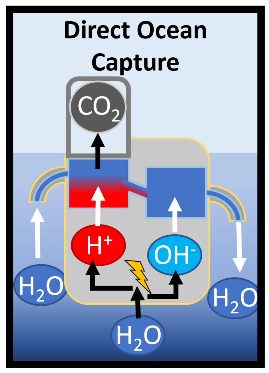
1. Introduction
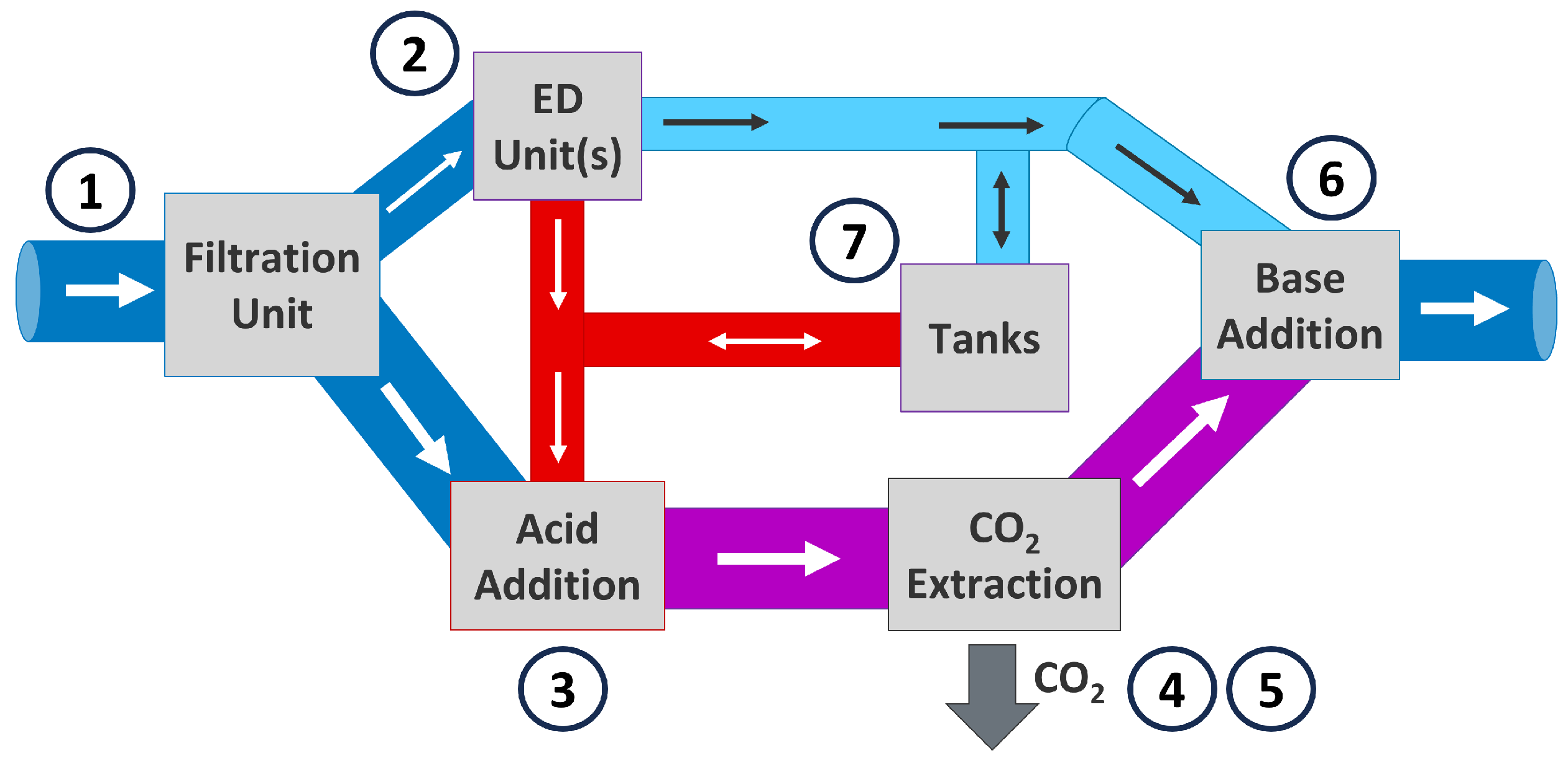
2. Materials and Methods
2.1. Electrochemical Model
2.2. Ocean Chemistry Model
2.2.1. Acid Addition and Extraction
2.2.2. Base Addition and Seawater Neutralization
2.3. Pumps and Vacuum
2.3.1. Liquid Pump Equations
2.3.2. Gas Vacuum Equations
2.4. Post-Processing
2.4.1. Purification
2.4.2. Compression
2.5. Model Operation Scenarios
2.5.1. Scenario 1: ED Units Used for DOC, Tanks Are Full
2.5.2. Scenario 2: ED Units Used for DOC and Filling Tanks
2.5.3. Scenario 3: Solutions in Tank Used for DOC
2.5.4. Scenario 4: ED Units Just Fill Tanks, No DOC Is Performed
2.6. DOC Model Assumptions
2.7. Hybrid Energy Models and Parameters
2.8. Comparison with Industry Parameters
2.9. Characteristics of Example Simulations
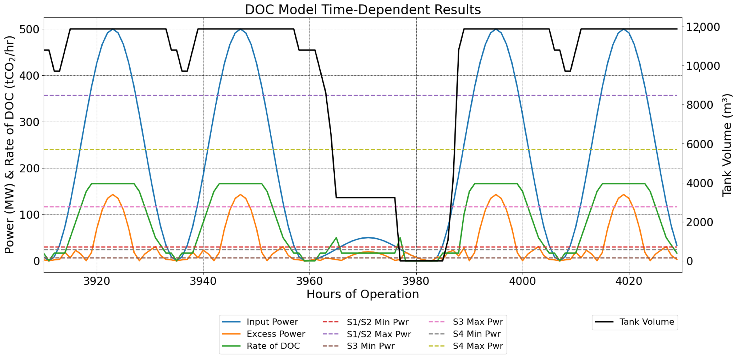
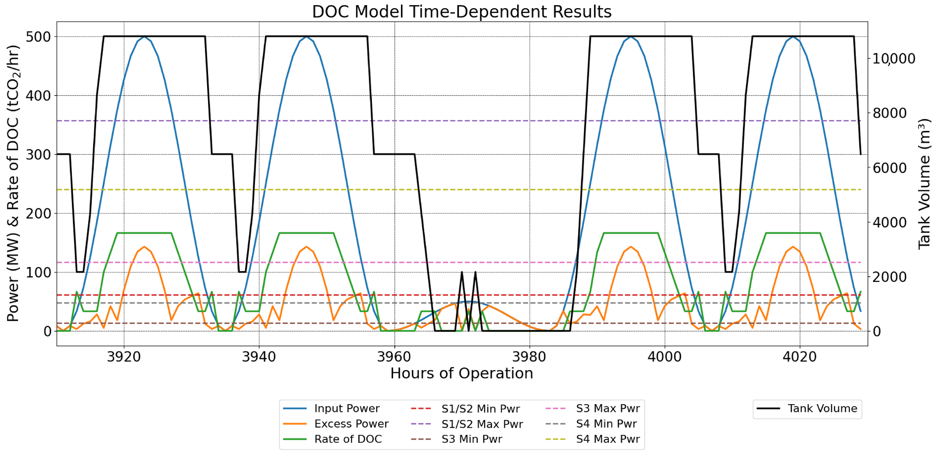
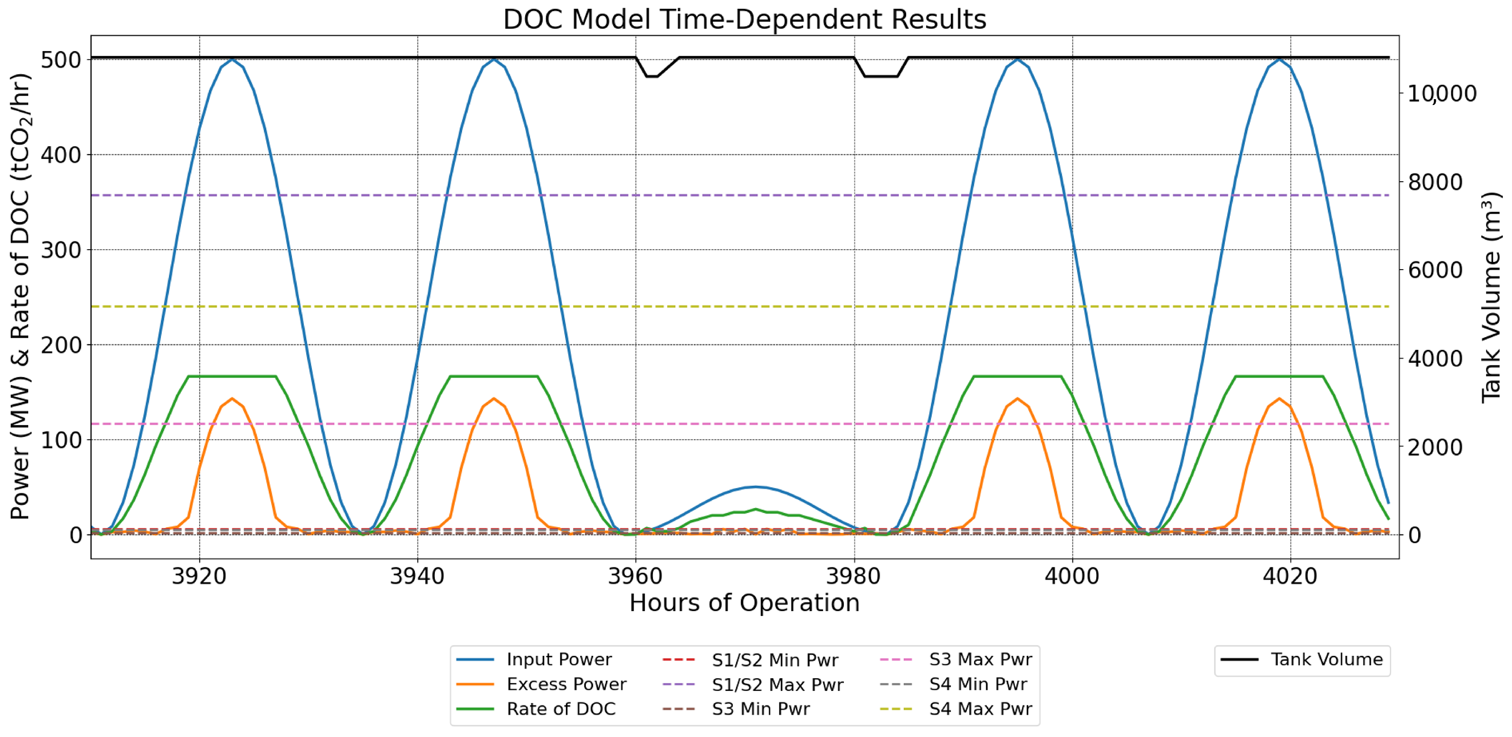
2.9.1. Sine-Wave Power Profile with Periods of Lower Power
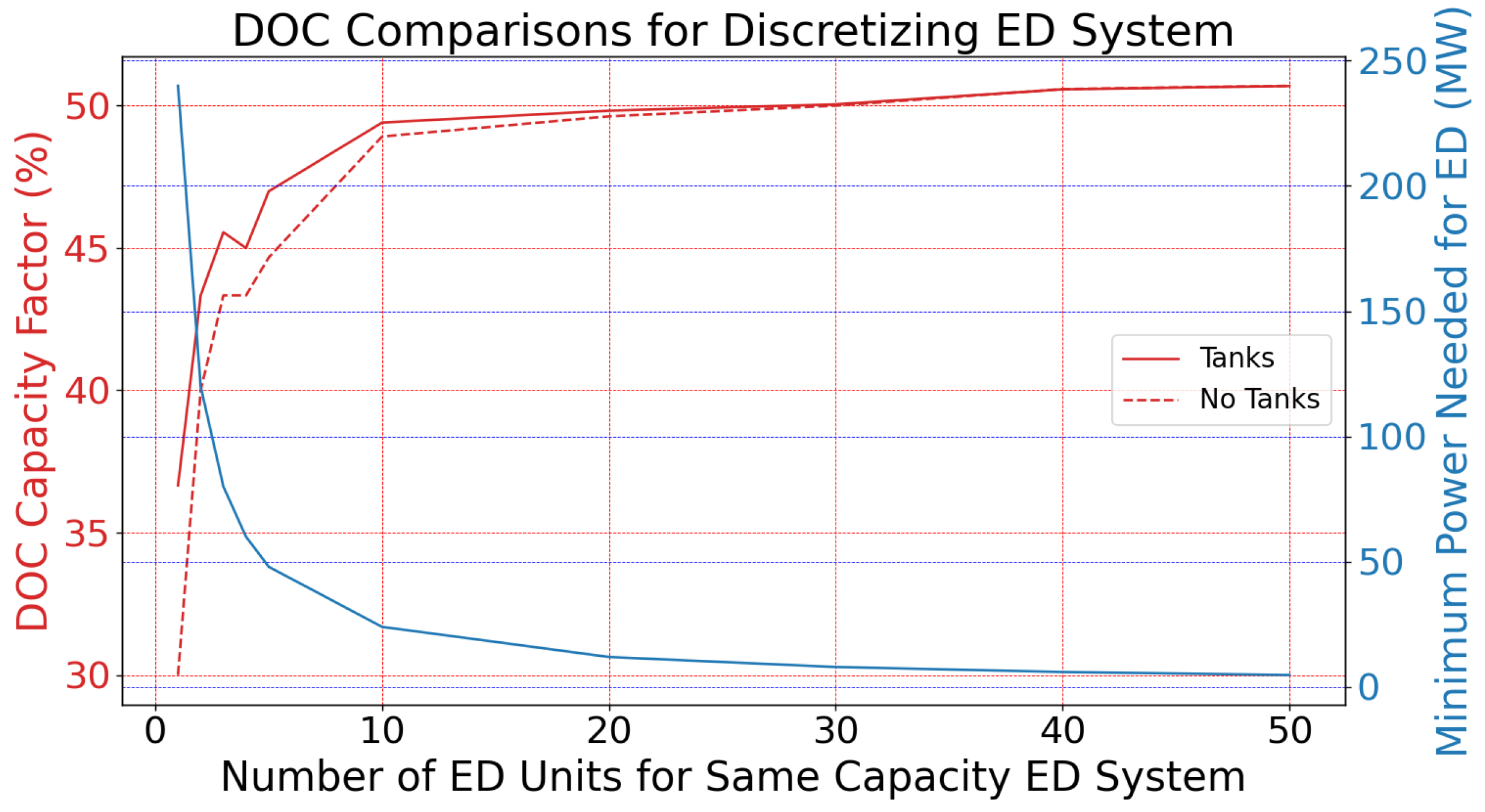
2.9.2. Effect of ED Discretization Under Sine-Wave Power Profile
2.9.3. Case Studies with Hybrid Renewable Energy Systems
3. Results
3.1. Comparison with Industry Parameters
3.2. Sine-Wave Power Profile with Periods of Lower Power
3.3. Effect of ED Discretization Under Sine-Wave Power Profile
3.4. Case Studies with Hybrid Renewable Energy Systems
4. Discussion
5. Conclusions
Author Contributions
Funding
Institutional Review Board Statement
Informed Consent Statement
Data Availability Statement
Acknowledgments
Conflicts of Interest
Abbreviations
| CDR | Carbon dioxide removal | MW | Megawatt |
| Carbon dioxide | MWh | Megawatt-hour | |
| DOC | Direct ocean capture | NREL | National Renewable Energy Laboratory |
| ED | Electrodialysis | ppt | Parts per thousand |
| H2I | H2Integrate | PSA | Pressure swing absorption |
| hr | Hour | S | Scenario |
| J | Joule | t | Metric tons of carbon dioxide |
| kWh | Kilowatt-hour | U.S. | United States |
| LCOE | Levelized cost of energy | USD | United States dollar |
| mCDR | Marine carbon dioxide removal | yr | Year |
Constants and Variables
| Concentration of dissolved in seawater after acid addition (in mol/m3) | |
| Concentration of dissolved in seawater after extraction (in mol/m3) | |
| Initial concentration of DIC in seawater (in mol/m3) | |
| Concentration of DIC in seawater remaining after extraction (in mol/m3) | |
| Acid concentration in seawater after acid addition (in mol/m3) | |
| Acid concentration in seawater after extraction and before base addition | |
| (in mol/m3) | |
| Acid concentration in seawater after base addition (in mol/m3) | |
| Acid concentration in seawater at second equivalence point (in mol/m3) | |
| Concentration of TA in seawater after acid addition (in mol/m3) | |
| Concentration of TA in seawater after extraction (in mol/m3) | |
| Concentration of TA in seawater after base addition (in mol/m3) | |
| Initial concentration of TA in seawater (in mol/m3) | |
| Concentration of acid generated by ED system (in mol/m3) | |
| Concentration of acid generated by a single ED unit (in mol/m3) | |
| Concentration of base generated by ED system (in mol/m3) | |
| Concentration of base generated by a single ED unit (in mol/m3) | |
| Initial concentration of acid in seawater before the DOC process (in mol/m3) | |
| Initial concentration of base in seawater before the DOC process (in mol/m3) | |
| First stoichiometric equilibrium constant for carbonate buffer solution | |
| Second stoichiometric equilibrium constant for carbonate buffer solution | |
| Water dissociation constant of seawater | |
| Mass rate of extracted from seawater (in t/hr) | |
| Mole rate of acid added to seawater (mol/s) | |
| Mole rate of extracted from seawater (in mol/s) | |
| Mole rate of dissolved in seawater (in mol/s) | |
| Mole rate of TA in seawater after acid addition (mol/s) | |
| Mole rate of TA in seawater initially (mol/s) | |
| Mole rate of gas mixture moving through the vacuum (mol/s) | |
| Maximum number of ED units that can be used by the ED system | |
| Minimum number of ED units that can be used by the ED system | |
| Total number of cases in a given scenario | |
| Number of active ED units at a given time-step | |
| Number of active ED units being used for DOC at a given time-step | |
| Number of active ED units being used for filling the tanks at a given time-step | |
| Atmospheric pressure (in bar) | |
| Power needed by ED system at a given time-step (in W) | |
| Power required by a single ED unit (in W) | |
| Initial pH of seawater | |
| Flow rate of acid out of ED system at a given time-step (in m3/s) | |
| Flow rate of acid out of a single ED unit (in m3/s) | |
| Flow rate of acid needed to consume the moles of total alkalinity (in m3/s) | |
| Flow rate of acid remaining after all moles of total alkalinity are consumed (in m3/s) | |
| Flow rate of acid used for DOC (in m3/s) | |
| Flow rate of acidified seawater (in m3/s) | |
| Flow rate of acid moving to and from the tanks (in m3/s) | |
| Flow rate of base out of ED system at a given time-step (in m3/s) | |
| Flow rate of base out of a single ED unit (in m3/s) | |
| Flow rate of base used for DOC (in m3/s) | |
| Flow rate of base moving to and from the tanks (in m3/s) | |
| Flow rate of seawater into ED system at a given time-step (in m3/s) | |
| Flow rate of seawater into a single ED unit (in m3/s) | |
| Flow rate of effluent seawater (in m3/s) | |
| Flow rate of seawater remaining after portion is used for ED system (in m3/s) | |
| Intake flow rate of seawater at a given time-step (in m3/s) | |
| Average flow rate of gas moving through vacuum (in m3/s) | |
| R | Universal gas constant (in J/molK) |
| S | Salinity of seawater (in ppt) |
| Temperature of seawater (in Kelvin) | |
| Temperature of air (in Kelvin) | |
| Hours of minimum DOC that can be provided by the tanks | |
| Maximum volume of the acid tanks (in m3) | |
| Maximum volume of the base tanks (in m3) | |
| Energy required to separate from a mixed gas stream (in J/mol) | |
| Minimum energy required to separate from a mixed gas stream (in J/mol) | |
| Purity or mole fraction of | |
| Fraction of extracted from seawater | |
| Efficiency of the pumps | |
| Fraction of intake seawater used by ED system | |
| Efficiency of vacuum | |
| Pressure drop for pumps and vacuum (in bar) | |
| ED unit’s efficiency in producing acid (in Wh/mol HCl) | |
| ED unit’s efficiency in producing base (in Wh/mol NaOH) | |
| Efficiency for purification |
Appendix A. Temperature and Salinity Dependence
Appendix A.1. Temperature and Salinity Impacts on Ocean Chemistry
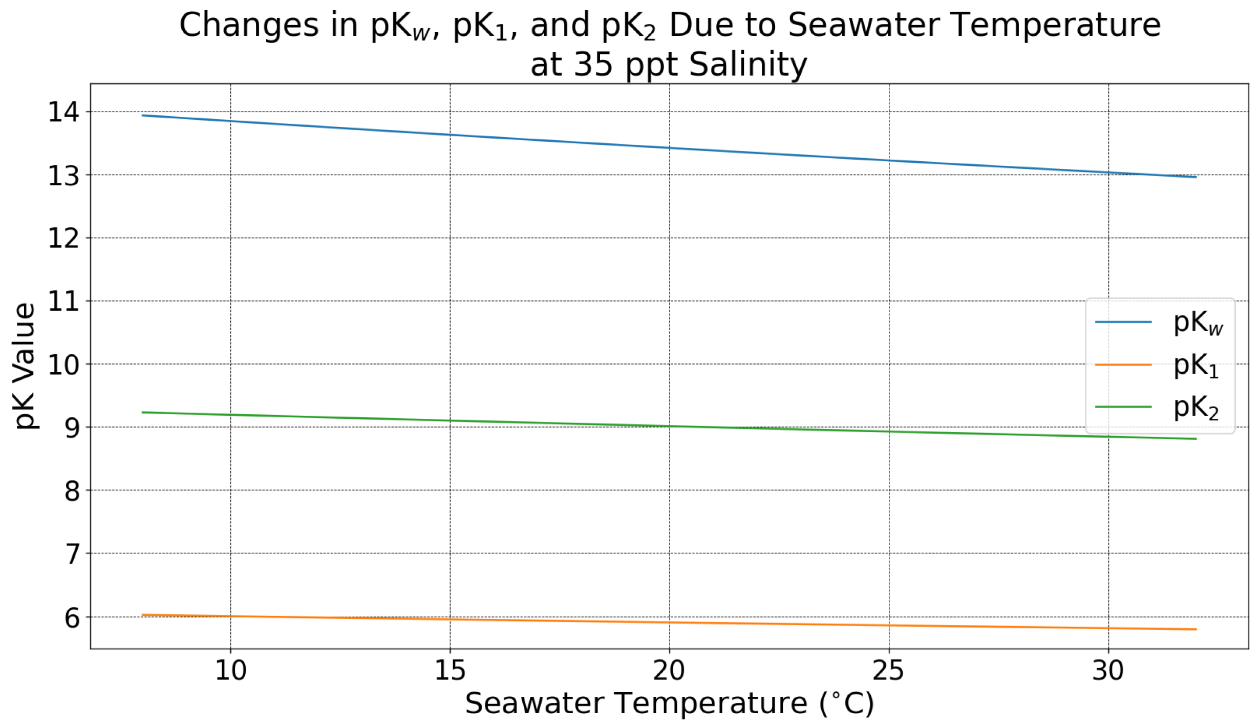
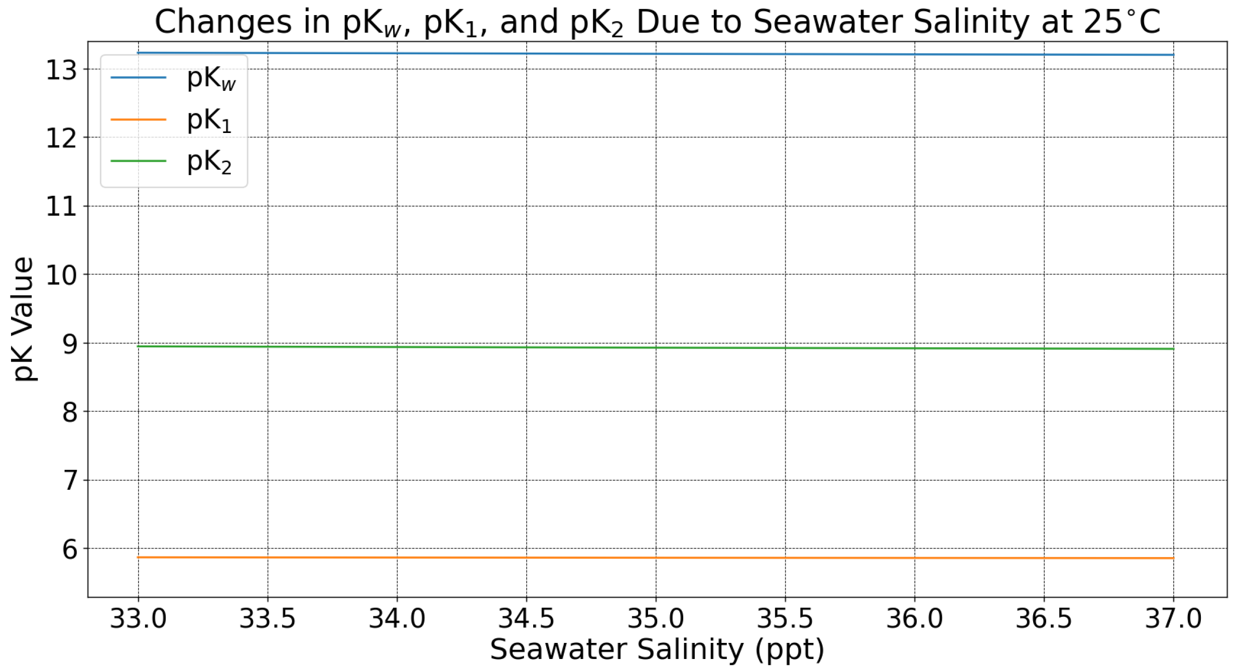
Appendix A.2. Effect of Seawater Temperature and Salinity on DOC and pH Effluent: Methods
Appendix A.3. Effect of Seawater Temperature and Salinity on DOC and pH Effluent: Results

References
- Patterson, B.; Mo, F.; Borgschulte, A.; Hillestad, M.; Joos, F.; Kristiansen, T.; Sunde, S.; van Bokhoven, J. Renewable CO2 recycling and synthetic fuel production in a marine environment. Proc. Natl. Acad. Sci. USA 2019, 116, 12212–12219. [Google Scholar] [CrossRef] [PubMed]
- Niffenegger, J.; Greene, D.; Thresher, R.; Lawson, M. Mission Analysis for Marine Renewable Energy to Provide Power for Marine Carbon Dioxide Removal; Technical Report; National Renewable Energy Laboratory: Golden, CO, USA, 2023.
- Doney, S.; Buck, H.; Buesseler, K.; Iglesias-Rodriguez, M.; Moran, K.; Oschlies, A.; Renforth, P.; Roman, J.; Sant, G.; D.A, S.; et al. A Research Strategy for Ocean-Based Carbon Dioxide Removal and Sequestration; Technical Report; National Academies of Sciences, Engineering, and Medicine: Washington, DC, USA, 2022. [Google Scholar]
- Eisaman, M.; Rivest, J.; Karnitz, S.; de Lannoy, C.; Jose, A.; DeVaul, R.; Hannun, K. Indirect ocean capture of atmospheric CO2: Part II. Understanding the cost of negative emissions. Int. J. Greenh. Gas Control 2018, 70, 254–261. [Google Scholar] [CrossRef]
- de Lannoy, C.; Eisaman, M.; Jose, A.; Karntiz, S.; DeVaul, R.; Hannun, K.; Rivest, J. Indirect ocean capture of atmospheric CO2: Part I. Prototype of a negative emissions technology. Int. J. Greenh. Gas Control 2018, 70, 243–253. [Google Scholar] [CrossRef]
- Digdaya, I.; Sulliva, I.; Lin, M.; Han, L.; Cheng, W.; Atwater, H.; Xiang, C. A direct coupled electrochemical system for capture and conversion of CO2 from oceanwater. Nat. Commun. 2020, 11, 4412. [Google Scholar] [CrossRef] [PubMed]
- Captura. Equinor and Captura Partner to Develop Ocean Carbon Removal. Available online: https://capturacorp.com/equinor-and-captura-partner-to-develop-ocean-carbon-removal/ (accessed on 28 March 2024).
- Captura. The First Wave of Climate Solutions. Available online: https://capturacorp.com/technology/ (accessed on 11 July 2024).
- He, W.; LeHenaff, A.; Amrose, S.; Buonassisi, T.; Peters, I. Voltage- and flow-controlled electrodialysis batch operation: Flexible and optimized brackish water desalination. Desalination 2021, 500, 114837. [Google Scholar] [CrossRef]
- Mir, N.; Bicer, Y. Integration of electrodialysis with renewable energy sources for sustainable freshwater production: A review. J. Environ. Manag. 2021, 289, 112496. [Google Scholar] [CrossRef] [PubMed]
- He, W.; LeHenaff, A.; Amrose, S.; Buonassisi, T.; Peters, I.; Winters, A. Flexible batch electrodialysis for low-cost solar-powered brakish water desalination. Nat. Water 2024, 2, 370–379. [Google Scholar] [CrossRef]
- Wang, H.; Pilcher, D.; Kearney, K.; Cross, J.; Shugart, O.; Eisaman, M.; Carter, B. Simulated Impact of Ocean Alkalinity Enhancement on Atmospheric CO2 Removal in the Bering Sea. Earth’s Future 2022, 11, e2022EF002816. [Google Scholar] [CrossRef]
- National Renewable Energy Laboratory. H2Integrate. 2025. Available online: https://github.com/NREL/H2Integrate (accessed on 25 September 2024).
- Culcasi, A.; Gurreri, L.; Cipollina, A.; Tamburini, A.; Micale, G. A comprehensive multi-scale model for bipolar membrane electrodialysis (BMED). Chem. Eng. J. 2022, 437, 135317. [Google Scholar] [CrossRef]
- Captura. Carbon Dioxide Removal Pathway: Ocean Health and MRV; Technical Report; Captura Corp.: Pasadena, CA, USA, 2023. [Google Scholar]
- Socolow, R.; Desmond, M.; Aines, R.; Blackstock, J.; Bolland, O.; Kaarsberg, T.; Lewis, N.; Mazzotti, M.; Pfeffer, A.; Sawyer, K.; et al. Direct Air Capture of CO2 with Chemicals: A Technology Assessment for the APS Panel on Public Affairs; Technical Report; The American Physical Society: College Park, MD, USA, 2011. [Google Scholar]
- House, K.; Baclig, A.; Ranjan, M.; vanNierop, E.; Wilcox, J.; Herzog, H. Economic and energetic analysis of capturing CO2 from ambient air. Proc. Natl. Acad. Sci. USA 2011, 108, 20428–20433. [Google Scholar] [CrossRef] [PubMed]
- Wilcox, J.; Haghpanah, R.; Rupp, E.; He, J.; Lee, K. Advancing Adsorption and Membrane Separation Processes for the Gigaton Carbon Capture Challenge. Annu. Rev. Chem. Biomol. Eng. 2014, 5, 479–505. [Google Scholar] [CrossRef] [PubMed]
- Ogden, J. Hydrogen Energy Systems Studies; Technical Report; Princeton University: Princeton, NJ, USA, 1999. [Google Scholar]
- Ansolabehere, S.; Beer, J.; Deutch, J.; Ellerman, A.; Friedman, S.; Herzog, H.; Jacoby, H.; Joskow, P.; McRae, G.; Lester, R.; et al. The Future of Coal: Options for a Carbon-Constrained World; Technical Report; Massachusetts Institute of Technology: Cambridge, MA, USA, 2007. [Google Scholar]
- Jackson, S.; Brodal, E. A comparison of the energy consumption for CO2 compression process alternatives. In Proceedings of the 8th International Conference on Environment Science and Engineering (ICESE 2018), Barcelona, Spain, 11–13 March 2018; pp. 1–14. [Google Scholar] [CrossRef]
- Humphreys, M.; Lewis, E.; Sharp, J.; Pierrot, D. PyCO2SYS v1.8: Marine carbonate system calculations in Python. Geosci. Model Dev. 2022, 15, 15–43. [Google Scholar] [CrossRef]
- National Renewable Energy Laboratory. ProFAST (Production Financial Analysis Scenario Tool). 2023. Available online: https://github.com/NREL/ProFAST (accessed on 20 September 2023).
- Gaertner, E.; Rinker, J.; Sethuraman, L.; Zahle, F.; Anderson, B.; Barter, G.; Abbas, N.; Meng, F.; Bortolotti, P.; Skrzypinski, W.; et al. Definition of the IEA 15-Megawatt Offshore Reference Wind Turbine; Technical Report; International Energy Agency: Paris, France, 2020. [Google Scholar]
- National Renewable Energy Laboratory. FLORIS: FLOw Redirection and Induction in Steady State. 2023. Available online: https://www.nrel.gov/wind/floris.html (accessed on 25 September 2023).
- National Renewable Energy Laboratory. Wind Integration National Dataset Toolkit. 2023. Available online: https://www.nrel.gov/grid/wind-toolkit.html (accessed on 20 May 2023).
- National Renewable Energy Laboratory. 2024 Annual Technology Baseline. 2024. Available online: https://atb.nrel.gov/ (accessed on 15 May 2024).
- Neary, V.S.; Previsic, M.; Jepsen, R.A.; Lawson, M.J.; Yu, Y.H.; Copping, A.E.; Fontaine, A.A.; Hallett, K.C.; Murray, D.K. Methodology for Design and Economic Analysis of Marine Energy Conversion (MEC) Technologies. In Proceedings of the 2nd Marine Energy Technology Symposium (METS 2014), Seattle, WA, USA, 15–18 April 2014; pp. 1–6. [Google Scholar]
- National Renewable Energy Laboratory. PySAM. Available online: https://github.com/nrel/pysam (accessed on 20 May 2023).
- National Renewable Energy Laboratory. Hindcast Data Downloads API|NREL: Developer Network. Available online: https://developer.nrel.gov/docs/wave/hindcast/ (accessed on 28 September 2024).
- Musial, W.; Heimiller, D.; Beiter, P.; Scott, G.; Draxl, C. 2016 Offshore Wind Energy Resource Assessment for the United States; Technical Report; National Renewable Energy Laboratory: Golden, CO, USA, 2016.
- Kilcher, L.; Fogarty, M.; Lawson, M. Marine Energy in the United States: An Overview of Opportunities; Technical Report; National Renewable Energy Laboratory: Golden, CO, USA, 2021.
- NREL. Marine Energy Atlas. Available online: https://maps.nrel.gov/marine-energy-atlas/ (accessed on 25 September 2024).
- Bolson, N.; Prieto, P.; Patzek, T. Capacity factors for electrical power generation from renewable and nonrenewable sources. Proc. Natl. Acad. Sci. USA 2022, 119, e2205429119. [Google Scholar] [CrossRef] [PubMed]
- Kojima, H.; Nagasawa, K.; Todoroki, N.; Ito, Y.; Matsui, T.; Nakajima, R. Influence of renewable energy power fluctuations on water electrolysis for green hydrogen production. Int. J. Hydrogen Energy 2023, 48, 4572–4593. [Google Scholar] [CrossRef]
- Moniz, E.; Hezir, J.; Knotek, M.; Bushman, T.; Savitz, S.; Breckel, A.; Kizer, A.; Maranville, A.; Tucker, E.; Volk, N. Uncharted Waters: Expanding the Options for Carbon Dioxide Removal in Coastal and Ocean Environments; Technical Report; Energy Futures Initiative: Washington, DC, USA, 2020. [Google Scholar]
- Allen, M.; Dube, O.P.; Solecki, W.; Aragón-Durand, F.; Cramer, W.; Humphreys, S.; Kainuma, M.; Kala, J.; Mahowald, N.; Mulugetta, Y.; et al. Global Warming of 1.5 °C. An IPCC Special Report on the impacts of Global Warming of 1.5 °C Above Pre-Industrial Levels and Related Global Greenhouse Gas Emission Pathways, in the Context of Strengthening the Global Response to the Threat of Climate Change; Technical Report; Cambridge University Press: Cambridge, UK, 2018. [Google Scholar]
- Dickson, A.; Goyet, C. Handbook of Methods for the Analysis of the Various Parameters of the Carbon Dioxide System in Sea Water; Technical Report; U.S. Department of Energy: Washington, DC, USA, 1994.
- NOAA. Coastal Water Temperature Guide. Available online: https://coastalwatertemperatureguide-noaa.hub.arcgis.com/ (accessed on 4 September 2024).
- NASA. Aquarius Maps: Sea Surface Salinity. Available online: https://salinity.oceansciences.org/aq-salinity.htm (accessed on 4 September 2024).


| Parameter | Value | Parameter | Value |
|---|---|---|---|
| 10 | 0.1 bar | ||
| 1 | 0.5 bar | ||
| 0.6 m3/s | 0.1 bar | ||
| 24 MW | 0.5 bar | ||
| 0.05 Wh/molHCl | 0.1 bar | ||
| 0.05 Wh/molNaOH | 0.5 bar | ||
| 0.01 | 0.1 bar | ||
| 8.1 | 0.5 bar | ||
| 2.2 mM | 0.9 | ||
| T | 25 °C | 0.6 | |
| S | 35 ppt | 0.4 bar | |
| 0.9 | 0.8 bar | ||
| 0.1 bar | 0.2 | ||
| 0.5 bar |
| Flow Rate | Value |
|---|---|
| 0 | |
| 0 | |
| 0 | |
| Flow Rate | Value |
|---|---|
| 0 | |
| Flow Rate | Value |
|---|---|
| 0 | |
| 0 | |
| Flow Rate | Value |
|---|---|
| 0 | |
| 0 | |
| 0 | |
| 0 | |
| 0 | |
| 0 | |
| 0 | |
| 0 |
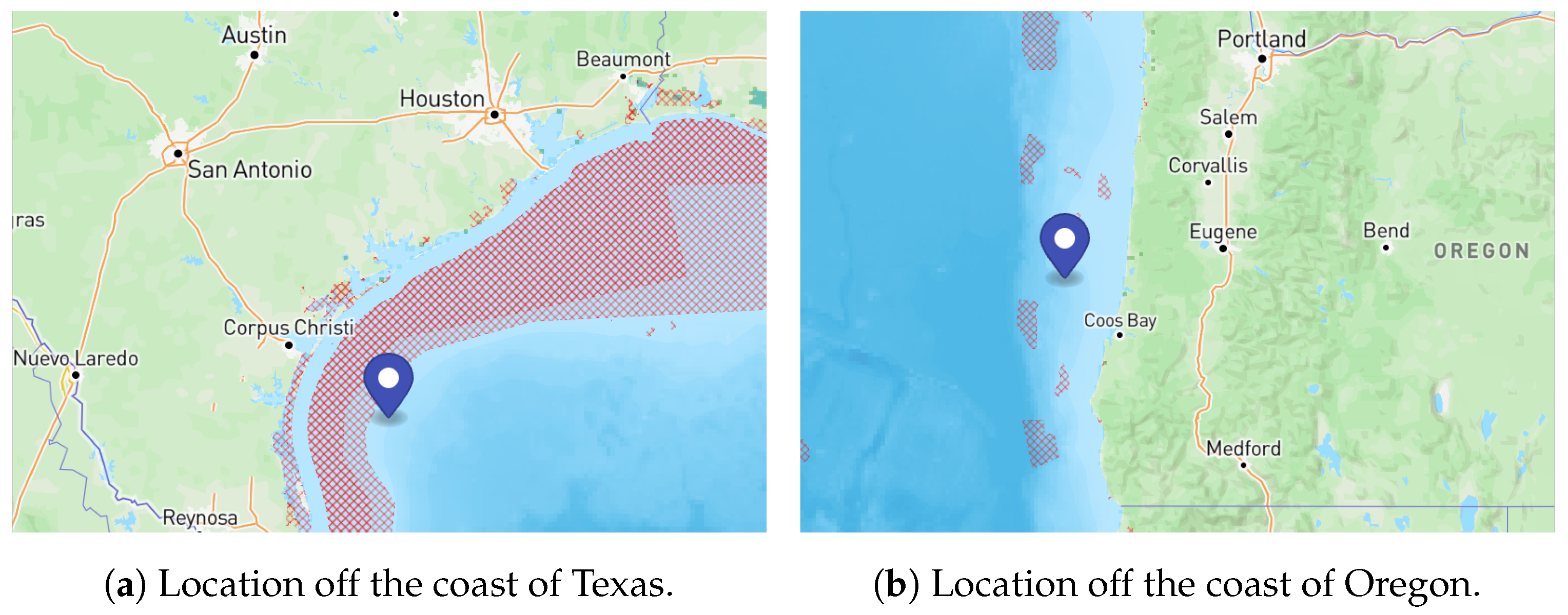
| Parameter | Texas | Oregon |
|---|---|---|
| Temperature (°C) | 25 | 12 |
| Salinity (ppt) | 36.5 | 33 |
| Depth (m) | 45 | 482 |
| Average Wind Speed (m/s) | 8.06 | 9.74 |
| Average Omnidirectional Wave Power (kW/m) | N/A | 43.75 |
| Parameter | Texas | Oregon |
|---|---|---|
| Wind Capacity (MW) | 345 | 330 |
| Wave Capacity (MW) | N/A | 30.9 |
| Battery Capacity (MW) | 50 | 50 |
| Battery Duration (MWh) | 200 | 200 |
| DOC Capacity (MW) | 356.7 | 362.1 |
| Result | Error |
|---|---|
| Maximum Total Power | <1% |
| Maximum DOC Rate | <1% |
| Maximum Total Liquid Pump Power | 2% |
| Maximum Gas Vacuum Power | 5% |
| Maximum Post-Processing Power (Purification and Compression) | 3% |
| System Result | Value |
|---|---|
| Yearly Capture | 720.4 kt/yr |
| DOC Capacity Factor | 49.5% |
| Energy Capacity Factor | 41% |
| Fraction of Time DOC is Performed | 90% |
| Maximum Tank Volume | 12,960 m3 |
| Total Plant Power Range | 6.5–357 MW |
| DOC Rate Range | 16.6–166 t/hr |
| Intake Pump (“Pump O”) Flow Rate Range | 60–600 m3/s |
| ED Power Range | 24–240 MW |
| Total Pump Power Range | 0.68–40 MW |
| Maximum Vacuum Flow Rate Range | 21.6–649.7 m3/s |
| Vacuum Power Range | 1.1–35.6 MW |
| Purification Power Range | 3.2–32.5 MW |
| Compression Power Range | 1.5–15 MW |
| Parameter | Texas | Oregon |
|---|---|---|
| Annual Renewable Energy Production (GWh) | 1087.6 | 1451.7 |
| Wind Capacity Factor (%) | 36.0 | 46.4 |
| Wave Capacity Factor (%) | N/A | 40.7 |
| Hybrid Renewable Energy System Capacity Factor (%) | 38.2 | 45.8 |
| LCOE ($/MWh) | 148 | 209 |
| DOC Capacity Factor (%) | 34.2 | 44.4 |
| Yearly Capture (kt/yr) | 495.8 | 685.6 |
| Parameter | Texas | Oregon |
|---|---|---|
| Scenario 1 (%) | 59.3 | 70.4 |
| Scenario 2 (%) | 13.8 | 11 |
| Scenario 3 (%) | 7.8 | 8.3 |
| Scenario 4 (%) | 0.7 | 1.1 |
| Scenario 5 (%) | 18.4 | 9.2 |
Disclaimer/Publisher’s Note: The statements, opinions and data contained in all publications are solely those of the individual author(s) and contributor(s) and not of MDPI and/or the editor(s). MDPI and/or the editor(s) disclaim responsibility for any injury to people or property resulting from any ideas, methods, instructions or products referred to in the content. |
© 2025 by the authors. Licensee MDPI, Basel, Switzerland. This article is an open access article distributed under the terms and conditions of the Creative Commons Attribution (CC BY) license (https://creativecommons.org/licenses/by/4.0/).
Share and Cite
Niffenegger, J.S.; Brunik, K.; Deutsch, T.; Lawson, M.; Thresher, R. Hybrid Energy-Powered Electrochemical Direct Ocean Capture Model. Clean Technol. 2025, 7, 52. https://doi.org/10.3390/cleantechnol7030052
Niffenegger JS, Brunik K, Deutsch T, Lawson M, Thresher R. Hybrid Energy-Powered Electrochemical Direct Ocean Capture Model. Clean Technologies. 2025; 7(3):52. https://doi.org/10.3390/cleantechnol7030052
Chicago/Turabian StyleNiffenegger, James Salvador, Kaitlin Brunik, Todd Deutsch, Michael Lawson, and Robert Thresher. 2025. "Hybrid Energy-Powered Electrochemical Direct Ocean Capture Model" Clean Technologies 7, no. 3: 52. https://doi.org/10.3390/cleantechnol7030052
APA StyleNiffenegger, J. S., Brunik, K., Deutsch, T., Lawson, M., & Thresher, R. (2025). Hybrid Energy-Powered Electrochemical Direct Ocean Capture Model. Clean Technologies, 7(3), 52. https://doi.org/10.3390/cleantechnol7030052