Model-Based Predictive Control of a Solar Hybrid Thermochemical Reactor for High-Temperature Steam Gasification of Biomass

Abstract

The present paper deals with both the modeling and the dynamic control of a solar hybrid thermochemical reactor designed to produce syngas through the high-temperature steam gasification of biomass. First, a model of the reactor based on the thermodynamic equilibrium is presented. The Cantera toolbox is used. Then, a model-based predictive controller (MPC) is proposed with the aim of maintaining the reactor’s temperature at its nominal value, thus preserving the reactor’s stability. This is completed by adjusting the mirrors’ defocusing factor or burning a part of the biomass to compensate for variations of direct normal irradiance (DNI) round the clock. This controller is compared to a reference controller, which is defined as a combination of a rule-based controller and an adaptive proportional–integral–derivative (PID) controller with optimized gains. The robustness of the MPC controller to forecast errors is also studied by testing different DNI forecasts: perfect forecasts, smart persistence forecasts and image-based forecasts. Because of a high optimization time, the Cantera function is replaced with a 2D interpolation function. The results show that (1) the developed MPC controller outperforms the reference controller, (2) the integration of image-based DNI forecasts produces lower root mean squared error (RMSE) values, and (3) the optimization time is significantly reduced thanks to the proposed interpolation function.

1. Introduction

The present paper explores both the modeling and dynamic control of a solar hybrid thermochemical reactor dedicated to the high-temperature steam gasification of biomass. Solar energy is concentrated with the help of tracking heliostats to heat up the solar reactor which produces hydrogen through biomass gasification. Solar gasifiers have been experimentally studied since the early 1980s, with the works of Gregg et al. [1] and Taylor et al. [2] about packed-bed and fluidized-bed technologies. Interest in solar thermochemistry has grown with climate change considerations [3], especially since the mid-2000s, leading to major innovative design investigations, as reviewed in Puig-Arnavat et al. [4]. More recent works dealing with the separation of oxidation and reduction zones for thermodynamic-cycle-based operation [5] or the separation of gasification and combustion zones for hybrid solar–autothermal operation [6] in double-loop fluidized beds are reported in the literature. A solar spouted-bed gasifier was conceived by Bellouard et al. [7], and its hybrid solar–autothermal operation was investigated successively by Boujjat et al. [8] and Curcio et al. [9]. Other experimental works have demonstrated the feasibility of such hybrid operation [10,11], but the question of the dynamic control of gasifiers is still open.

Due to unavoidable variations of direct normal irradiance (DNI), which is the direct irradiance received on a plane normal to the Sun [12]—DNI refers to photons that did not interact with the atmosphere on their way to the observer—the design of concentrated solar systems had to come with the development of control strategies. A great variety of control algorithms have been investigated in the years 1980 to 2000, essentially for the thermal regulation of solar collectors. This application implies controlling the mass flow rate of the heat transfer fluid in order to regulate the fluid’s temperature at the collector’s outlet. For instance, back in 1981, Maffezzoni and Parigi [13] have shown the advantage of dynamics compensator-based systems over proportional–integral–derivative (PID) controllers for the operation of a solar steam generator. Later advances are those of Camacho et al. [14], who monitored an oil-heating distributed collector through a self-tuning PID controller, and those of Rubio et al. [15], who implemented a fuzzy controller in the same plant. Non-linear control has then been explored in the late 1990s on the basis of simplified non-linear physical models [16] or black-box models [17]. Reviews of those early developments are found in [18,19], pointing out the importance of non-linear, high-order, model-based control methods over linearized PI- or PID-based methods when applicable.

Scientific research in the field of solar thermochemical processes, which brings an additional complexity through complex chemical mechanisms, is still rather immature. Multiple outcomes can be of interest, such as the reactor’s temperature, efficiency of the energy conversion, and the syngas production rates and yields. Thanks to a feedforward–feedback controller and a model linearized around a nominal operating point, optimized energy efficiency and product quality through the day are achieved by Petrasch et al. [20]. The implementation of a model-based predictive controller (MPC) to manage a solar–thermal reactor was investigated by Saade et al. [21], with the goal of maintaining constant the CO/CO${}_2$ ratio. As an interesting result, the proposed controller is more efficient in rejecting DNI disturbances than a multi-loop approach. In addition, an attempt to provide image-based DNI forecasts, using sky images, is recorded in this work. However, the proposed forecasting model is not able to outperform the persistence model. That same year, Muroyama et al. [22] proposed a dynamic regulation of the reactor’s temperature through the injection of oxygen and additional feedstock, aiming at triggering in situ combustion under low DNI. A PI-based system was implemented, using a linearized model of the gasifier. This kind of dynamic control was also considered in Boujjat et al. [23], with the dynamic modeling of an extrapolated spouted-bed gasifier continuously kept at 1200 ${}^{\circ }$C through day and night operation.

The PROMES-CNRS laboratory possesses a solar reactor prototype in Odeillo (France), which is designed with the help of CEA-LITEN (Figure 1). In the framework of the Horizon 2020 project SFERA (Solar Facilities for the European Research Area) III, the dynamic control of the upscaled reactor is approached. An MPC controller is developed with the aim of maintaining the reactor’s temperature at its nominal value, thus ensuring its stability. This is completed by adjusting the mirrors’ defocusing factor or by burning a part of the biomass to compensate for DNI variations round the clock. The MPC controller is compared to a reference controller, which is defined as a combination of a rule-based controller and an adaptive PID controller with optimized gains.

2. Horizon 2020 Project SFERA III

The duration of SFERA III, which is funded under the Research Infrastructure Program, is five years, starting from January 2019 and ending by December 2023. SFERA III is a collaboration of 15 partners from nine EU countries aiming at reinforcing the sustainability of the European advanced CSP (concentrating solar power) research infrastructure activities. It addresses scientific challenges and integrated research activities in the field of CSP to provide the research and development community with a new level of high-quality services. The tasks are grouped into 13 work packages (WPs) categorized into three main activities:

• networking activities to improve the cooperation between the research infrastructures, the scientific community, industries and other stakeholders;
• transnational access activities aiming at providing access to all European researchers from both academia and industry to singular scientific and technological solar research infrastructures;
• joint research activities to improve the infrastructure’s integrated services.

The work presented in this paper, which contributes to the WP 10 of the project, aims at conciliating the hybrid solar–autothermal control strategy of a gasifier with the efficient implementation of an MPC-based approach. Several strategies can be planned, such as maximizing syngas production or optimizing operating conditions for enhanced reactor stability. However, in this work and based on the developed reactor model (see Section 3), the goal is to assess optimal conditions for the chemical reactions taking place in the reactor, thus ensuring its stability. The proposed MPC controller acts on the oxygen flow rate and the mirrors’ defocusing factor in order to maintain the reactor’s temperature at its nominal value, despite a varying DNI. The control action aims at minimizing oxygen consumption while taking advantage of concentrated solar energy as much as possible. The developed reactor model is inspired by the work of Boujjat et al. [23], who computed the production of a solar biomass gasifier over one year to assess its allothermal-autothermal hybridization. In addition, for the first time, DNI forecasts—perfect forecasts, smart persistence forecasts or image-based forecasts [24]—are part of the control framework, in order to achieve better smoothing of the disturbances through the day, thus taking full advantage of a predictive approach.

3. Modeling of the Solar Reactor

3.1. Description of the Model

The gasifier is designed to be heated by both concentrated solar energy (allothermal heating) and in situ combustion (autothermal heating) [7,8], enabling a continuous conversion of biomass round the clock. For a biomass flow rate maintained constant at $1.465$ $\mathrm{t}$${\mathrm{h}}^{-1}$, the reactor parameters are set so that the nominal temperature of 1473 K is reached for a DNI value equal to 800 $\mathrm{W}$${\mathrm{m}}^{-2}$, which corresponds to around 80% of the maximum DNI obtained during a year. Two chemical mechanisms can therefore occur simultaneously.

• When no oxygen is injected—DNI is higher than 800 Wm${}^{-2}$—only the endothermic gasification of biomass occurs, with an enthalpy change $\Delta H_r^o=143$kJ mol${}^{-1}$. This reaction is as follows:

  $$\begin{array}{c}\hfill {\mathrm{CH}}_{1.66}{\mathrm{O}}_{0.69}+0.31{\mathrm{H}}_2\mathrm{O}\to \mathrm{CO}+1.14{\mathrm{H}}_2\end{array}$$

  (1)
• When oxygen is injected—DNI is lower than 800 $\mathrm{W}{\mathrm{m}}^{-2}$—combustion occurs in the cavity along with gasification, with an enthalpy change $\Delta H_r^o=-452$ kJ mol${}^{-1}$. Combustion of the biomass resource—the reaction is exothermic—can be described as follows:

  $$\begin{array}{c}\hfill {\mathrm{CH}}_{1.66}{\mathrm{O}}_{0.69}+1.07{\mathrm{O}}_2\to {\mathrm{CO}}_2+0.83{\mathrm{H}}_2\end{array}$$

  (2)

These reactions actually involve numerous, complex sub-mechanisms [8]. In this work, thermodynamic equilibrium calculations are therefore employed to deduce the reactor’s chemical outcome and the related global reaction enthalpy ($Q_{reaction}$). The open-source software Cantera [25] version 2.5.1 is used in this work. These calculations are coupled with unsteady thermal balances on the reactor walls ($Q_{Sun}$, $Q_{radloss}$ and $Q_{conloss}$):

$$\begin{array}{ll}\{& \begin{array}{l}{Q}_{reaction}=\sum _{i=1}^{n_r}{f}_i^{in}{h}_i\left(T_{amb}\right)-\sum _{i=1}^{n_p}{f}_i^{out}{h}_i\left(T\right)\hfill \\ Q_{Sun}=D·C·{\eta }_{opt}·A_{aperture}·\mathrm{DNI}\hfill \\ Q_{radloss}=\sigma ·A_{aperture}·(T^4-T_{amb}^4)\hfill \\ Q_{conloss}=(T-T_{amb}) R\hfill \end{array}\end{array}$$

(3)

where $h_i$ is the enthalpy of reactants and products, $f_i^{in}$ and $f_i^{out}$ are the flow rates of reactants and products, respectively, $n_r$ and $n_p$ are the number of reactants and products, respectively, D is the defocusing factor—D ranges from 0 (all solar flux is cut) to 1 (no defocusing of the solar field), $Q_{reaction}$ is the power gained from the chemical reaction—$Q_{reaction}$ is negative (respectively positive) when the reaction is globally endothermal (respectively exothermal), $Q_{Sun}$ is the power gained from the Sun, $Q_{radloss}$ is the power lost by radiation, $Q_{conloss}$ is the power lost by conduction, m is the mass of the reactor walls, $C_{p,w}$ is the specific heat of the reactor walls, C is the concentration factor, ${\eta }_{opt}$ is the optical efficiency, $A_{aperture}$ is the aperture’s area, $\sigma$ is the Stefan–Boltzmann constant, $T_{amb}$ is the ambient temperature, and R is the globalized conduction thermal resistance.

The solar power input is proportional to DNI: it depends on the defocusing factor D, the concentration factor C, the optical efficiency ${\eta }_{opt}$, and the cavity aperture area $A_{aperture}$. This aperture is minimized so that the radiation losses are as low as possible. A global conduction loss is modeled as well to account for heat transfer through the insulation. Finally, the $Q_{reaction}$ term represents the power required to convert the cold reactants into a syngas at the reactor’s temperature. It is computed via a heterogeneous thermodynamic equilibrium between a pure solid carbon phase and a gaseous phase [26]. The solid phase is modeled as graphite carbon, and it is supposed to be fully consumed at over-stoichiometric H₂O injection rates. However, it should be mentioned that incomplete conversion may still occur at temperatures lower than 800 ${}^{\circ }$C, whatever the quantity of injected steam [27]. The gas phase is modeled as a mixture of H₂, CO, CO₂, CH₄, H₂O, O₂ and Ar, whose properties are given by the NASA GRI-MECH 3.0 database [28]. The elemental chemical composition of the mixture is determined by the wood input flow rate, its moisture fraction (8.9% in weight), and its molecular composition (CH_1.66O_0.69, on a dry basis). The high heating value (HHV) of the reference wood sample, measured by calorimetry, is also provided to compute the corresponding standard enthalpy of formation, enabling the calculation of the inlet flow enthalpy. The outlet flow enthalpy at the reactor’s temperature is directly given by the Cantera function. All these heat transfers are applied to the reactor wall and determine the impact of both DNI variations and chemical inputs on the reactor’s temperature. Thus, the reactor’s temperature can be modeled through the following first-order non-linear ordinary differential which represents the heat balance of the reactor:

$$\begin{array}{ll}\{& \begin{array}{l}m·C_{p,w}·\frac{\mathrm{d}T}{\mathrm{d}t}=Q_{re}(f_{steam}^{in},f_{biomass}^{in},f_{oxygen}^{in},T)+Q_{net}\hfill \\ Q_{net}=Q_{Sun}-Q_{radloss}-Q_{conloss}\hfill \end{array}\end{array}$$

(4)

where $Q_{net}$ results from the power gained from the Sun and the power lost due to radiation and conduction.

Note that above a DNI value of 800 $\mathrm{W}{\mathrm{m}}^{-2}$, a reduction of the input solar power is necessary to maintain the reactor’s temperature at 1473 K. As a result, D is introduced. Below this DNI value, oxygen is added to heat the reactor thanks to in situ combustion, which directly alters the syngas composition by shifting the thermodynamic equilibrium. Finally, when DNI is lower than 150 $\mathrm{W}{\mathrm{m}}^{-2}$, the reactor’s aperture is closed to limit the radiation loss.

3.2. Simulation of the Model

As shown in the previous section, the reactor’s temperature T is modeled by a non-linear ordinary differential equation. DNI and the reactants’ flow rates (biomass, oxygen, and steam) are the model inputs. In this section of the paper, the model is simulated by solving this differential equation according to different scenarios, with varying DNI profiles and reactants’ flow rates.

3.2.1. Without Oxygen Injection

First, with a constant biomass flow rate $f_{biomass}^{in}$ of $1.465$ $\mathrm{t}{\mathrm{h}}^{-1}$ and starting from an initial reactor’s temperature T of 1073 K, the model’s response to three DNI steps of different amplitudes is simulated (from 0 to 700 Wm${}^{-2}$, 800 Wm${}^{-2}$ and 900 Wm${}^{-2}$, respectively). As can be seen in Figure 2, when DNI = 800 Wm${}^{-2}$, the steady-state temperature is equal to 1473 K, which is the reactor’s nominal temperature. For DNI = 700 Wm${}^{-2}$, this nominal temperature is not reached: oxygen should be injected to compensate for the lack of power. On the contrary, when DNI = 900 Wm${}^{-2}$, the temperature exceeds this nominal temperature: in this case, the concentration mirrors should be defocused to decrease the reactor’s temperature. The static gain, the time constant $\tau$ (i.e., the time needed to reach 63% of the steady-state value), and the rise time $T_r$ (i.e., the time needed to rise from 10 to 90% of the total variation) all depend on the amplitude of the DNI step. The estimated value of these three parameters can be found in

Table 1. First-order dynamic model corresponding to the temperature curves shown in Figure 2.

DNI [Wm${}^{-2}$]	Static Gain [-]	$\mathit{\tau }$ [min]	${\mathit{T}}_{\mathit{r}}$ [min]
700	0.3	31.5	69.3
800	0.5	26.3	58
900	0.6	23	50.6

: with higher DNI values, the static gain increases, while $\tau$ and $T_r$ decrease, rendering the system faster. This means that not only does the solar reactor reach higher temperatures with higher DNI values, but it also does so faster. This change in the system dynamics must be taken into consideration for an accurate reactor’s temperature control.

The power balance corresponding to the steady state of the three considered DNI steps is given in Figure 3. When DNI increases, the conduction loss remains approximatively the same, while the radiation loss increases and the power of the chemical reaction decreases. The effect of sudden DNI variations on the reactor’s temperature—with nominal design values, i.e., T = 1473 K, DNI = 800 Wm${}^{-2}$, and $f_{biomass}^{in}$ = 1.465 th${}^{-1}$—is shown in Figure 4. The first variation—a DNI drop of 200 Wm${}^{-2}$—causes the reactor’s temperature to drop by 13.13 K; the reactor’s nominal temperature is reached again after approximatively 90 min. The second variation—a DNI rise of 200 Wm${}^{-2}$—increases the reactor’s temperature by 13.43 K. This simulation shows that sudden DNI variations have a strong effect on the reactor’s temperature, which could be compensated depending on the reactor’s input, if accurate DNI forecasts are provided to the controller. In addition, the long duration before the reactor’s temperature reaches its nominal value after the DNI pulses can be minimized by injecting oxygen, which can help increase the reactor’s temperature faster, as will be shown in Section 3.2.2.

Finally, the evolution of the reactor’s temperature against different biomass flow rates is shown in Figure 5. Here, DNI is set to 900 $\mathrm{W}$${\mathrm{m}}^{-2}$. It can be observed that as the biomass flow rate increases, the temperature decreases and more syngas is produced. However, it should be mentioned that the biomass flow rate cannot be a control input, since the model used in this work does not take the inertia of the gasification reaction into consideration.

3.2.2. With Oxygen Injection

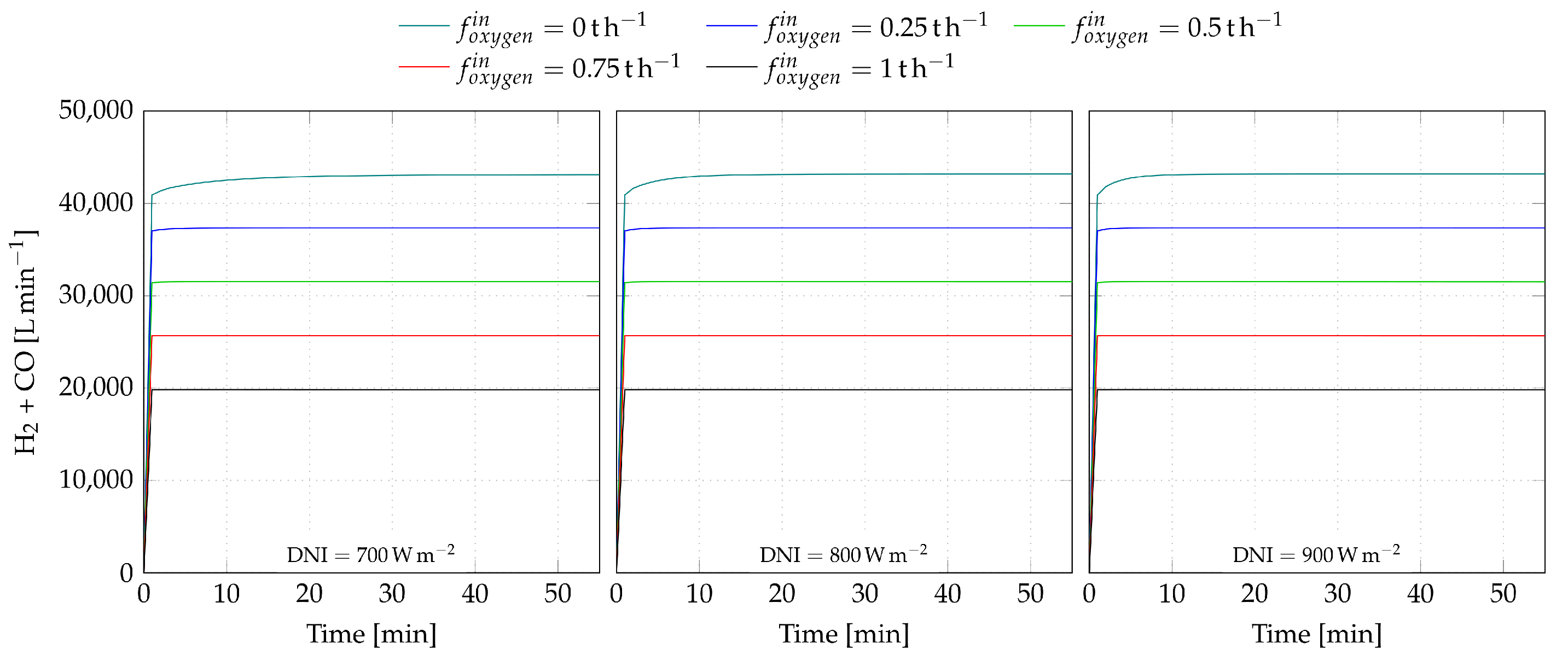
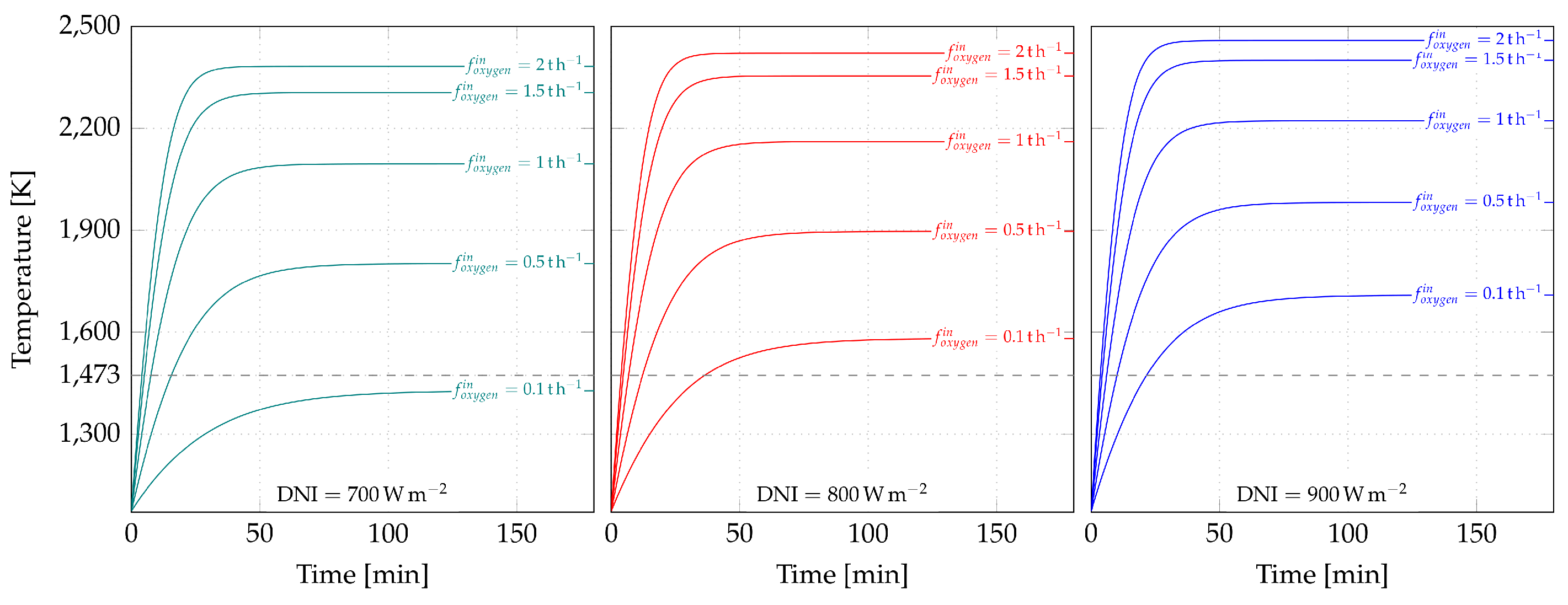
The reactor’s temperature can be decreased by either increasing the biomass flow rate or by varying the energy received from the Sun, using the defocusing factor D. However, in case of DNI deficit (less than 800 $\mathrm{W}$$\mathrm{m}$${}^{-2}$), to increase the temperature without decreasing the biomass flow rate, oxygen has to be injected to burn the biomass. Since the burnt biomass is not used in the gasification process, less syngas is produced, as shown in Figure 6. In addition, the results of the simulation presented in Figure 7 show that oxygen injection can increase the reactor’s temperature rapidly. For $\mathrm{DNI}=800 \mathrm{W}{\mathrm{m}}^{-2}$, the reactor crossed the 1473 K level after only 4 min with $f_{oxygen}^{in}=2 \mathrm{t}{\mathrm{h}}^{-1}$. As shown in Figure 4, this input can correct the reactor’s temperature rapidly in case of sudden DNI deficit. As shown in Figure 8, when $\mathrm{DNI}<150 \mathrm{W}{\mathrm{m}}^{-2}$, the reactor’s aperture is closed, and its temperature can be maintained by injecting $0.88$ $\mathrm{t}$${\mathrm{h}}^{-1}$ of oxygen.

4. Control of the Solar Reactor

In this section, the reference controller, the MPC controller and the DNI forecast model are presented. The following discretized reactor model $\mathcal{M}$ is used:

$$\begin{array}{c}\hfill T(k+1)=\mathcal{M}(D\left(k\right),f_{oxygen}^{in}\left(k\right),T\left(k\right))\end{array}$$

(5)

with $t=k·T_s$ ($T_s=30\mathrm{s}$ is the sampling time). The biomass flow rate $f_{biomass}^{in}$ and the steam flow rate $f_{steam}^{in}$ are fixed to their nominal design values of $1.465$ $\mathrm{t}$${\mathrm{h}}^{-1}$ and $0.26$ $\mathrm{t}$${\mathrm{h}}^{-1}$, respectively. The goal is to maintain the reactor’s temperature at $(1473 \pm 15) \mathrm{K}$ in order to ensure its stability. The control variables are the oxygen flow rate $f_{oxygen}^{in}$ and the defocusing factor D. In case of a DNI deficit ($\mathrm{DNI}⩽800 \mathrm{W} {\mathrm{m}}^{-2}$), oxygen can be injected to increase the reactor’s temperature by burning biomass. In case of an excess of DNI ($\mathrm{DNI}>800 \mathrm{W} {\mathrm{m}}^{-2}$), the solar field can be defocused to compensate for this excess.

4.1. Reference (PID/RB) Controller

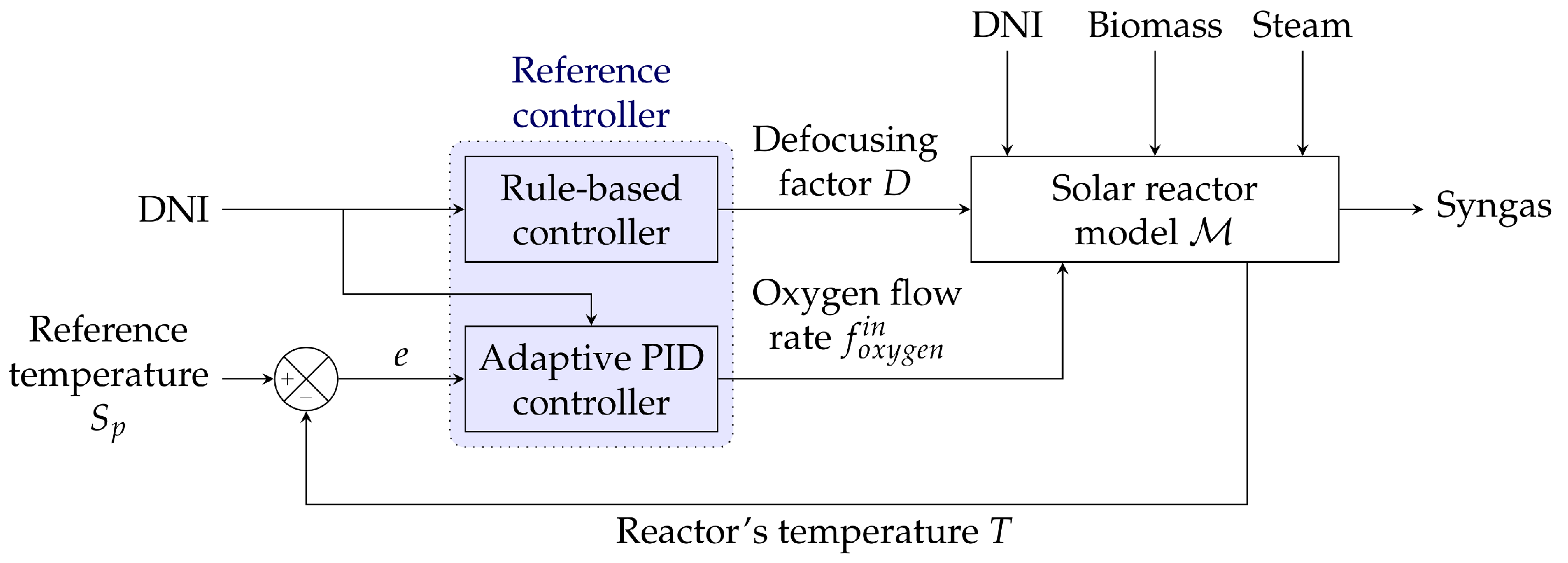
The reference controller is a combination of an adaptive PID controller with optimized gains (Section 4.1.1) and a rule-based controller (Section 4.1.2) (Figure 9).

4.1.1. Adaptive PID Controller for the Oxygen Flow Rate

The oxygen flow rate $f_{oxygen}^{in}$ is managed by an adaptive PID controller with optimized gains. An optimized adaptive PID controller is implemented to perform a closed loop control of the oxygen injection. It can be described as follows:

$$\begin{array}{c}\hfill f_{oxygen}^{in}\left(k\right)=K_p·e\left(k\right)+K_i·\sum _{i=1}^{k}e\left(i\right)+K_d·\frac{e\left(k\right)-e(k-1)}{T_s}\mathrm{with}e\left(k\right)=S_p-T\left(k\right)\end{array}$$

(6)

where $S_p$ is the temperature setpoint, and T is the reactor’s temperature, and [29]:

• $K_p$ is the proportional gain, helping the controller reach the setpoint faster, with the risk of overshooting; a small value will result in an important steady-state error;
• $K_i$ is the integral gain, helping to eliminate the steady-state error; a large value can result in a longer settling time and higher oscillations;
• $K_d$ is the derivative gain, generating a fast response and a stabilizing effect in dynamic regime.

An adaptive PID controller, where gains change with the measured DNI, is implemented. This choice is motivated by the fact that the reactor’s functioning depends on the DNI. Three intervals of DNI values are considered.

• $\mathrm{DNI}<150 \mathrm{W} {\mathrm{m}}^{-2}$: The reactor’s aperture is closed ($A_{aperture}=0$) to limit radiative losses, which affects the thermal equilibrium of the system. The PID controller manages the system by injecting a minimum of 0.88 th${}^{-1}$ of oxygen.
• $150 \mathrm{W} {\mathrm{m}}^{-2}⩽\mathrm{DNI}⩽800 \mathrm{W} {\mathrm{m}}^{-2}$: The reactor’s aperture is open, and the amount of DNI received is not sufficient to maintain the reactor’s temperature without oxygen injection. The PID controller determines the oxygen flow rate allowing to minimize the error between the setpoint and the measured temperature.
• $\mathrm{DNI}>800 \mathrm{W} {\mathrm{m}}^{-2}$: The excess of DNI forces the PID controller to recommend a minimal oxygen flow rate allowing the reactor to cool down and play on defocusing if the reactor’s temperature is higher than the setpoint.

For each interval of DNI values, the optimized PID gains are obtained as follows:

$$\begin{array}{c}\hfill (K_p,K_i,K_d)=argmin\sum _{k=1}^n{(S_p-T\left(k\right))}^2\end{array}$$

(7)

where $K_p$, $K_i$ and $K_d$ are the PID gains, $S_p$ is the temperature setpoint, T is the reactor’s temperature, and n is the number of time steps.

This tuning strategy, targeting a certain performance described by Equation (7), is considered to be the optimal approach to design a PID controller [30]. The optimized PID gains are given in

Table 2. Optimized gains of the adaptive PID controller.

	DNI < 150 Wm${}^{-2}$	150 Wm${}^{-2}$ ⩽ DNI ⩽ 800 Wm${}^{-2}$	DNI > 800 Wm${}^{-2}$
$K_p$	1.6 × 10${}^{-2}$	3.4 × 10${}^{-2}$	1.5 × 10${}^{-3}$
$K_i$	0	9.0 × 10${}^{-4}$	1.5 × 10${}^{-4}$
$K_d$	1.2 × 10${}^{-2}$	2.5 × 10${}^{-2}$	1.0 × 10${}^{-5}$

. Note that the gains are significantly lower when $\mathrm{DNI}>800 \mathrm{W} {\mathrm{m}}^{-2}$, which is explained by the necessity to inject less oxygen in this case, to allow the reactor to cool down. In addition, in all cases, $K_i$ is significantly lower than the other gains except when $\mathrm{DNI}>800 \mathrm{W} {\mathrm{m}}^{-2}$, where the PID gains should be low to inject oxygen with a minimal flow rate, which permits the solar reactor to cool down if needed. This means that the optimizer found that the optimal performance, based on the provided objective function, does not need the integral effect.

4.1.2. Rule-Based Controller for the Defocusing Factor

The defocusing factor D is governed by a rule-based (RB) controller, which is defined as follows:

• if $\mathrm{DNI}\left(k\right)>800 \mathrm{W} {\mathrm{m}}^{-2}$ and $T\left(k\right)>1473$ K, $D\left(k\right)=800 \mathrm{DNI}\left(k\right)$;
• if $\mathrm{DNI}\left(k\right)⩽$ 800 Wm${}^{-2}$ and $T\left(k\right)<1473$ K, $D\left(k\right)=1$.

In the first case, solar energy utilization is maximized, while in the second case, there is an excess of DNI and, provided the solar reactor is at its nominal temperature, defocusing is used to supply a power equivalent to the one obtained when DNI = 800 Wm${}^{-2}$.

4.2. MPC Controller

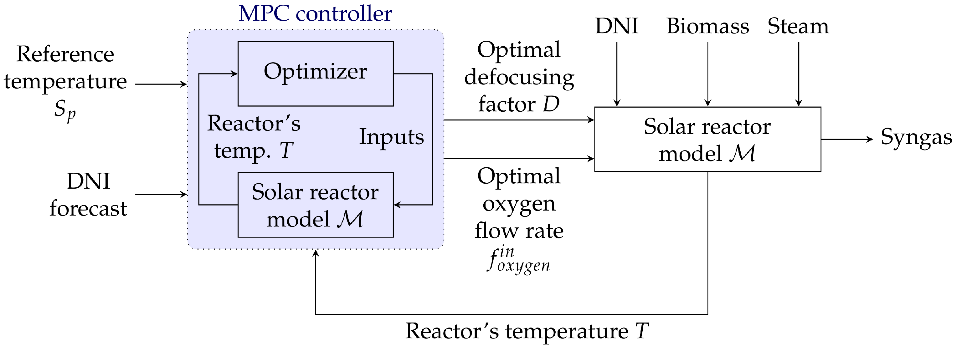
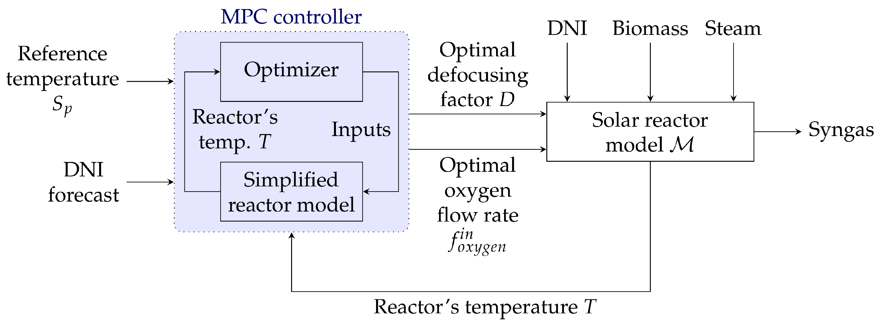
The proposed MPC controller can find the optimal sequence of inputs based on both the model of the reactor (see Section 3) and the provided DNI forecasts (see Section 4.3). Of course, this is a huge advantage for the problem at hand, since the solar reactor is very sensitive to DNI variations (the MPC controller aims at compensating for such variations). In addition, based on the required performance and constraints, the MPC controller can find the optimal combination of multiple inputs simultaneously. The objective is still to maintain the reactor’s temperature at 1473 K, thus preserving the reactor’s stability, while taking advantage of the available solar energy and minimizing oxygen consumption. The controller’s structure is depicted by Figure 10. Let n be the number of time steps in the prediction horizon of the controller (which is less than 2.5 min). At each of those n time steps, the optimization problem formulated below is solved to find the optimal inputs $\mathit{D}\in {\mathbb{R}}^n$ and ${\mathit{f}}_{oxygen}^{in}\in {\mathbb{R}}^n$ [31]:

$$\begin{array}{c}\hfill (D{}^{★},f_{oxygen}^{in★})=argmin\sum _{i=1}^n\alpha {\left(S_p-T(k+i)\right)}^2+\beta {\left(f_{oxygen}^{in}(k+i)\right)}^2-\gamma {\left(D(k+i)\right)}^2\end{array}$$

(8)

where $T(k+1)=\mathcal{M}(D\left(k\right),f_{oxygen}^{in}\left(k\right),T\left(k\right))$, $0⩽D(k+i)⩽1$ and $0⩽f_{oxygen}^{in}(k+i)⩽2$.

The goal here is to make a trade-off between following the temperature setpoint, minimizing oxygen consumption, and maximizing the use of solar energy. This trade-off is determined by the weights $\alpha$, $\beta$, and $\gamma$. These weights are chosen so that the minimization of the oxygen consumption (determined by $\beta$) and the maximization of the exploited solar energy (determined by $\gamma$) do not degrade the temperature tracking performance severely. Here, $\alpha =5$, $\beta =5$ and $\gamma =10$. The higher weight on the defocusing factor D ensures that the reactor receives the highest possible solar energy while using as little oxygen as possible. This performance comes at the cost of a higher temperature-tracking error. DNI forecasts are needed to solve the optimization problem (see Section 4.3). The optimizer used is the trust-region constrained algorithm, which is able to solve non-linear optimization problems and is highly robust [32].

4.3. DNI Forecasting

Several forecasting approaches can be considered, depending on the required forecast horizon. Statistical models, which are trained on a dataset of past DNI observations to learn patterns, can be considered [33,34,35,36], as well as image-based models, where sky images are processed to extract information related to the sky situation that will affect DNI [37,38,39,40,41]. In this work, DNI forecasts must be provided to the MPC controller for every time step in its prediction horizon, which is very short (less than 2.5 min). For such short forecast horizons, persistence models score very low forecast errors. However, they fail to predict DNI ramps, which are very influential, as shown in Figure 4. Thus, a model scoring low forecast errors and capable of forecasting most DNI ramps is needed. This eliminates models based on past DNI observations only and justifies the integration of ground-based sky images with high spatial–temporal resolution. Therefore, in this work, the proposed model relies on a hybridization between statistical and image-based models. The forecast horizon $H=h·T_s$, with $T_s$ = 30 s. To evaluate the robustness of the MPC controller to forecast errors, perfect forecasts and smart persistence forecasts are also considered.

4.3.1. Database

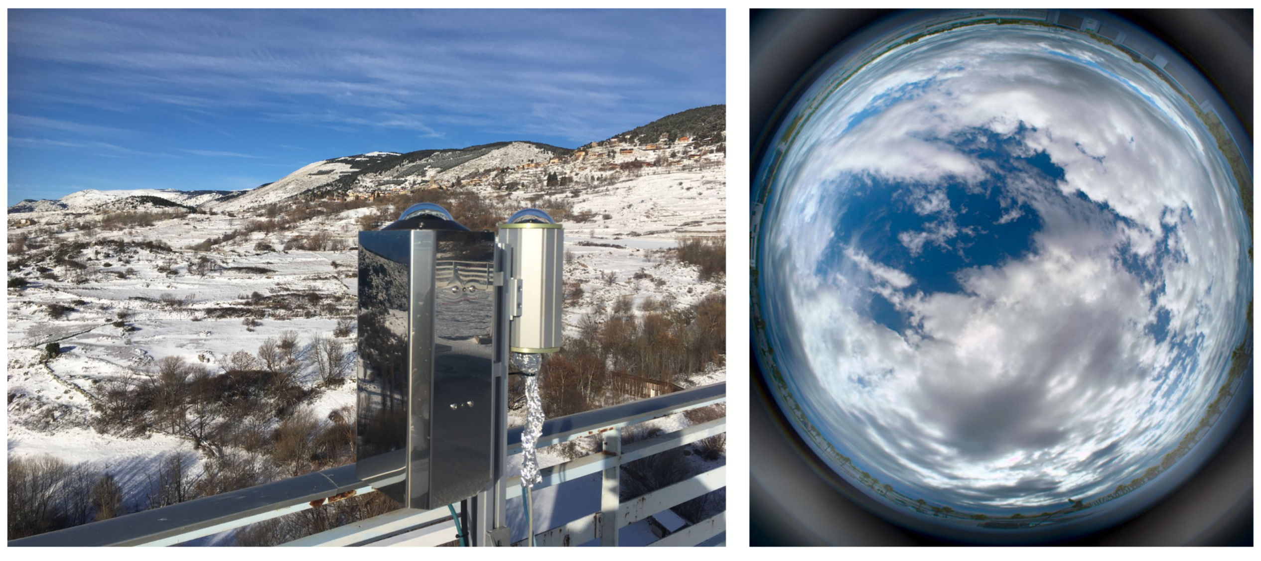
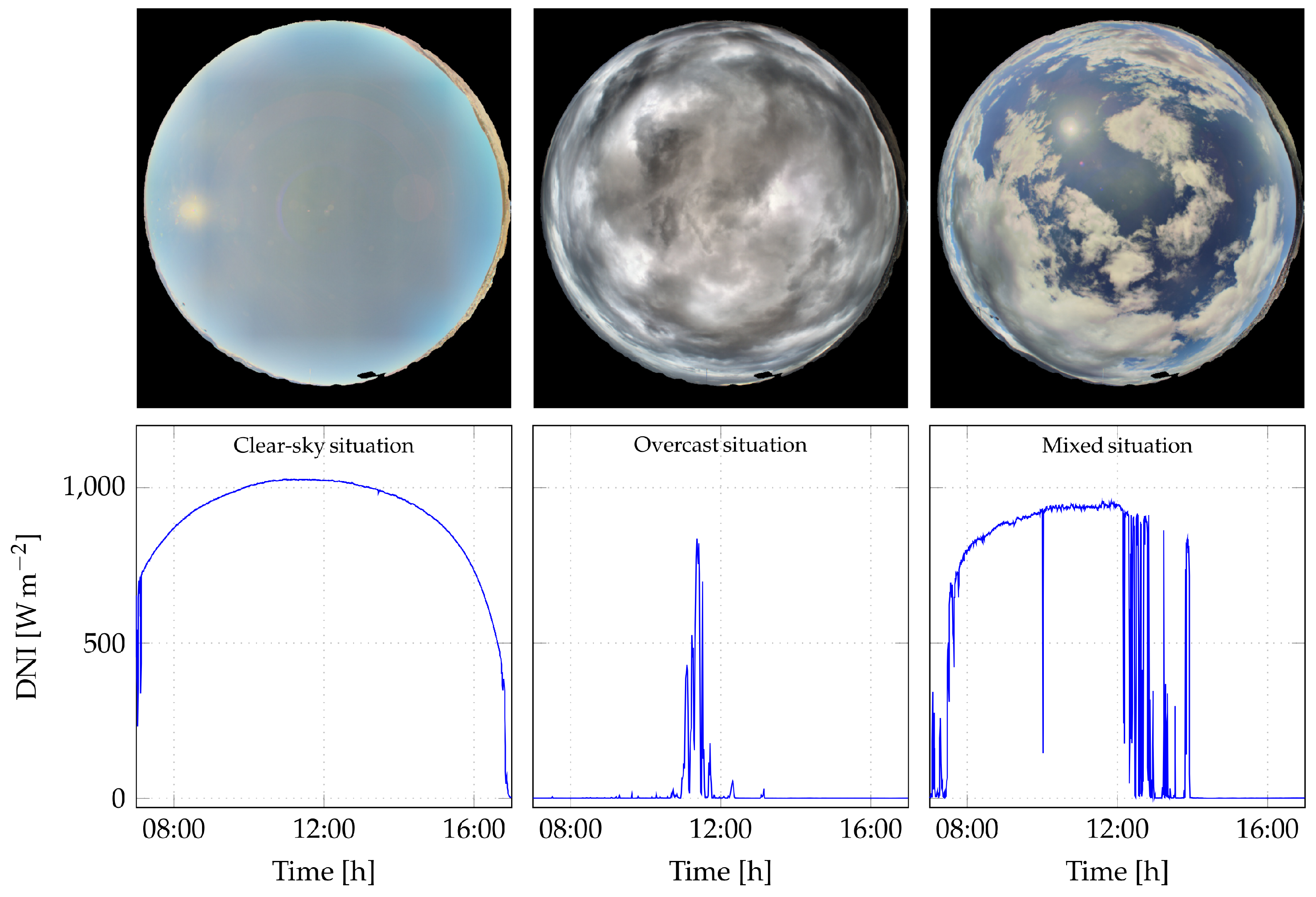
The database (Odeillo) used in this study consists of sky images, provided by the new-generation digital imaging system developed by PROMECA with the help of PROMES-CNRS (Figure 11), and DNI measurements ($T_s$ = 30 s) obtained using a pyrheliometer Kipp & Zonen CH1 and a low-voltage high-precision industrial Modbus data acquisition module Gantner A4. Sun tracking is made in open loop by a 2-axis robot Kipp & Zonen 2 GD. There are no missing data (373 days): 128 clear-sky days (34.4%), 49 overcast days (13.1%), and 196 days with mixed situations (52.5%) (Figure 12). Mixed situations are the most difficult situations to handle because of the highly variable atmospheric conditions.

The sky imager is a continuously operating digital imaging system designed to capture sky images with a fisheye lens (the field of view is 180${}^{\circ }$). Its main hardware/software features are high-end color CMOS (complementary metal oxide semiconductor) 1.5 MP sensor and high dynamic range (HDR) imaging. HDR images, obtained every 30 s, are key for the efficient detection of clouds, in particular in the circumsolar area, where pixel values are saturated in low dynamic range (LDR) images, even though it contains important information for very short-term DNI forecasting.

4.3.2. Smart Persistence Forecasts

DNI can be split into two quantities: the clear-sky DNI—${\mathrm{DNI}}_{\mathrm{CS}}$ in the sequel—and the clear-sky index $K_c$. ${\mathrm{DNI}}_{\mathrm{CS}}$ is the solar power received at the ground level per unit of area, at a specific location, when there is no cloud between the Sun and the observer. The clear-sky index is derived from the attenuation of DNI caused by sun-blocking clouds. So:

$$\begin{array}{c}\hfill \mathrm{DNI}\left(k\right)=K_c\left(k\right)·{\mathrm{DNI}}_{\mathrm{CS}}\left(k\right)⟺K_c\left(k\right)=\frac{\mathrm{DNI}\left(k\right)}{{\mathrm{DNI}}_{\mathrm{CS}}\left(k\right)}\end{array}$$

(9)

The smart persistence model assumes that the clear-sky index $K_c$ remains constant over the forecast horizon, i.e., between time k and time $k+h$:

$$\begin{array}{c}\hfill \widehat{\mathrm{DNI}}(k+h)=K_c\left(k\right)·{\widehat{\mathrm{DNI}}}_{\mathrm{CS}}(k+h)=\frac{\mathrm{DNI}\left(k\right)}{{\mathrm{DNI}}_{\mathrm{CS}}\left(k\right)}·{\widehat{\mathrm{DNI}}}_{\mathrm{CS}}(k+h)\end{array}$$

(10)

The smart persistence model thus needs clear-sky DNI forecasts. In this work, the model developed by Ineichen and Perez [42] is used with $T_{LI}$ forecast using the method proposed by Nou et al. [43]:

$$\begin{array}{c}\hfill {\widehat{\mathrm{DNI}}}_{\mathrm{CS}}(k+h)=b·I_0(k+h)·e^{-0.09m(k+h)·(T_{LI}\left(k\right)-1)}\end{array}$$

(11)

where b is a function of the altitude of the considered site, $I_0$ is the extraterrestrial solar irradiance, m is the relative optical air mass and $T_{LI}$ is the Linke turbidity coefficient.

4.3.3. Image-Based Forecasts

The proposed image-based model, inspired by the forecast model developed by Karout et al. [24], is a hybridization between the persistence model and an LSTM model. Its global architecture is shown in Figure 13. It processes HDR images and DNI measurements to forecast sudden DNI variations (DNI ramps), and it can be described as follows.

• An HDR image is processed to detect clouds using a segmentation model and estimate their motion with the aim of localizing the part of the image that will interact with the Sun at time $k+h$. This region is called the region of interest (ROI) in the sequel.
• The cloud fraction (CF) in the ROI (${\mathrm{CF}}_{{\mathrm{ROI}}_h}$) is calculated. ${\mathrm{CF}}_{{\mathrm{ROI}}_h}$ is defined as the ratio of the number of cloud pixels to the number of clear-sky pixels in the ROI.
• The model decides if a ramp will occur by analyzing the variation of ${\mathrm{CF}}_{{\mathrm{ROI}}_h}$ between two consecutive time steps. If this variation is greater than 3% of the maximum value of ${\mathrm{CF}}_{{\mathrm{ROI}}_H}$, then a ramp is expected. This value is chosen to avoid ramp detection due to noise in the ${\mathrm{CF}}_{{\mathrm{ROI}}_H}$ signal. This approach also determines the ramp’s direction, since an increase in ${\mathrm{CF}}_{{\mathrm{ROI}}_H}$ indicates a possible decrease in DNI and vice versa.
• The absolute value of the ramp magnitude RM is forecast using a long short-term memory (LSTM) network (see

  Table 3. Optimal LSTM architecture for each forecast horizon H.

  H [min]	Time Support (Observations)	LSTM Layers (Units)				Fully Connected Layers (Units)
  		1st	2nd	3rd	4th	1st	2nd	3rd
  0.5	8	179	229	204	104	20	5	5
  1	8	254	204	219	229	20	5	⌀
  1.5	8	229	54	204	179	5	20	20
  2	8	254	104	79	229	5	20	20
  2.5	8	154	179	104	4	5	5	⌀

  for the optimal LSTM architecture, according to the forecast horizon H, which is determined using an optimization framework [44]).
• The DNI forecast at time $k+h$ is obtained by a persistence (if no ramp is expected) or a persistence to which the ramp magnitude RM is added (if a ramp is expected):

  $$\begin{array}{c}\widehat{\mathrm{DNI}}(k+h)=\mathrm{DNI}\left(k\right)+\delta \left(k\right)·\widehat{\mathrm{RM}}\left(k\right)\end{array}$$

  (12)

  where $\mathrm{DNI}$ is the measured DNI, $\widehat{\mathrm{RM}}$ is the forecast ramp magnitude and $\delta$ is calculated as follows:

  $$\delta \left(k\right)=\{\begin{array}{cc}1,\hfill & \mathrm{if}\Delta {\mathrm{CF}}_{{\mathrm{ROI}}_H}\left(k\right)<-7.65\hfill \\ -1,\hfill & \mathrm{if}\Delta {\mathrm{CF}}_{{\mathrm{ROI}}_H}\left(k\right)>7.65\hfill \\ 0,\hfill & \mathrm{else}\hfill \end{array}$$

  (13)

  with $\Delta {\mathrm{CF}}_{{\mathrm{ROI}}_H}\left(k\right)={\mathrm{CF}}_{{\mathrm{ROI}}_H}\left(k\right)-{\mathrm{CF}}_{{\mathrm{ROI}}_H}(k-1)$.

4.3.4. Performance Criteria

Four performance criteria are used here to evaluate the models:

• The root mean squared error (RMSE) is calculated as follows:

  $$\begin{array}{c}\mathrm{RMSE}=\sqrt{\frac{1}{n_{obs}}\sum _{k=1}^{n_{obs}}{\left(\mathrm{DNI}\left(k\right)-\widehat{\mathrm{DNI}}\left(k\right)\right)}^2}\end{array}$$

  (14)

  where $n_{obs}$ is the number of observations, $\mathrm{DNI}$ is the measured DNI and $\widehat{\mathrm{DNI}}$ is the predicted DNI.
• The skill factor (SF) is employed to evaluate the models’ performance versus the smart persistence model (a positive skill factor means that the proposed model outperforms the smart persistence model). It is defined as follows:

  $$\mathrm{SF}=100·\left(1-\frac{{\mathrm{RMSE}}_{\mathrm{M}}}{{\mathrm{RMSE}}_{\mathrm{SPM}}}\right)$$

  (15)

  where ${\mathrm{RMSE}}_{\mathrm{M}}$ and ${\mathrm{RMSE}}_{\mathrm{SPM}}$ are the nRMSE of the evaluated model and the smart persistence model, respectively.
• The mean average error (MAE) is calculated as follows:

  $$\begin{array}{c}\mathrm{MAE}=\frac{1}{n_{obs}}\sum _{k=1}^{n_{obs}}\left(\mathrm{DNI}\left(k\right)-\widehat{\mathrm{DNI}}\left(k\right)\right)\end{array}$$

  (16)

  where $n_{obs}$ is the number of observations, $\mathrm{DNI}$ is the measured DNI and $\widehat{\mathrm{DNI}}$ is the forecast DNI.
• Finally, a criteria called ramp detection index (RDI) is used [45]. It is designed to evaluate the ability of the model to predict ramps, which have an important impact on CSP plants: predicting them can thus be helpful in the control process. First, the ramp magnitude (RM) is calculated as:

  $$\mathrm{RM}\left(k\right)=\frac{\left|\mathrm{DNI}\left(k\right)-\mathrm{DNI}(k+h)\right|}{{\widehat{\mathrm{DNI}}}_{\mathrm{CS}}\left(k\right)}$$

  (17)

  where ${\widehat{\mathrm{DNI}}}_{\mathrm{CS}}$ is the estimated clear-sky DNI.
  Usually, high-magnitude DNI ramps are defined by $\mathrm{RM}\left(k\right)>0.5$ and moderate DNI ramps are defined by $0.3<\mathrm{RM}\left(k\right)<0.5$. A ramp detection (also called a hit) is achieved if the two following conditions are satisfied:

  $$\begin{array}{cc}\hfill \mathrm{RM}\left(k\right)& >0.15\hfill \end{array}$$

  (18)

  $$\begin{array}{cc}\hfill sign(\mathrm{DNI}\left(k\right)-\widehat{\mathrm{DNI}}(k+h))& =sign\left(\mathrm{DNI}\right(k)-\mathrm{DNI}(k+h\left)\right)\hfill \end{array}$$

  (19)

  where $\widehat{\mathrm{DNI}}$ and $\mathrm{DNI}$ are the forecast and measured DNI, respectively.
  The chosen $\mathrm{RM}$ value represents ramps with high occurrence probability, thus increasing the challenge of scoring a high RDI by increasing the number of considered ramps in the RDI calculation. The ramp is not detected (a miss) if Equation (20) is met while Equation () is not. Finally, the ramp detection index is calculated as follows:

  $$\mathrm{RDI}=\frac{N_{hit}}{N_{hit}+N_{miss}}$$

  (20)

  where $N_{hit}$ and $N_{miss}$ are the numbers of hits and misses, respectively.

4.3.5. Forecasting Results

The LSTM neural networks (see Table 3) are trained and validated using 17 days of mixed situations (representing 20,400 observations) with various DNI profiles: 12 days (70% of the dataset) are used for training and 5 days (30% of the dataset) are used for validation. In addition, 7 days with clear-sky, overcast, and mixed situations (see Figure 12) are used to test the model. The loss function is the mean average error (MAE), which proved to be a better choice than other possible loss functions for this application. The image-based model performs well on the validation dataset, which means that it did not overfit. The image-based model outperforms the smart persistence model on all days in the test dataset for each forecast horizon (Figure 14). As expected, RMSE and MAE increase as the forecast horizon increases, since forecasting becomes more and more difficult. In addition, SF is positive for all forecast horizons. Regarding the ability to detect ramps, RDI is comprised between 55% and 65%. This result is made possible by integrating sky images in the model.

5. Control Results

In this section, the performance criteria and the control results obtained when performing a 7-day simulation are presented. A comparative study is conducted to shed light, on the one hand, on the differences between the developed controllers and, on the other hand, on how the DNI forecast uncertainties impact the MPC controller performance, by testing three different types of forecasts: perfect forecasts, smart persistence forecasts and the proposed image-based forecasts. Then, a case study is presented to go in depth into the behavior of the developed controllers.

5.1. Performance Criteria

The controllers’ performance is evaluated by calculating the root mean squared error (RMSE), the amount of oxygen injected in the reactor ($m_{{\mathrm{O}}_2}$), and the average temperature variation (ATV), which estimates the magnitude of temperature variation inside the reactor (except for $\mathrm{DNI}<150 \mathrm{W}{\mathrm{m}}^2$, since in this case, the reactor is closed and there is no power loss; thus, the temperature can be easily maintained by injecting $0.88$ $\mathrm{t}$${\mathrm{h}}^{-1}$ of oxygen):

$$\begin{array}{c}\hfill \mathrm{RMSE}=\sqrt{\frac{1}{n}\sum _{k=1}^n{\left(S_p-T\left(k\right)\right)}^2}\end{array}$$

(21)

$$\begin{array}{c}\hfill m_{{\mathrm{O}}_2}=\sum _{k=1}^n{f}_{oxygen}^{in}\left(k\right)·T_s\end{array}$$

(22)

$$\begin{array}{c}\hfill \mathrm{ATV}=\frac{1}{n}\sum _{k=1}^n|T\left(k\right)-T(k-1)|\end{array}$$

(23)

since a stable reactor requires minimal temperature variations, lower $\mathrm{ATV}$ is recommended. Based on the performed simulation, a comparative study is carried out to highlight the superior performance of the MPC controller and its robustness to forecast uncertainties. Then, a case study is presented to highlight the different behaviors of the developed controllers. The computer used for the simulation is equipped with 32 GB of rapid access memory (RAM), an Intel Xeon E-2146G @3.50GHz as the central processing unit (CPU), and a NVIDIA Quadro P620 18 GB as the graphical processing unit (GPU).

5.2. Comparative Study

The controllers are tested on seven days from the test dataset. These days are characterized by important DNI variations in the three considered intervals ($\mathrm{DNI}<150\mathrm{W}{\mathrm{m}}^{-2}$, $150\mathrm{W}{\mathrm{m}}^{-2}⩽\mathrm{DNI}⩽800\mathrm{W}{\mathrm{m}}^{-2}$ and $\mathrm{DNI}>800\mathrm{W}{\mathrm{m}}^{-2}$). Of course, cases with important DNI variations are more challenging in terms of DNI forecasting or controlling the reactor’s temperature. It should be mentioned that night-time periods are not included, since they are identical to the case $\mathrm{DNI}<150\mathrm{W}{\mathrm{m}}^{-2}$ where injecting $0.88\mathrm{t}{\mathrm{h}}^{-1}$ is sufficient to maintain the reactor’s temperature perfectly. The control inputs are initialized as follows:

• $D(k+i)=1\forall i\in ⟦1;n⟧$. This initialization is chosen so that the optimal input found is near 1, which means solar energy is used at its best;
• $f_{oxygen}^{in}(k+i)=0.5\forall i\in ⟦1;n⟧$. This initialization is chosen so that the optimizer converges fast to the optimal solution, which is around $0.5$$\mathrm{t}$${\mathrm{h}}^{-1}$. Other initialization values resulted in an increase in computation time and some performance degradation.

The comparative study results are shown in

Table 4. MPC evaluation, for the three types of DNI forecasts (7-day simulation). RMSE is the root mean squared error. $m_{{\mathrm{O}}_2}$ is the amount of oxygen injected in the reactor. ATV is the average temperature variation. $f_{obj}$ is the objective function value. ${\tau }_{opt}$ is the mean optimization time per time step. Reference performance (PID/RB controller): RMSE = 4.88 K, $m_{{\mathrm{O}}_2}$ = 31,933 kg and ATV = 2.27 K.

Controller	Performance Criterion	Prediction Horizon of the MPC Controller [min]
		0.5	1	1.5	2	2.5
${MPC}_{\mathrm{PF}}$	RMSE [K]	0.451	0.073	0.075	0.078	0.078
	$m_{{\mathrm{O}}_2}$ [kg]	31,945.55	31,968.33	31,964.17	31,988.02	31,959.63
	$\mathrm{ATV}$ [K]	0.018	0.031	0.032	0.034	0.036
	$f_{obj}$	−42,139.13	−48,657.01	−48,653.24	−48,549.71	−48,559.12
	${\tau }_{opt}$ [s]	1.5	5.0	10.0	15.0	30.0
${MPC}_{\mathrm{SF}}$	RMSE [K]	1.92	1.79	1.71	1.72	1.71
	$m_{{\mathrm{O}}_2}$ [kg]	32,080.55	32,074.03	32,089.23	32,075.459	32,090
	$\mathrm{ATV}$ [K]	1.50	1.47	1.542	1.58	1.47
	$f_{obj}$	74,260.74	56,858.36	48,620.45	49,702.90	48,638.47
	${\tau }_{opt}$ [s]	1.0	4.6	9.7	14.5	29.0
${MPC}_{\mathrm{IF}}$	RMSE [K]	1.88	1.72	1.64	1.60	1.61
	$m_{{\mathrm{O}}_2}$ [kg]	32,142	32,058.87	32,063.25	32,091.25	32,143.56
	$\mathrm{ATV}$ [K]	3.0	1.45	1.46	1.54	1.47
	$f_{obj}$	68,903	49,334.44	40,786.92	36,446.05	37,996.54
	${\tau }_{opt}$ [s]	1.5	5.0	10.0	15.0	30.0

. Starting with perfect forecasts (${MPC}_{\mathrm{PF}}$), the RMSE value for all prediction horizons is less than $0.5$ K, with an oxygen consumption ranging from 31,945.55 to 31,988.02 kg. The optimal prediction horizon is 1 min for which the lowest $f_{obj}=-48,657.01$ is scored. The MPC controller with smart persistence forecasts (${MPC}_{\mathrm{SF}}$) scores an RMSE ranging from 1.71 K–1.92 K, with the lowest $f_{obj}=48,620.45$ obtained for a prediction horizon of 1.5 min. The MPC controller with image-based forecasts (${MPC}_{\mathrm{IF}}$) shows amelioration over the same controller with smart persistence forecasts (${MPC}_{\mathrm{SF}}$) for all prediction horizons: lower RMSE values (around $6\%$) are observed for an increase of less than 0.1% in oxygen consumption in some cases. The optimal prediction horizon is 2 min for ${MPC}_{\mathrm{IF}}$ ($f_{obj}=36,446.05$). As expected, the MPC controller proves to be better than the reference (PID/RB) controller, scoring lower RMSE and ATV values at the cost of an increase of less than 0.5% in oxygen consumption. The mean optimization time per time step (${\tau }_{opt}$) is presented in Table 4 as well. The time needed to solve the optimization problem is less than the sampling time (30 s), but the time needed is still very long, especially for the highest prediction horizons. As a result, the MPC controller is not computationally tractable and the reactor model (the Cantera function) should be replaced (see Section 6).

5.3. Case Study

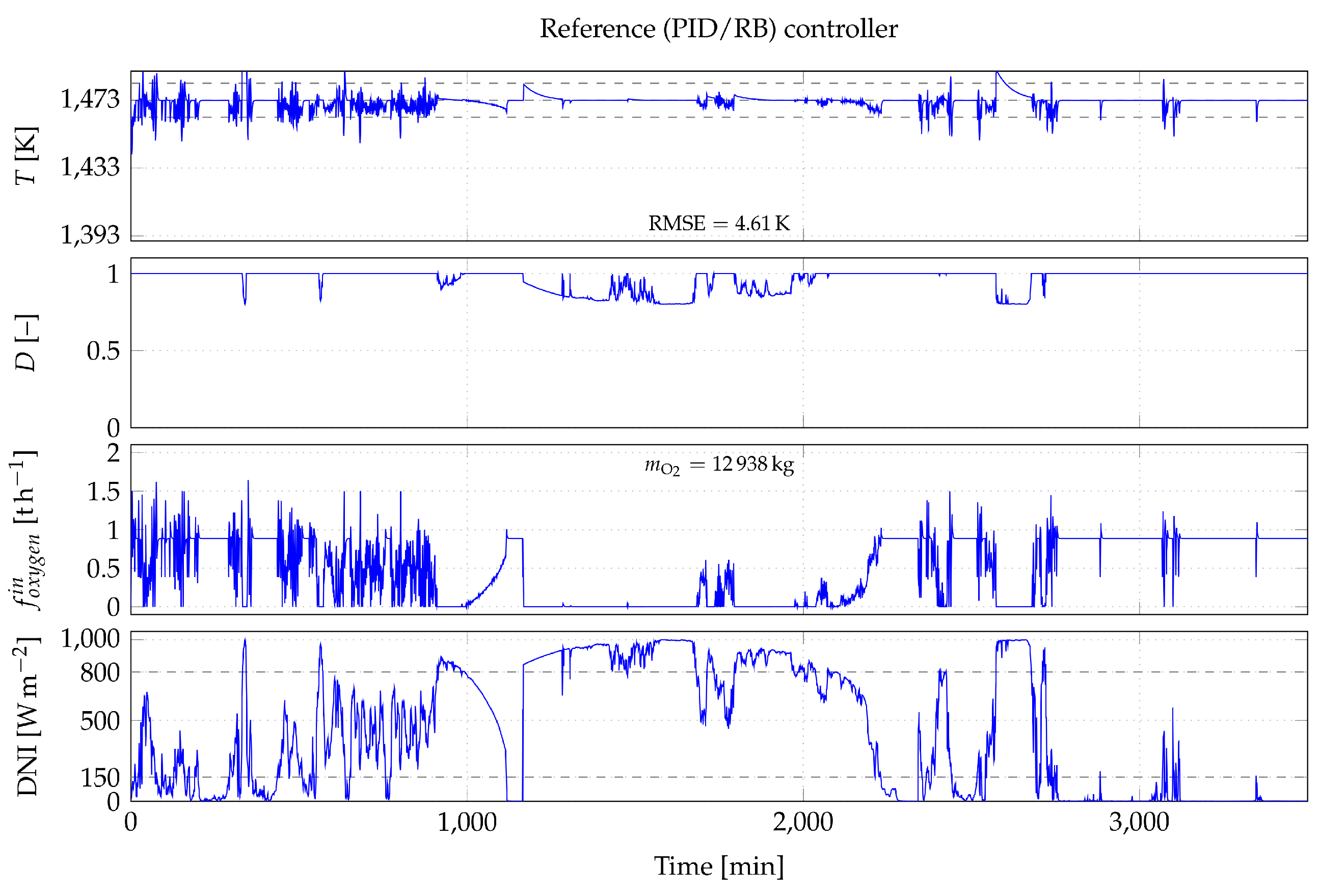
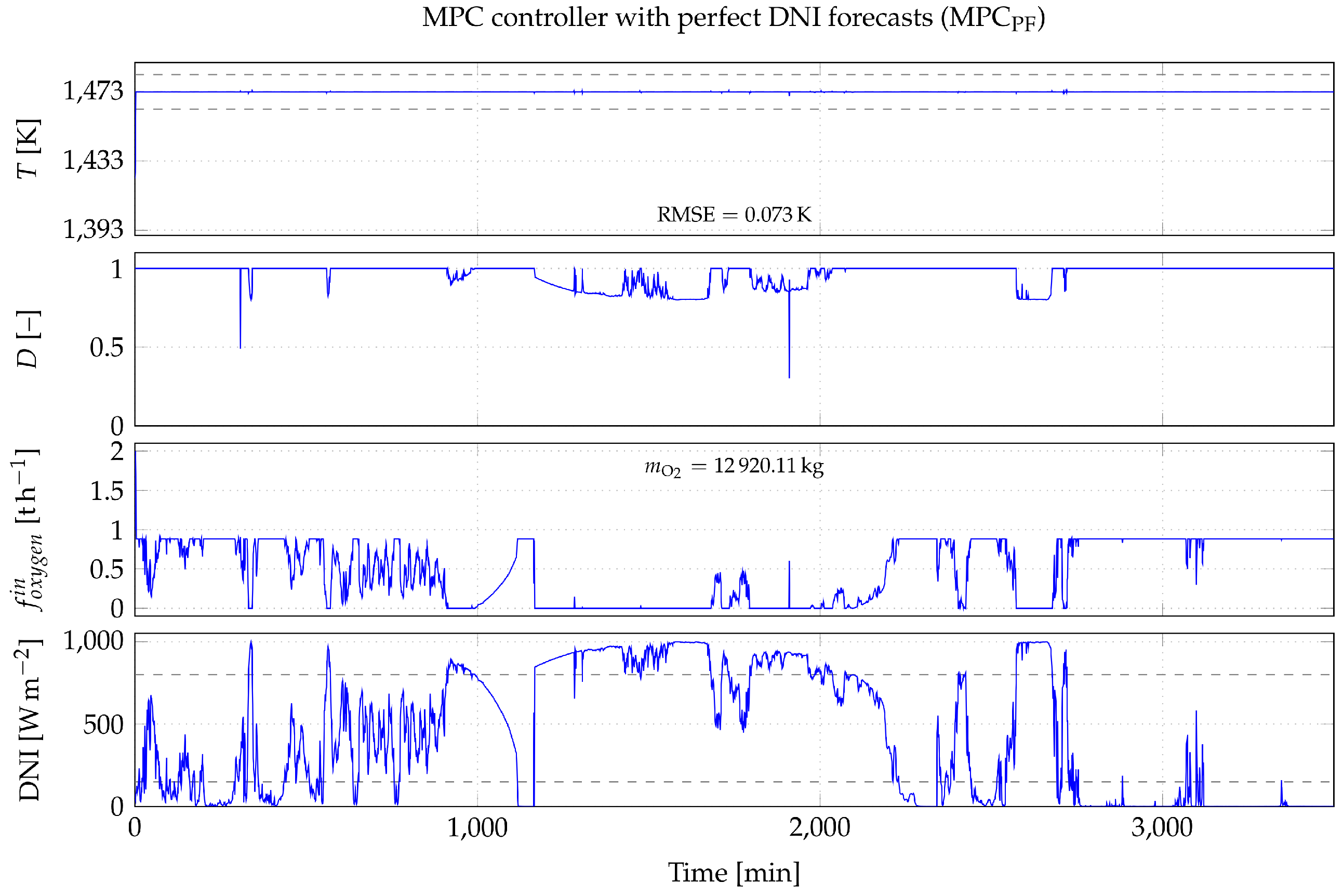
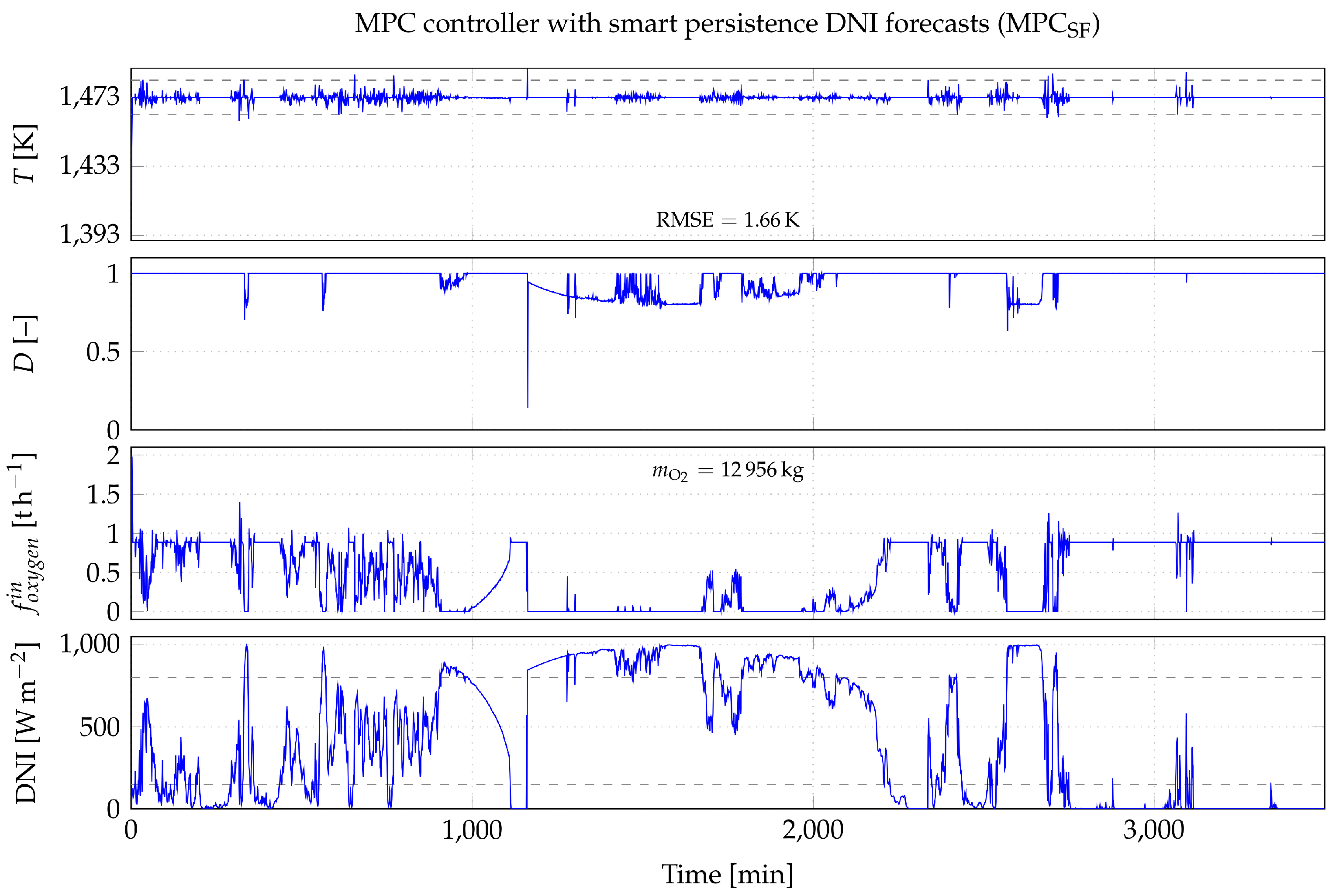
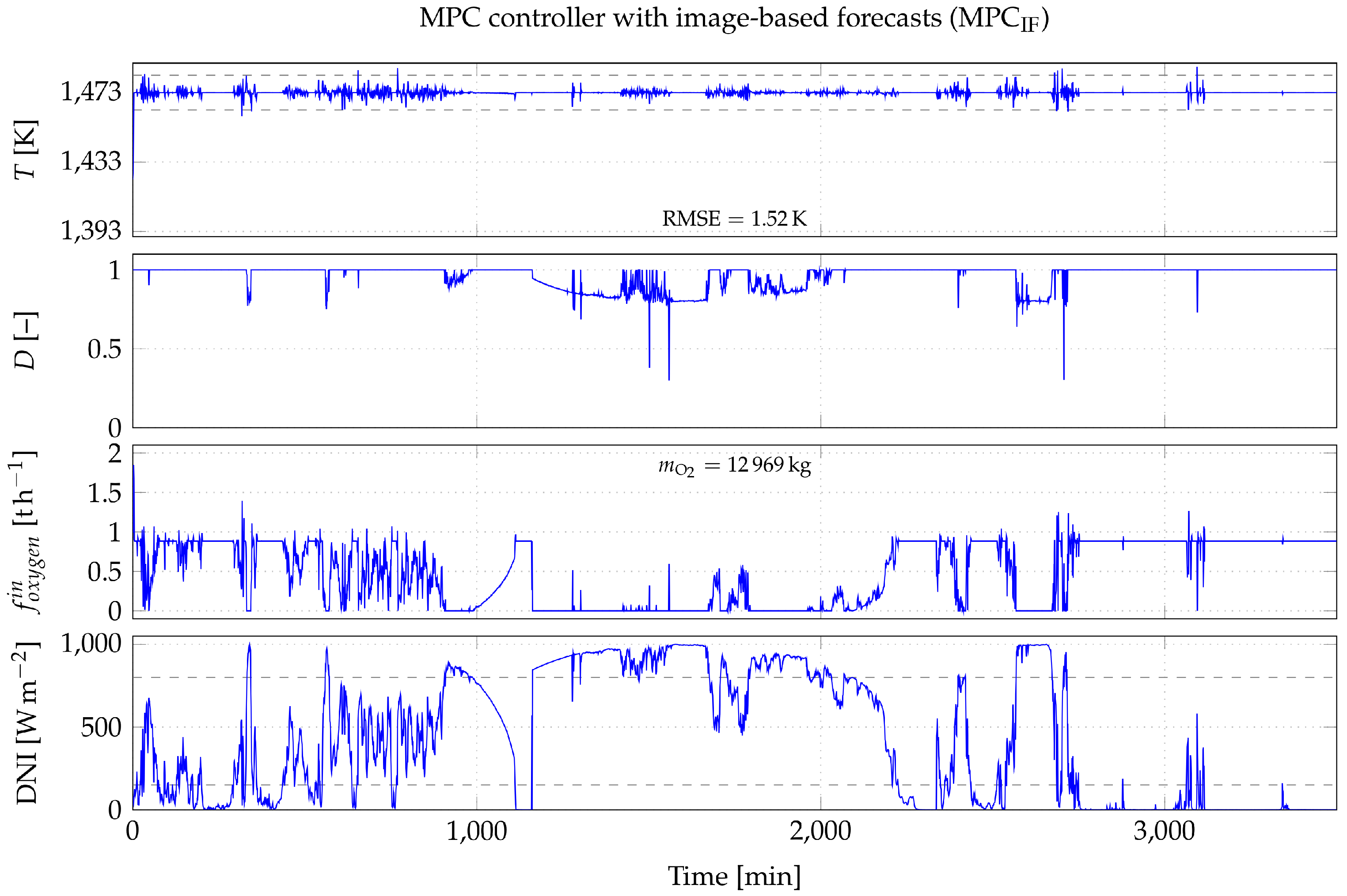
The main purpose of this case study is to gain some insight into the controllers’ behavior. Three days in the test dataset are considered because DNI is highly variable, with clear-sky, overcast, and mixed situations. Night-time periods are not included, since they are identical to the case where $\mathrm{DNI}<150 \mathrm{W}{\mathrm{m}}^{-2}$: injecting $0.88 \mathrm{t}{\mathrm{h}}^{-1}$ of oxygen is sufficient to perfectly maintain the reactor’s temperature. Figure 15, Figure 16, Figure 17 and Figure 18 display several plots against time: the reactor’s temperature T, the defocusing factor D, the oxygen flow rate $f_{oxygen}^{in}$, and the measured DNI, from top to bottom. As can be seen, the reference (PID/RB) controller (Figure 15) is able to maintain the reactor’s temperature at its nominal value but is very sensitive to DNI variations. This controller is able to operate for the three intervals of DNI values ($\mathrm{DNI}<150 \mathrm{W}{\mathrm{m}}^{-2}$, $150\mathrm{W}{\mathrm{m}}^2⩽\mathrm{DNI}⩽800 \mathrm{W}{\mathrm{m}}^{-2}$ and $\mathrm{DNI}>800 \mathrm{W}{\mathrm{m}}^{-2}$), thanks to its adaptive nature. When the reactor’s aperture is closed, the reactor’s temperature is maintained perfectly, as shown from 100 min to 150 min. In case of an excess of DNI, from 150 min to 200 min for example, the mirror’s controller adjusts the defocusing factor D to maintain the reactor’s temperature by eliminating this excess. Needless to say, in this case, the injection of oxygen is minimal. Finally, the controller provides acceptable performance when DNI varies between 150 $\mathrm{W}{\mathrm{m}}^{-2}$ and 800 $\mathrm{W}{\mathrm{m}}^{-2}$. Although the controller is able to correctly manage the solar reactor, variations of its temperature are important: RMSE is $4.61$ K over the simulation period. Regarding the MPC controller, perfect DNI forecasts are first provided (${MPC}_{\mathrm{PF}}$) to showcase the MPC optimal performance (Figure 16). The controller is able to maintain the reactor’s temperature, scoring a low RMSE of $0.073$ K while injecting 12,920.11 kg of oxygen ($m_{{\mathrm{O}}_2}$= 12,938 kg for the reference controller). The controller tends to tilt the concentration mirrors only in case of an excess of DNI, which aims to maximize the amount of solar energy received by the reactor, thus reducing the consumption of oxygen. In case of smart persistence DNI forecasts (${MPC}_{\mathrm{SF}}$), the controller is able to maintain the reactor’s temperature, scoring an RMSE of $1.66$ K (vs. $0.073$ K for the MPC controller with perfect DNI forecasts and $4.61$ K for the reference controller); however, some fluctuations can be observed due to inaccurate forecasts (Figure 17). Oxygen consumption is 12,956 kg (vs. 12,920.11 kg for the MPC controller with perfect DNI forecasts and 12,938 kg for the reference controller). The controller is able to function properly in the closed-reactor scenario and around it ($\mathrm{DNI}<150 \mathrm{W}{\mathrm{m}}^{-2}$) by injecting the right amount of oxygen ($0.88 \mathrm{t}{\mathrm{h}}^{-1}$). The excess of DNI is compensated by defocusing the concentration mirrors. The controller tends to defocalize the mirrors to compensate for strong DNI variations as well, thus wasting solar energy to maintain the reactor’s temperature accurately. Finally, the results provided by the MPC controller with image-based DNI forecasts (${MPC}_{\mathrm{IF}}$) are shown in Figure 18. The controller is able to maintain the reactor’s temperature, scoring an RMSE of $1.52$ K (vs. $0.073$ K for the MPC controller with perfect DNI forecasts and $4.61$ K for the reference controller); however, some fluctuations can be observed due to DNI ramps not detected using the sky images. Oxygen consumption is 12,969 kg (vs. 12,920.11 kg for the MPC controller with perfect DNI forecasts and 12,938 kg for the reference controller). Again, the controller is able to function properly in the closed-reactor scenario ($\mathrm{DNI}<150 \mathrm{W}{\mathrm{m}}^{-2}$) by injecting the right amount of oxygen ( $0.88 \mathrm{t}{\mathrm{h}}^{-1}$), the excess of DNI being compensated by defocusing the concentration mirrors. It should be noted that whatever the controller, oxygen consumption is more or less the same.

6. Computationally-Tractable MPC Controller

The high optimization time is due to the Cantera function, which takes on average $0.05$ s to calculate $Q_{reaction}$ for one time step (see Table 4). As a result, for the optimization problem to be solved quickly at each time step, the model used by the MPC controller should be computationally tractable and $Q_{reaction}$ calculated faster. That is why replacing the Cantera function with a 2D interpolation function is proposed here; then, the robustness of the MPC controller to the model simplification is evaluated. Let us note that such a simplification impacts on the optimal prediction horizon of the MPC controller.

6.1. Model Simplification

The reaction power $Q_{reaction}$ is calculated for a given temperature and reactant flow rates (biomass, steam, and oxygen) using the Cantera toolbox. Since the biomass and steam flow rates are fixed to their nominal values, the toolbox could be replaced with a function that takes the current reactor’s temperature and the oxygen flow rate as input and computes $Q_{reaction}$. After analyzing the influence of the reactor’s temperature and the oxygen flow rate on $Q_{reaction}$ (Figure 19), it can be observed that:

• for a given reactor’s temperature, $Q_{reaction}$ is mainly a linear function of the oxygen flow rate (0 th${}^{-1}$$⩽f_{oxygen}^{in}⩽1.8$ th${}^{-1}$);
• for a given oxygen flow rate, $Q_{reaction}$ is a linear function of the reactor’s temperature ($1453 \mathrm{K}⩽T⩽1493 \mathrm{K}$).

The chosen neighborhood is around the nominal performance (1453 K $⩽T⩽$ 1493 K) while respecting the oxygen flow rate constraint (0 th${}^{-1}$$⩽f_{oxygen}^{in}⩽$ 1.8 th${}^{-1}$). This approach is tested on 545,232 combinations (not included in the interpolation database), and the resulting mean absolute error (MAE) between the output of the 2D interpolation function and the Cantera function is 2.14 kW, which induces an error of 0.01 K on temperature variations. This low MAE and this fast execution time justify the replacement of the Cantera function with an interpolation function to solve the optimization problem. Let us note that the original model $\mathcal{M}$ is still used to perform the simulation when applying the optimal inputs, i.e., the defocusing factor D and the oxygen flow rate $f_{oxygen}^{in}$ (Figure 20).

6.2. MPC Controller with Simplified Reactor Model vs. MPC Controller with Original Reactor Model

Table 5. MPC evaluation: simplified reactor model vs. original reactor model $\mathcal{M}$ for the three types of DNI forecasts (7-day simulation). RMSE is the root mean squared error. $m_{{\mathrm{O}}_2}$ is the amount of oxygen injected in the reactor. ATV is the average temperature variation. $f_{obj}$ is the objective function value. ${\tau }_{opt}$ is the mean optimization time per time step.

Controller	Performance Criterion	Prediction Horizon of the MPC Controller (min)
		0.5	1	1.5	2	2.5
${MPC}_{\mathrm{PF}}$ with simplified reactor model	RMSE (K)	0.49	0.10	0.10	0.11	0.11
	$m_{{\mathrm{O}}_2}$ (kg)	31,956	31,961	31,965	31,972	31,979
	$\mathrm{ATV}$ (K)	0.04	0.05	0.05	0.05	0.05
	$f_{obj}$	−40,831.19	−48,508.93	−48,500.45	−48,493.56	−48,487.42
	${\tau }_{opt}$ (s)	0.1	0.2	0.3	0.4	0.5
${MPC}_{\mathrm{PF}}$ with original reactor model $\mathcal{M}$	RMSE (K)	0.451	0.073	0.075	0.078	0.078
	$m_{{\mathrm{O}}_2}$ (kg)	31,945.55	31,968.33	31,964.17	31,988.02	31,959.63
	$\mathrm{ATV}$ (K)	0.018	0.031	0.032	0.034	0.036
	$f_{obj}$	−42,139.13	−48,657.01	−48,653.24	−48,549.71	−48,559.12
	${\tau }_{opt}$ (s)	1.5	5	10	15	30
${MPC}_{\mathrm{SF}}$ with simplified reactor model	RMSE (K)	2.01	1.97	1.74	1.73	1.74
	$m_{{\mathrm{O}}_2}$ (kg)	32,043	32,093	32,137	32,152	32,106
	$\mathrm{ATV}$ (K)	1.60	1.50	1.50	1.49	1.50
	$f_{obj}$	85,065.71	80,101	51,807	51,350	51,652.50
	${\tau }_{opt}$ (s)	0.1	0.2	0.3	0.4	0.5
${MPC}_{\mathrm{SF}}$ with original reactor model $\mathcal{M}$	RMSE (K)	1.92	1.79	1.71	1.72	1.71
	$m_{{\mathrm{O}}_2}$ (kg)	32,080.55	32,074.03	32,089.23	32,075.459	32,090
	$\mathrm{ATV}$ (K)	1.50	1.47	1.542	1.58	1.47
	$f_{obj}$	74,260.74	56,858.36	48,620.45	49,702.90	48,638.47
	${\tau }_{opt}$ (s)	1	4.6	9.7	14.5	29
${MPC}_{\mathrm{IF}}$ with simplified reactor model	RMSE (K)	1.97	1.89	1.64	1.62	1.63
	$m_{{\mathrm{O}}_2}$ (kg)	32,102	32,081	32,114	32,126	32,146
	$\mathrm{ATV}$ (K)	3.10	1.47	1.47	1.47	1.47
	$f_{obj}$	80,943	69,440	41,032.92	38,072	40,028
	${\tau }_{opt}$ (s)	0.1	0.2	0.3	0.4	0.5
${MPC}_{\mathrm{IF}}$ with original reactor model $\mathcal{M}$	RMSE (K)	1.88	1.72	1.64	1.60	1.61
	$m_{{\mathrm{O}}_2}$ (kg)	32,142	32,058.87	32,063.25	32,091.25	32,143.56
	$\mathrm{ATV}$ (K)	3.00	1.45	1.46	1.47	1.47
	$f_{obj}$	68,903	49,334.44	40,786.92	36,446.05	37,996.54
	${\tau }_{opt}$ (s)	1.5	5	10	15	30

deals with evaluating the robustness of the controller to possible uncertainties resulting from model simplification. The MPC controller with a simplified reactor model is compared to the same controller with the original reactor model (see Table 4) for the three types of DNI forecasts (perfect forecasts, smart persistence forecasts and image-based forecasts). The results show that the MPC controller with the simplified reactor model is robust to possible uncertainties resulting from model simplification as long as the controller is able to maintain the reactor’s temperature while minimizing oxygen consumption: for ${MPC}_{\mathrm{PF}}$ and a prediction horizon of $2.5$ min, switching from the original model to the simplified model decreases the mean optimization time per time step ${\tau }_{opt}$ from $30 \mathrm{s}$ to $0.5 \mathrm{s}$, for an increase of RMSE from $0.08$ K to $0.11$ K. For ${MPC}_{\mathrm{SF}}$ and a prediction horizon of $1.5$ min, switching from the original model to the simplified model decreases ${\tau }_{opt}$ from $9.7 \mathrm{s}$ to $0.3 \mathrm{s}$ for an increase of RMSE from $1.71$ K to $1.74$ K. Regarding the MPC controller with image-based forecasts (${MPC}_{\mathrm{IF}}$), it still manages to score lower RMSE and uses less oxygen than with smart persistence forecasts, which highlights the importance of accurate DNI forecasts (and, as a result, the use of sky images), even when the simplified reactor model is used (RMSE is $1.63$ K for a prediction horizon of 2.5 min). In terms of computational complexity, using the simplified reactor model reduces the mean optimization time per time step drastically (up to 58 times for a prediction horizon of 2.5 min).

6.3. MPC Controller with Simplified Reactor Model vs. Reference Controller

The MPC controller with a simplified reactor model—the optimal prediction horizon is 1 min for ${MPC}_{\mathrm{PF}}$ and 2 min for ${MPC}_{\mathrm{SF}}$ and ${MPC}_{\mathrm{IF}}$—can be compared to the reference (PID/RB) controller: even when the simplified reactor model is used, the MPC controller still manages to outperform the reference controller by scoring lower RMSE—RMSE (PID/RB) is $4.88$ K whereas RMSE (${MPC}_{\mathrm{SF}}$) is $1.73$ K and RMSE (${MPC}_{\mathrm{IF}}$) is $1.62$ K—and ATV—ATV (PID/RB) is $2.27$ K whereas ATV (${MPC}_{\mathrm{SF}}$) is $1.49$ K and ATV (${MPC}_{\mathrm{IF}}$) is $1.47$ K—values at the cost of an increase of less than 0.01% in oxygen consumption.

7. Conclusions

This paper deals with the modeling and dynamic control of a solar hybrid thermochemical reactor that uses concentrated solar energy to produce syngas through the high-temperature steam gasification of biomass. A model-based predictive controller is proposed and compared to a reference controller which consists of an adaptive PID controller (for the oxygen flow rate) with optimized gains and a rule-based controller (for the defocusing factor). The ultimate goal of these controllers is to maintain the reactor’s temperature at its nominal value despite DNI variations, thus ensuring the reactor’s stability. Different DNI forecasts are provided to the MPC controller: perfect forecasts, smart persistence forecasts, and image-based forecasts, where the model processes HDR sky images to forecast DNI by anticipating possible DNI variations (DNI ramps). The MPC controller, which is able to find a trade-off between maintaining the reactor’s temperature and minimizing oxygen consumption while exploiting the available solar energy, manages to outperform the reference controller by scoring lower RMSE and ATV values at the cost of an increase in oxygen consumption of less than 0.5% with all DNI forecasts. In addition, the integration of image-based forecasts results in better performance, and replacing the Cantera function with a 2D interpolation function allows a significant reduction in optimization time at the cost of a slight performance degradation. More sophisticated control strategies could be now developed, for example a strategy focusing on maximizing the production of syngas, while ensuring the reactor’s stability. Different control inputs could be used: for example, the biomass flow rate can compensate for DNI variations. For implementing these strategies, the reactor model should account for the kinetics of the biomass gasification reaction as well.

References

1. Gregg, D.; Taylor, R.; Campbell, J.; Taylor, J.; Cotton, A. Solar gasification of coal, activated carbon, coke and coal and biomass mixtures. Sol. Energy 1980, 25, 353–364. [Google Scholar] [CrossRef]
2. Taylor, R.; Berjoan, R.; Coutures, J. Solar gasification of carbonaceous materials. Sol. Energy 1983, 30, 513–525. [Google Scholar] [CrossRef]
3. Yadav, D.; Banerjee, R. A review of solar thermochemical processes. Renew. Sustain. Energy Rev. 2016, 54, 497–532. [Google Scholar] [CrossRef]
4. Puig-Arnavat, M.; Tora, E.; Bruno, J.; Coronas, A. State of the art on reactor designs for solar gasification of carbonaceous feedstock. Sol. Energy 2013, 97, 67–84. [Google Scholar] [CrossRef]
5. Milanese, M.; Colangelo, G.; Iacobazzi, F.; de Risi, A. Modeling of double-loop fluidized bed solar reactor for efficient thermochemical fuel production. Sol. Energy Mater. Sol. Cells 2017, 160, 174–181. [Google Scholar] [CrossRef]
6. Gómez-Barea, A.; Suárez-Almeida, M.; Ghoniem, A. Analysis of fluidized bed gasification of biomass assisted by solar-heated particles. Biomass Convers. Biorefinery 2020, 11, 143–158. [Google Scholar] [CrossRef]
7. Bellouard, Q.; Abanades, S.; Rodat, S. Biomass Gasification in an Innovative Spouted-Bed Solar Reactor: Experimental Proof of Concept and Parametric Study. Energy Fuels 2017, 31, 10933–10945. [Google Scholar] [CrossRef]
8. Boujjat, H.; Rodat, S.; Chuayboon, S.; Abanades, S. Experimental and numerical study of a directly irradiated hybrid solar/combustion spouted bed reactor for continuous steam gasification of biomass. Energy 2019, 189, 116118. [Google Scholar] [CrossRef]
9. Curcio, A.; Rodat, S.; Vuillerme, V.; Abanades, S. Experimental assessment of woody biomass gasification in a hybridized solar powered reactor featuring direct and indirect heating modes. Int. J. Hydrog. Energy 2021, 46, 37192–37207. [Google Scholar] [CrossRef]
10. Muroyama, A.P.; Guscetti, I.; Schieber, G.L.; Haussener, S.; Loutzenhiser, P.G. Design and demonstration of a prototype 1.5 kWth hybrid solar/autothermal steam gasifier. Fuel 2018, 211, 331–340. [Google Scholar] [CrossRef] [Green Version]
11. Hathaway, B.J.; Davidson, J.H. Autothermal hybridization and controlled production of hydrogen-rich syngas in a molten salt solar gasifier. Int. J. Hydrog. Energy 2021, 46, 15257–15267. [Google Scholar] [CrossRef]
12. Blanc, P.; Espinar, B.; Geuder, N.; Gueymard, C.; Meyer, R.; Pitz-Paal, R.; Reinhardt, B.; Renné, D.; Sengupta, M.; Wald, L.; et al. Direct normal irradiance related definitions and applications: The circumsolar issue. Sol. Energy 2014, 110, 561–577. [Google Scholar] [CrossRef]
13. Maffezzoni, C.; Parigi, F. Dynamic analysis and control of a solar power plant—II. Control system design and simulation. Sol. Energy 1982, 28, 117–128. [Google Scholar] [CrossRef]
14. Camacho, E.; Rubio, F.; Hughes, F. Self-tuning control of a solar power plant with a distributed collector field. IEEE Control. Syst. 1992, 12, 72–78. [Google Scholar] [CrossRef]
15. Rubio, F.; Berenguel, M.; Camacho, E. Fuzzy logic control of a solar power plant. IEEE Trans. Fuzzy Syst. 1995, 3, 459–468. [Google Scholar] [CrossRef]
16. Pickhardt, R. Nonlinear modelling and adaptive predictive control of a solar power plant. Control. Eng. Pract. 2000, 8, 937–947. [Google Scholar] [CrossRef]
17. Arahal, M.; Berenguel, M.; Camacho, E. Neural identification applied to predictive control of a solar plant. Control. Eng. Pract. 1998, 6, 333–344. [Google Scholar] [CrossRef]
18. Camacho, E.; Rubio, F.; Berenguel, M.; Valenzuela, L. A survey on control schemes for distributed solar collector fields. Part I: Modeling and basic control approaches. Sol. Energy 2007, 81, 1240–1251. [Google Scholar] [CrossRef]
19. Camacho, E.; Rubio, F.; Berenguel, M.; Valenzuela, L. A survey on control schemes for distributed solar collector fields. Part II: Advanced control approaches. Sol. Energy 2007, 81, 1252–1272. [Google Scholar] [CrossRef]
20. Petrasch, J.; Osch, P.; Steinfeld, A. Dynamics and control of solar thermochemical reactors. Chem. Eng. J. 2009, 145, 362–370. [Google Scholar] [CrossRef]
21. Saade, E.; Clough, D.E.; Weimer, A.W. Model predictive control of a solar-thermal reactor. Sol. Energy 2014, 102, 31–44. [Google Scholar] [CrossRef] [Green Version]
22. Muroyama, A.; Shinn, T.; Fales, R.; Loutzenhiser, P.G. Modeling of a Dynamically-Controlled Hybrid Solar/Autothermal Steam Gasification Reactor. Energy Fuels 2014, 28, 6520–6530. [Google Scholar] [CrossRef]
23. Boujjat, H.; Yuki Junior, G.M.; Rodat, S.; Abanades, S. Dynamic simulation and control of solar biomass gasification for hydrogen-rich syngas production during allothermal and hybrid solar/autothermal operation. Int. J. Hydrog. Energy 2020, 45, 25827–25837. [Google Scholar] [CrossRef]
24. Karout, Y.; Thil, S.; Eynard, J.; Guillot, E.; Grieu, S. Hybrid intrahour DNI forecast model based on DNI measurements and sky-imaging data. Sol. Energy 2023, 249, 541–558. [Google Scholar] [CrossRef]
25. Goodwin, D.G.; Speth, R.L.; Moffat, H.K.; Weber, B.W. Cantera: An Object-Oriented Software Toolkit for Chemical Kinetics, Thermodynamics, and Transport Processes. 2021. Available online: https://doi.org/10.5281/ZENODO.4527812 (accessed on 3 March 2021).
26. Curcio, A.; Rodat, S.; Vuillerme, V.; Abanades, S. Design and validation of reactant feeding control strategies for the solar-autothermal hybrid gasification of woody biomass. Energy 2022, 254, 124481. [Google Scholar] [CrossRef]
27. Dupont, C.; Boissonnet, G.; Seiler, J.M.; Gauthier, P.; Schweich, D. Study about the kinetic processes of biomass steam gasification. Fuel 2007, 86, 32–40. [Google Scholar] [CrossRef] [Green Version]
28. Smith, G.P.; Golden, D.M.; Frenklach, M.; Moriarty, N.W.; Eiteneer, B.; Goldenberg, M.; Bowman, C.T.; Hanson, R.K.; Song, S.; Gardiner, W.C.; et al. WHAT’S NEW IN GRI-Mech 3.0. Available online: http://combustion.berkeley.edu/gri-mech/version30/text30.html (accessed on 13 June 2021).
29. Ang, K.H.; Chong, G.; Li, Y. PID control system analysis, design, and technology. IEEE Trans. Control. Syst. Technol. 2005, 13, 559–576. [Google Scholar] [CrossRef] [Green Version]
30. Liu, G.; Daley, S. Optimal-tuning PID control for industrial systems. Control. Eng. Pract. 2001, 9, 1185–1194. [Google Scholar] [CrossRef]
31. García, C.E.; Prett, D.M.; Morari, M. Model predictive control: Theory and practice—A survey. Automatica 1989, 25, 335–348. [Google Scholar] [CrossRef]
32. Conn, A.R.; Gould, N.I.M.; Toint, P.L. Trust Region Methods; Society for Industrial and Applied Mathematics: Philadelphia, PA, USA, 2000. [Google Scholar] [CrossRef]
33. Martín, L.; Zarzalejo, L.F.; Polo, J.; Navarro, A.; Marchante, R.; Cony, M. Prediction of global solar irradiance based on time series analysis: Application to solar thermal power plants energy production planning. Sol. Energy 2010, 84, 1772–1781. [Google Scholar] [CrossRef]
34. Mishra, S.; Palanisamy, P. Multi-time-horizon solar forecasting using recurrent neural network. In Proceedings of the 2018 IEEE Energy Conversion Congress and Exposition (ECCE), Portland, OR, USA, 23–27 September 2018; pp. 18–24. [Google Scholar] [CrossRef] [Green Version]
35. Malakar, S.; Goswami, S.; Ganguli, B.; Chakrabarti, A.; Roy, S.S.; Boopathi, K.; Rangaraj, A.G. Designing a long short-term network for short-term forecasting of global horizontal irradiance. SN Appl. Sci. 2021, 3, 477. [Google Scholar] [CrossRef]
36. Brahma, B.; Wadhvani, R. Solar Irradiance Forecasting Based on Deep Learning Methodologies and Multi-Site Data. Symmetry 2020, 12, 1830. [Google Scholar] [CrossRef]
37. Du, J.; Min, Q.; Zhang, P.; Guo, J.; Yang, J.; Yin, B. Short-Term Solar Irradiance Forecasts Using Sky Images and Radiative Transfer Model. Energies 2018, 11, 1107. [Google Scholar] [CrossRef] [Green Version]
38. Chu, Y.; Pedro, H.T.C.; Coimbra, C.F.M. Hybrid intra-hour DNI forecasts with sky image processing enhanced by stochastic learning. Sol. Energy 2013, 98, 592–603. [Google Scholar] [CrossRef]
39. Quesada-Ruiz, S.; Chu, Y.; Tovar-Pescador, J.; Pedro, H.T.C.; Coimbra, C.F.M. Cloud-tracking methodology for intra-hour DNI forecasting. Sol. Energy 2014, 102, 267–275. [Google Scholar] [CrossRef]
40. Marquez, R.; Coimbra, C.F.M. Intra-hour DNI forecasting based on cloud tracking image analysis. Sol. Energy 2013, 91, 327–336. [Google Scholar] [CrossRef]
41. Caldas, M.; Alonso-Suárez, R. Very short-term solar irradiance forecast using all-sky imaging and real-time irradiance measurements. Renew. Energy 2019, 143, 1643–1658. [Google Scholar] [CrossRef]
42. Ineichen, P.; Perez, R. A new airmass independent formulation for the Linke turbidity coefficient. Sol. Energy 2002, 73, 151–157. [Google Scholar] [CrossRef] [Green Version]
43. Nou, J.; Chauvin, R.; Thil, S.; Grieu, S. A new approach to the real-time assessment of the clear-sky direct normal irradiance. Appl. Math. Model. 2016, 40, 7245–7264. [Google Scholar] [CrossRef] [Green Version]
44. Akiba, T.; Sano, S.; Yanase, T.; Ohta, T.; Koyama, M. Optuna: A Next-generation Hyperparameter Optimization Framework. In Proceedings of the Proceedings of the 25th ACM SIGKDD International Conference on Knowledge Discovery & Data Mining; Anchorage, AK, USA, 4–8 August 2019. [CrossRef]
45. Chu, Y.; Pedro, H.T.C.; Li, M.; Coimbra, C.F.M. Real-time forecasting of solar irradiance ramps with smart image processing. Sol. Energy 2015, 114, 91–104. [Google Scholar] [CrossRef]
Figure 1. PROMES-CNRS’s solar reactor prototype (Odeillo, France).
Cleantechnol 05 00018 g001
Figure 2. Evolution of the reactor’s temperature in response to various DNI steps (the biomass flow rate is set to f b i o m a s s i n = 1.465 th 1 and the initial temperature is 1073 K).
Cleantechnol 05 00018 g002
Figure 3. Power balance corresponding to the steady state of the DNI steps in Figure 2.
Cleantechnol 05 00018 g003
Figure 4. Reactor’s temperature in response to sudden DNI variations with nominal design values (T = 1473 K, DNI = 800   W m 2 and f b i o m a s s i n = 1.465   t h 1 ).
Cleantechnol 05 00018 g004
Figure 5. Evolution of the reactor’s temperature for various biomass flow rates when DNI is equal to 900   W m 2 and corresponding syngas production (dashed line: H2; solid line: H2 + CO).
Cleantechnol 05 00018 g005
Figure 6. Syngas (H2 + CO) production for various oxygen flow rates and DNI levels.
Cleantechnol 05 00018 g006
Figure 7. Evolution of the reactor’s temperature for various oxygen flow rates and DNI levels ( f b i o m a s s i n = 1.465 th 1 and the initial temperature is 1073 K).
Cleantechnol 05 00018 g007
Figure 8. Evolution of the reactor’s temperature in case of a closed aperture and an oxygen flow rate f o x y g e n i n = 0.88 th 1 ( f b i o m a s s i n = 1.465 th 1 , and the initial temperature is 1073 K).
Cleantechnol 05 00018 g008
Figure 9. The reference controller, defined as a combination of an adaptive PID controller with optimized gains (for the oxygen flow rate f o x y g e n i n ) and a rule-based controller (for the defocusing factor D).
Cleantechnol 05 00018 g009
Figure 10. The MPC controller. The optimizer used is the trust-region constrained algorithm [32].
Cleantechnol 05 00018 g010
Figure 11. Left: The sky imager installed at the PROMES-CNRS laboratory in Odeillo (France). Right: A high-dynamic-range (HDR) sky image, without correction of the distortion.
Cleantechnol 05 00018 g011
Figure 12. High-dynamic-range (HDR) sky images and associated sky situations: clear sky, overcast and mixed. Days with mixed situations can be partially clear sky or partially overcast.
Cleantechnol 05 00018 g012
Figure 13. Global architecture of the proposed forecast model, showing two main blocks: image processing and DNI forecasting. CF ROI H is the cloud fraction in the ROI. The interested reader is referred to [24] for details about the image processing block.
Cleantechnol 05 00018 g013
Figure 14. Image-based model results: RMSE, SF, MAE, and RDI as a function of the forecast horizon H (test phase).
Cleantechnol 05 00018 g014
Figure 15. Case study results: reference (PID/RB) controller.
Cleantechnol 05 00018 g015
Figure 16. Case study results: MPC controller with perfect DNI forecasts ( MPC PF ). The prediction horizon of the controller is 1 min.
Cleantechnol 05 00018 g016
Figure 17. Case study results: MPC controller with smart persistence DNI forecasts ( MPC SF ). The prediction horizon of the controller is 1.5 min.
Cleantechnol 05 00018 g017
Figure 18. Case study results: MPC controller with image-based DNI forecasts ( MPC IF ). The prediction horizon of the controller is 2 min.
Cleantechnol 05 00018 g018
Figure 19. Power resulting from the gasification reaction as a function of oxygen flow rate variations (left) and reactor’s temperature variations (right).
Cleantechnol 05 00018 g019
Figure 20. The computationally tractable MPC controller. The orignial reactor model M is replaced with the simplified model to solve the optimization problem. The original model M is still used to perform the simulation.
Cleantechnol 05 00018 g020