Article

Salinity of Irrigated and Non-Irrigated Chernozems and Kastanozems: A Case Study of Causes and Consequences in the Pavlodar Region, Kazakhstan

by
Dauren Rakhmanov
1,2,
Bořivoj Šarapatka
1,*,
Marek Bednář
1,
Jan Černohorský
1 and
Kamilla Alibekova
1
1
Department of Ecology and Environmental Sciences, Palacký University, 17. listopadu 12, 771 46 Olomouc, Czech Republic
2
Department of Agrotechnology, Toraighyrov University, Lomov 64, Pavlodar 140008, Kazakhstan
*
Author to whom correspondence should be addressed.
Soil Syst. 2025, 9(2), 57; https://doi.org/10.3390/soilsystems9020057
Submission received: 18 March 2025 / Revised: 20 May 2025 / Accepted: 22 May 2025 / Published: 28 May 2025
(This article belongs to the Special Issue Research on Soil Management and Conservation: 2nd Edition)

Abstract

This study investigated soil salinization processes in the Pavlodar region of Kazakhstan by comparing key soil parameters—namely, electrical conductivity (EC), pH, exchangeable sodium percentage (ESP), and sodium adsorption ratio (SAR) under irrigated and non-irrigated conditions across different agro-climatic zones and soil types (Haplic Chernozems, Haplic Kastanozems). The focus was on understanding the effects of irrigation and natural factors on soil salinization. Statistical analysis, including descriptive statistics and significance testing, was employed to evaluate differences between soil types, locations, and management practices. The research revealed secondary salinization (EC > 2 dS/m, ESP > 15%) in the topsoil of irrigated Haplic Kastanozems soils in the central Aksu district. This degradation was markedly higher than in non-irrigated plots or irrigated Haplic Chernozems in the northern Irtysh district, highlighting the high vulnerability of Haplic Kastanozems soils under current irrigation management given Aksu’s climatic conditions, which are characterized by high evaporative demand (driven by summer temperatures) and specific precipitation patterns that contribute to soil moisture deficits without irrigation. While ESP indicated sodicity, SAR values remained low. Natural factors, including potentially saline parent materials and likely shallow groundwater dynamics influenced by irrigation, appear to contribute to the observed patterns. The findings underscore the need for implementing optimized irrigation and drainage management, particularly in the Aksu district, potentially including water-saving techniques (e.g., drip irrigation) and selection of salt/sodicity-tolerant crops. A comprehensive approach integrating improved water management, agronomic practices, and potentially soil amendments is crucial for mitigating soil degradation and ensuring sustainable agriculture in the Pavlodar region. Further investigation including groundwater monitoring is recommended.

1. Introduction

In order to feed the global human population, which will reach 8.5 billion by 2030, agricultural production must first be increased in a sustainable manner. This growth in world crop production expected for the year 2030 is to be achieved with 87 percent through increased productivity, 6 percent through area expansion, and 7 percent through increased agricultural intensity [1]. Solving these problems also includes irrigation, as only 20% of the world’s arable land produces 40% of the world’s crop production, meaning that irrigation more than doubles land productivity. In arid and semi-arid regions, proper irrigation increases economic returns and can increase production by up to 400%. On the other hand, irrigation can lead to undesirable consequences for the environment. About a third of the world’s irrigated land has lost productivity due to irrigation mismanagement, leading to secondary salinization of agricultural land [2].
Secondary salinization happens when excessive irrigation is used without proper drainage, causing the groundwater level to rise. Currently, secondary salinization is a significant problem for the security of arid ecosystems [1]. Soil salinity depends on several factors, namely soil, water quality, local topography, climatic factors, and above all improper management, especially in arid regions [3,4,5]. Soil salinization is recognized globally as a serious environmental issue due to its detrimental impact on soil health and productivity [6]. Unsuitable agricultural activities—such as improper irrigation methods, overuse of agrochemicals, and lack of soil conservation—can exacerbate salinity and accelerate soil erosion. This in turn leads to loss of fertile land, reduction in soil resources, decreased crop yields, nutrient depletion, and shrinkage of cultivated areas [7,8]. Soil salinization also has an indirect effect, leading to loss of soil stability due to changes in soil structure [9]. Additionally, leaching of salts from soil can easily cause saline water to negatively affect groundwater [10]. In a study by Ibraeva et al. [11], it was noted that when salt concentrations exceed 0.05%, the number of ammonifiers, nitrogen fixers, and nitrifiers decreases, which can negatively affect the nitrogen cycle in soils. In contrast, denitrifying bacteria and microscopic fungi do not respond to increased salt levels. However, overall soil salinization inhibits the growth of nitrogen-fixing and sulfate-reducing bacteria.
Currently, up to 40–60% of irrigated land in Central Asia is prone to salinity or waterlogging [12,13]. The World Resources Institute reports that in the last 50 years, approximately 66% of agricultural land has experienced varying levels of degradation due to factors such as erosion, salinization, nutrient loss, compaction, biological decline, or pollution. Also, according to the Food and Agriculture Organization, about one-tenth of the world’s irrigated land suffers from soil salinization, which could threaten 10% of the world’s grain harvest [14].
In general, soil salinization has a negative impact on agriculture, reducing crop yields and deteriorating their quality [15]. This leads to economic losses for farmers and the region as a whole. Environmental impacts include land degradation, loss of biodiversity, and deterioration of water quality. The socio-economic consequences are manifested in a decrease in the standard of living of the population employed in agriculture and in an increase in the cost of restoring soil fertility [16].
The Pavlodar region, which is located in the northeastern part of Kazakhstan, also faces this problem to a large extent. The natural conditions of northern Kazakhstan and the energy potential of the soils in this zone indicate the efficiency of agriculture, especially with irrigated soils [17]. While the Pavlodar region also includes areas of naturally salt-affected soils, such as Solonetz, agricultural activities are predominantly concentrated in Chernozems and Kastanozems types [18]. Therefore, these dominant agricultural soil types were chosen for this study.
The main objectives of this study were as follows:
  • To compare key soil salinity parameters (EC, pH, SAR, and ESP) within the studied soil profile (0–100 cm) of dominant agricultural soils (Haplic Chernozems, Haplic Kastanozems) under irrigated and non-irrigated conditions within three contrasting agro-climatic districts (Irtysh, Aksu, and Maysky) of the Pavlodar region, Kazakhstan;
  • To assess the differences in salinity levels between the studied soil types and districts, considering their distinct climatic conditions and management practices;
  • To evaluate the vertical distribution patterns of salts within the studied soil profiles.

2. Materials and Methods

2.1. Study Area

The Pavlodar region, located in the northeastern part of Kazakhstan (Figure 1), spans over 450 km from west to east (73°30′ to 80° E) and over 500 km from south to north (50° to 54°30′ N) [19]. The region exhibits significant natural diversity, primarily encompassing steppe and desert–steppe natural zones. The overall relief is predominantly a flat to gently undulating plain of the West Siberian Lowland and adjacent Kazakh Uplands, featuring the wide Irtysh River Valley. Groundwater levels within the Irtysh Valley vary with geomorphic position, ranging from 1 to 2 m in the near-channel floodplain and from 1.5 to 2.5 m in the central floodplain and from 3 to 4 m or deeper on the high floodplain terrace [18,19].
The region’s climate transitions from north to south [20], influencing vegetation and soil types. The average annual air temperature ranges from 2.3 °C in the north to 3.9 °C in the south, with warm summers (July average 20.3–21.9 °C) and cold winters (January average −17.4 to −12.8 °C). Precipitation also decreases southwards.
This climatic gradient governs the distribution of major soil types and natural vegetation. Following internationally recognized classification systems [21], the main soils studied are the following:
Southern Chernozems (Haplic Chernozems, WRB): Common in the northern part of the region (north of approx. 53°20′ N), typically forming under forb-grass steppe vegetation on relatively higher-relief elements outside the main river floodplain. Compared to European Chernozems, they have a shallower humus horizon and often exhibit slight inherent sodicity [19].
Dark Chestnut Soils (Haplic Kastanozems, WRB): Predominant in the middle zone, developing under dry fescue-feather grass steppe. They show considerable diversity due to variable parent materials, and sodic variants are common [19].
Light Chestnut Soils (Haplic Kastanozems, WRB): Found in the climatically extreme south (south of approx. 50°40′ N, Maysky district), often in association with semi-desert wormwood–grass communities. Their development was strongly influenced by saline marine deposits underlying the area, contributing to the natural prevalence of soil salinity [19]. This results in a complex soil cover where agriculture, especially under irrigation, interacts with these inherent soil properties, hydrogeological conditions, and regional climatic factors. The Department of Land Relations in the Pavlodar region reports that agricultural lands account for 89.5% of the region’s total land area. This includes a significant amount of pastureland, totaling 8229.5 thousand hectares (Figure 2), and arable land, which covers 1569.1 thousand hectares. Additionally, fallow lands exceed 1 million hectares [22].

2.2. Collection of Soil Samples and Their Chemical Analysis

To analyze the soil characteristics under different conditions within the Pavlodar region, three key districts—Irtysh, Aksu, and Maysky—were purposively selected for this study. These districts represent a characteristic north-to-south agro-climatic transect across the region, allowing for the investigation of the region’s dominant agricultural soil types under varying climatic conditions and management practices:
The Irtysh district, located in the northern, more humid part of the region, is known for its Haplic Chernozems, characterized by high fertility and significant humus content.
The Aksu district, situated in the central part, features Haplic Kastanozems, which typically have a less pronounced humus layer compared to Haplic Chernozems.
The Maysky district, in the drier, southern part of the region, is characterized by Haplic Kastanozems, usually lighter in color and with different structural features.
Within each of these three districts, sampling focused on areas under active agricultural use to assess the impact of management. To enable a direct comparison of irrigation effects, paired study sites were chosen: one representative field under long-term irrigation (predominantly sprinkler irrigation using center pivot systems) and an adjacent or nearby non-irrigated field under similar basic agricultural management.
Soil samples were collected from both irrigated and non-irrigated agricultural areas across the three study districts (Irtysh, Aksu, and Maysky) to assess the difference in their properties and condition. The study encompassed six experimental plots (each larger than 1 ha), representing both management types (one plot per district/irrigation combination). The irrigated plots typically utilized sprinkler irrigation, particularly center pivot systems fed by open irrigation canals originating from the Irtysh River and the Irtysh–Karaganda canal system. Non-irrigated lands relied solely on natural precipitation, making their crop yields more vulnerable to climatic fluctuations [23].
Field sampling for this comparative study was conducted in 2023, immediately following the harvest of the primary crop. This post-harvest timing was chosen because previous studies indicated that this period typically corresponds to when the highest level of salt accumulation is observed in the topsoil, allowing for assessment of cumulative seasonal effects [23]. According to regional meteorological data, the weather conditions during the preceding growing season in 2023 and at the time of sampling were broadly typical for the long-term average.
Within each of the six plots, soil sampling was carried out with five-fold replication for each of the three investigated soil depths: 0–20 cm (I layer), 21–50 cm (II layer), and 51–100 cm (III layer). To obtain each single replicate composite sample for a specific depth, the envelope sampling pattern was employed. This involved collecting multiple soil sub- samples from five points within the plot (four corners and the center) at the target depth. Specifically, at each of these five points, five individual scoops/cores (sub-samples) were taken and combined (totaling 5 points × 5 scoops/point = 25 scoops per replicate). These collected sub-samples were then thoroughly mixed to create one replicate composite sample. This entire procedure was repeated for all five replicates at each specific depth within each plot. Therefore, a total of 450 initial soil sub-samples (scoops/cores) were collected across the entire study before compositing (calculated as 6 plots × 3 depths × 5 points/replicate × 5 scoops/point = 450 or equivalently 6 plots × 3 depths × 5 replicates/depth × 25 sub-samples/replicate = 450). Following this compositing process, a final set of 90 composite samples was obtained. These composite samples were then prepared and sent to the laboratory for analysis. This detailed, replicated sampling strategy was designed to account for spatial heterogeneity within each plot and ensure the robustness and representativeness of the collected data, following standard soil monitoring protocols [24] (Figure 3).
To determine the degree and chemistry of soil salinization, the water extraction method was used, based on the extraction of easily soluble salts with a volume of water five times the volume of soil relative to the mass of the soil [25]. All soil samples were analyzed for pH, EC, soluble ions (Ca2+, Na+, Mg2+, K+), and SAR and ESP [26,27,28].
EC and pH were determined by means of XS Revio multiparameter; Ca2+, Na+, Mg2+, and K+ were determined by AAS Avanta. Sodic soils were identified based on two key indicators: the sodium adsorption ratio (SAR) and the exchangeable sodium percentage (ESP), which reflects the proportion of exchangeable Na+ relative to the total cation exchange capacity (CEC) of the soil [29].
SAR = Na+/√(Ca2+ + Mg2+)/2
where
  • SAR = Sodium adsorption ratio.
  • Na+, Ca2+, Mg2+ = Measured concentration of Na+, Ca2+, and Mg2+ in the 1:5 soil water extract, respectively, meq/L.
  • ESP = Exchangeable sodium percentage; (Na+/CEC) × 100.
  • % Na+ = measured exchangeable Na+, meq/100 g.
  • CEC = Cation exchange capacity calculated as the sum of exchangeable cations, meq/100 g [30].

2.3. Statistical Evaluation of Results

JASP 0.18.3 software was used to calculate statistical variables such as the mean, standard deviation, minimum, and maximum of laboratory results.
Statistical analysis began with descriptive statistics. To reveal relationships between the categorical variables of region, soil horizon, and irrigation, various models were tested considering potential interactions between categories. The models were systematically compared using multiple criteria, including the Akaike information criterion (AIC), Bayesian information criterion (BIC), Bayes factor, inverse Bayes factor, and p-value for the likelihood ratio test, providing a more robust assessment than single-criterion approaches. The optimal model selection was performed using the model.comparison function from the R flexplot library. This was followed by significance analyses to determine differences between combinations of categorical variables, using ANOVA tests where the dependent variable values met parametric test assumptions or Kruskal–Wallis tests where these conditions were not satisfied. Significant differences are indicated directly on the graphs using letters a–d, where statistically distinct groups do not share common letters. The visualization approach was similar to graphs provided by the flexplot library, with the addition of significance notation in the form of letters. Each graph includes information about the specific statistical test applied. The corresponding tabular results are presented in the Appendix A and Appendix B.
This comprehensive statistical approach was chosen because relationships between soil characteristics, soil type, topography, and management practices in ecological systems are often complex and may involve interactions not easily captured by traditional null hypothesis testing alone [31,32]. Employing methods that allow for the evaluation of multiple factors simultaneously provides a more nuanced understanding of the drivers affecting soil properties, as demonstrated in soil science research evaluating field experiments [33]. The specific methods detailed above (descriptive statistics, significance testing, and model comparisons presented in the Appendix A and Appendix B) were grounded in established principles for robust data analysis and model evaluation in ecological and environmental science [34].

3. Results

3.1. Results of Chemical Properties of Soils and Their Salinity

Soil salinization poses a significant challenge in the Pavlodar region due to the prevailing evaporative regime and potential salt accumulation issues. Laboratory analysis of soil samples collected from the study sites provides a quantitative assessment of the current situation. A statistical overview of the key chemical properties, including electrical conductivity (EC), pH, exchangeable sodium percentage (ESP), and sodium adsorption ratio (SAR)—indicating the minimum, maximum, average, and standard deviation (STD) across different districts, irrigation statuses, and depths—is presented in Table 1.
The analysis of laboratory data, visualized in Figure 4, Figure 5, Figure 6 and Figure 7, illustrates the influence of irrigation on soil salinity within the different districts and soil layers. For instance, in the Irtysh region (dominated by Southern Chernozems), the average electrical conductivity (EC) in the deepest layers studied (51–100 cm, III layer) remained low under irrigation (mean ≈ 0.11 dS/m; see Table 1 and Figure 7, Irtysh panel, bar C). In contrast, the corresponding non-irrigated plots showed slightly higher average EC (mean ≈ 0.14 dS/m) although with considerable variability, as indicated by the maximum observed value reaching 0.94 dS/m (Table 1 and Figure 7, Irtysh panel, bar C). This highlights the generally lower salinity levels in the Chernozem zone compared to other districts, particularly at depth. This can be justified for several reasons: Irrigated lands, as a rule, receive a regular supply of water, which promotes the leaching of excess salts and a decrease in electrical conductivity. In contrast, in non-irrigated lands, such a process is absent, which leads to the accumulation of salts in the upper layers [35]. In addition, non-irrigated lands have less biological activity, which limits the processes that promote the decomposition and leaching of salts, unlike irrigated lands, where humidity promotes an active microbiological process [1]. Thus, the higher content of electrical conductivity in non-irrigated lands is associated with the accumulation of salts and minerals as well as the absence of leaching processes characteristic of irrigated lands.
In the Aksu district, characterized by Haplic Kastanozems, the impact of irrigation on soil properties was particularly pronounced compared to the other districts. The upper layer (0–20 cm) of irrigated soils in Aksu exhibited clear signs of degradation. Specifically, the exchangeable sodium percentage (ESP) on irrigated plots ranged from 18.04 to 23.63, significantly exceeding the common threshold of ESP > 15 used to identify sodic conditions (Figure 4A,B) [36]. Concurrently, electrical conductivity (EC) values in these irrigated topsoils were also elevated, reaching up to 2.05 dS/m (average 1.54 dS/m) and typically exceeding 2 dS/m in many samples, which indicates salinization (Table 1 and Figure 7A,B) [5,6,13]. In contrast, non-irrigated soils in Aksu generally maintained lower ESP (average 5.004) and EC (average 0.31 dS/m). Despite the high ESP in irrigated Aksu soils, the sodium adsorption ratio (SAR) values remained relatively low, averaging 1.26 (Table 1 and Figure 5A,B). The pH values of irrigated Aksu soils were also slightly higher (average 7.6) compared to non-irrigated soils (average 7.13) (Table 1 and Figure 6A,B).
In the Maysky region, where light chestnut soil is common, a low level of ion content of soil salts and low values of electrical conductivity were recorded, which confirms the research of Rakhmanov et al. [23], who investigated the upper layer within 20 cm of this area under different irrigation regimes and agricultural practices. In this study, EC values in this layer (0–20 cm) were found to be low, not exceeding 0.6 dS/cm. It was therefore necessary to study the contents of easily soluble salts in deeper layers [36]. The research results in these layers show that EC reaches up to 0.55 ds/cm at a depth of 26–50 cm in irrigated soils, and in non-irrigated variants, these values range up to 1.30 ds/cm, with an average of 0.66 ds/cm (Figure 7, Maysky panel, bar C).

3.2. Agro-Climatic Context and Its Implications for Soil Salinity

According to the meteorological data of the studied areas, a certain pattern is observed in the geographical distribution of the landscape in the entire Pavlodar region. This was also described in the work of Dossova et al. [37], stating that in accordance with the increase in temperature and simultaneously with the decrease in humidity, from north to south, the forest–steppe landscape transitions into steppe and subsequently into dry steppe landscapes. In summer, the climate of the Pavlodar region is characterized by warm and slightly humid weather. June, July, and August are the main summer months during the growing season of agricultural crops, when the highest average temperature during the study was in July in the Aksu region with a value of +22.3 degrees C. In the Irtysh region, on the other hand, the most atmospheric precipitation fell compared to other districts, especially in August, when 57.8 mm was measured (Figure 8).
In the Irtysh region, with an average annual precipitation of 287.1 mm, the leaching of salts from the upper layers of Chernozem soil into deeper layers or drainage systems occurs, which helps reduce soil salinity. Low temperatures in the winter season with a high amount of precipitation in the form of snow also contribute to this, which helps the leaching of easily soluble salts.
In the Aksu area, when there is a lack of precipitation, salt efflorescence remains on the soil surface, which can worsen the overall salinity. The total amount and distribution of atmospheric precipitation during the year affects the dynamics of salinization. In addition, high temperatures increase evaporation, which contributes to the rise of groundwater with dissolved salts to the soil surface [38].
The Maysky district, located in the south of the Pavlodar region, is characterized by a moderately warm climate, with an average temperature during the vegetation period of 20 degrees Celsius. The amount of precipitation in the Maysky district during the hot pre-vegetation period during the study was 36.2 mm, which is 12 mm higher than in the Aksu district, and 20 mm higher than in July in the Aksu district. This increased precipitation plays an important role in maintaining soil health by supporting moisture availability during critical periods. The increased amount of moisture contributes to the leaching of soluble salts from the upper soil layers, which reduces the risk of salt accumulation and their negative impact on crop yields.
Although the Maysky district is the southernmost and generally the most arid zone, characterized by light chestnut soils, the Aksu district experiences significant water stress and high evaporative demand under irrigation. This is due to specific periods of reduced precipitation—particularly during the pre-vegetation and critical summer months—combined with higher summer temperatures compared to the Irtysh district.

4. Discussion

A key finding of this study was the marked contrast in soil conditions across the investigated locations, particularly concerning the impact of irrigation. As presented in the Results Section (Section 3.1), the irrigated Haplic Kastanozems in the Aksu district showed degradation in the topsoil (0–20 cm), characterized by high exchangeable sodium percentage (ESP) values (ranging from 18.04 to 23.63) and elevated electrical conductivity (EC) (typically exceeding 2 dS/m). This development of saline characteristics in Aksu, particularly when compared to the generally unaffected non-irrigated soils or soils in other districts [5,39], aligns with findings in other irrigated arid regions where high ESP and/or EC characterize problematic salt-affected soils [35]. An interesting aspect that is also highlighted in the Results Section for Aksu was that despite the high ESP, the corresponding sodium adsorption ratio (SAR) remained low (Table 1). This suggests that sodium accumulation predominantly affects the exchange complex rather than the soil solution at the time of sampling in these soils.

Explaining the Contrasting Effects of Irrigation on Soil Salinity Across Districts

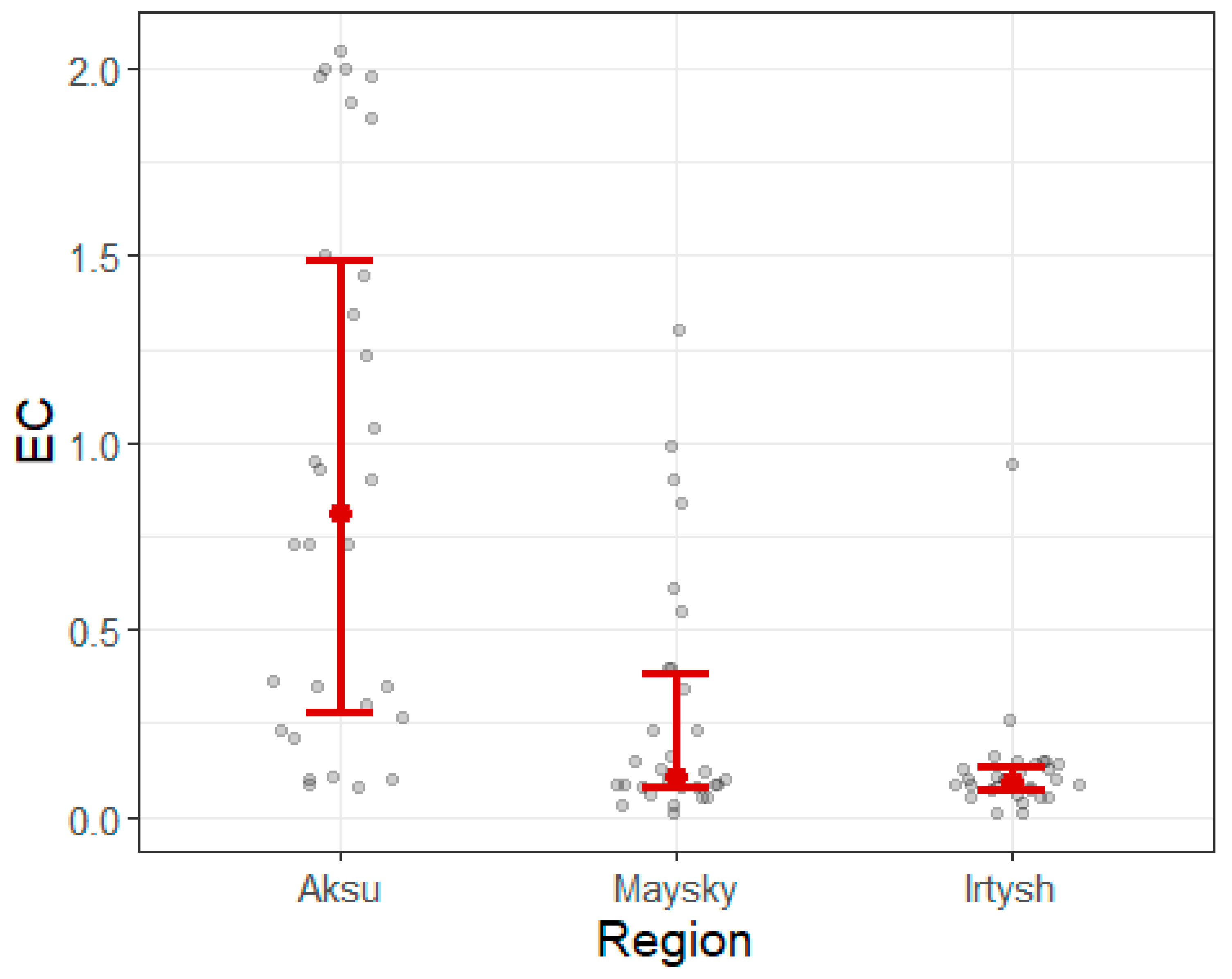
The divergent response of soil salinity to long-term irrigation across the studied districts is a central finding. While irrigation generally led to lower EC values in the Irtysh and Maysky districts compared to their non-irrigated counterparts (indicating a net leaching effect, as shown in Figure 7A and presented in Section 3.1), a secondary salinization (EC > 2 dS/m, ESP > 15%) was observed in the irrigated Haplic Kastanozems of the Aksu district. We hypothesize that these contrasting outcomes are driven by a complex interplay of regional agro-climatic conditions, inherent soil properties, local hydrogeological settings, and potentially differences in historical irrigation management.
In the Irtysh district, dominated by Haplic Chernozems and a more humid climate with higher annual precipitation (287.1 mm, Section 3.2), irrigation likely enhanced natural leaching processes. The regular water supply under irrigation, combined with the potentially deeper groundwater levels and better natural drainage typical for Chernozemic landscapes in less arid conditions, would facilitate effective removal of salts from the root zone, leading to the observed lower EC values on irrigated plots.
In the Maysky district, despite its generally drier conditions compared to Irtysh and the presence of light chestnut soils (Haplic Kastanozems), irrigated plots also exhibited lower EC than non-irrigated ones. This suggests that on the studied sites, irrigation water application was managed in a way that promoted leaching or that the initial salinity of soils and groundwater was not critically high. The data also indicated that precipitation during the hot pre-vegetation period was higher in Maysky than in Aksu (Section 3.2), which might have contributed to a more favorable initial salt balance before the peak irrigation season. It is also possible that groundwater levels in the specific Maysky study plots were deeper or less saline than those encountered in Aksu.
Conversely, the pronounced degradation in the Aksu district (irrigated Haplic Kastanozems) points towards secondary salinization processes intensified by irrigation. This outcome is attributed to a synergistic combination of local agro-climatic, soil, and hydrogeological factors, exacerbated by irrigation inputs. In Aksu, these combined factors appear to have created a scenario where capillary rise and salt accumulation from shallow groundwater overwhelmed any leaching effects of irrigation.
The study design, involving paired comparisons of irrigated and non-irrigated plots on dominant soil types within each distinct agro-climatic district, was chosen to assess the specific impact of irrigation under these varied local conditions. The contrasting results obtained are therefore considered a significant finding, highlighting the site-specific nature of salinization processes and cautioning against generalizing the effects of irrigation without considering the local environmental context.
This pronounced degradation in Aksu, particularly evident when compared to other sites, can be attributed to a synergistic interplay of several local factors:
  • Climate: The Aksu district experiences higher temperatures and lower precipitation compared to Irtysh, leading to significantly higher potential evapotranspiration rates. Irrigation adds the necessary moisture, which then evaporates intensely from the soil surface, concentrating salts and sodium previously present in the soil solution or brought up via capillary rise [2,20];
  • Irrigation and Groundwater Dynamics: Intensive irrigation, likely via center pivots in this area, can easily lead to the rise of already shallow groundwater tables, especially if natural or artificial drainage is suboptimal. Indeed, historical surveys indicate that groundwater depths in the Aksu (formerly Yermak) district often do not exceed 1.8 m [19]. Irrigation likely further elevates these shallow levels, bringing potentially saline groundwater (which may originate from regional saline parent materials, as previously noted) closer to the surface and feeding the evaporative concentration process [40,41];
  • Soil Properties: Chestnut soils (Kastanozems), particularly the sodic variants common in the area, might be inherently more susceptible to structural degradation under irrigation compared to Chernozems. Dispersion of clay particles due to sodium can impede water infiltration and internal drainage, further exacerbating waterlogging and surface salinization [23];
  • Local Site Conditions (Hypothetical): While not measured in this study, specific local factors on the sampled irrigated plot could also play a role. These might include suboptimal local drainage conditions, a longer history of intensive irrigation, or potentially higher salinity in the irrigation water used at this specific site compared to others [19,40].
The soil degradation identified mainly in the irrigated Aksu district, characterized by high EC and ESP values in the topsoil, necessitates the implementation of effective mitigation and management strategies. Based on established practices for saline soil reclamation and prevention of secondary salinization, several approaches appear relevant for the Pavlodar region. Optimizing irrigation water management is paramount. As highlighted by Karimzadeh et al. [35], adopting water-efficient techniques like drip or improved furrow irrigation can minimize excessive water application, reducing deep percolation and the potential for water table rise—a likely contributor to the problems observed in Aksu. Complementary to efficient irrigation is the need for adequate field drainage to control water table depth and facilitate the removal of excess salts. While preventive leaching during the off-season can also aid in salt balance [42], its effectiveness is contingent upon sufficient water availability and functional drainage. Given the sodicity indicated by high ESP in Aksu topsoils, chemical amelioration using calcium-containing amendments like gypsum might be considered to improve soil structure by replacing excess exchangeable sodium [43], although the low SAR values suggest the soil solution itself may not be the primary driver of sodicity at present. Additionally, selecting salt- and sodicity-tolerant crops provides a crucial adaptive strategy for maintaining productivity in affected areas. Ultimately, a sustainable solution requires an integrated approach combining improved engineering (irrigation and drainage) with appropriate agronomic practices and informed decision making by land users.
The critical role of groundwater dynamics in soil salinization, particularly in arid and semi-arid regions like Kazakhstan, is well established. According to a study by Issanova et al. [44], salinization is indeed more common in these arid regions. A primary mechanism involves the accumulation of salinity as groundwater rises towards the earth’s surface due to evaporation; this process is exacerbated if the groundwater outflow rate is less than recharge, leading to a rising water table [45]. While this study did not include direct measurements of groundwater depth and quality, which constitutes a limitation, the observed patterns of salt accumulation, particularly the pronounced surface salinization in the irrigated chestnut soils of the Aksu district, strongly suggest the significant role of shallow groundwater dynamics in the region. High evaporation rates, characteristic of the local climate, likely promote capillary rise from the water table, transporting dissolved salts to the upper soil layer, especially when irrigation practices lead to elevated groundwater levels. The potential severity of this issue, should the groundwater indeed be shallow and saline, is highlighted by existing research. It is known that saline groundwater exacerbates soil salinity, reducing agricultural productivity [46]. Furthermore, studies confirm that salinity risk can often result from highly saline groundwater, particularly when combined with a lack of drainage and associated salinity or alkalinity problems [41]. Specifically, when extremely saline groundwater remains close to the root zone for extended periods without effective drainage, salt accumulation can severely damage root development and lead to significant reductions in crop production [46]. The known prevalence of saline parent materials in parts of the Pavlodar region further underscores the potential risk of elevated groundwater salinity contributing to the observed soil conditions in the study area [19]. Therefore, understanding the local groundwater regime (depth, seasonal fluctuations, and salinity) appears crucial for developing effective strategies to prevent and mitigate secondary salinization in the Pavlodar region. Knowledge of groundwater conditions is essential for selecting appropriate irrigation methods (e.g., favoring drip irrigation where water tables are high to minimize deep percolation and rise) and designing adequate drainage systems. Further research explicitly incorporating groundwater monitoring is highly recommended to confirm the role of groundwater dynamics and salinity and to refine site-specific management recommendations for sustainable agriculture in the region.
The lack of systematic surveys and scientific publications on water resources in the Pavlodar region pose serious challenges to the region’s agricultural sector. Farmers often lack access to up-to-date data on the state of water resources, making it difficult to plan and make informed decisions on farming. Without accurate information, it is impossible to develop effective recommendations on water use, which is especially important in the context of a changing climate and the risk of drought.

5. Conclusions

This investigation highlights that current irrigation practices on chestnut soils within the specific hydro-climatic context of the Aksu district in the Pavlodar region are inducing secondary salinization. This is evidenced by the formation of saline topsoil (0–20 cm) conditions, with electrical conductivity (EC) values typically exceeding 2 dS/m (e.g., averaging 1.54 dS/m) and exchangeable sodium percentage (ESP) values often surpassing 15% (e.g., ranging from 18.04 to 23.63) on irrigated plots. The degradation appears driven by a complex interplay, primarily the interaction between irrigation water inputs, high regional evapotranspiration rates characteristic of Aksu, and the likely influence of historically shallow, potentially saline groundwater dynamics exacerbated by current water management. The inherent properties of the local chestnut soils may further increase their vulnerability to these processes compared to Chernozems in more humid districts, where irrigated soils generally maintained lower salinity levels (e.g., average topsoil EC ~0.11 dS/m).
The findings underscore an urgent need for targeted interventions in the affected areas, particularly Aksu. Sustainable management necessitates a shift towards optimizing water use efficiency, primarily through advanced irrigation techniques (e.g., drip irrigation) to minimize deep percolation, coupled with the implementation or improvement of field drainage systems to effectively control water table depth and facilitate salt leaching. While chemical amelioration and selection of tolerant crops are valuable tools within an integrated strategy, addressing the underlying water management issues appears paramount.
Although this study inferred the role of groundwater due to limitations in direct measurements, the observed salinization patterns (particularly the surface accumulation of salts in irrigated Aksu soils despite relatively low SAR values in soil solution) strongly corroborate existing knowledge regarding the critical influence of shallow groundwater in this arid environment. Therefore, future research and the development of robust, site-specific management strategies for the Pavlodar region critically depend on incorporating systematic monitoring of groundwater levels and quality. This knowledge is essential for fully understanding the hydro-saline processes at play and to design truly sustainable agricultural systems resilient to salinization pressures.

Author Contributions

D.R., writing—review and editing, writing—original draft, visualization, methodology, investigation, formal analysis, data curation, and conceptualization; B.Š., writing—review and editing, writing—original draft, resources, methodology, formal analysis, and conceptualization; M.B., writing—review and editing, visualization, validation, methodology, formal analysis, data curation, and conceptualization; J.Č., validation, methodology, investigation, and formal analysis; K.A., investigation and formal analysis. All authors have read and agreed to the published version of the manuscript.

Funding

This research was funded by Palacký University Olomouc grant, No. IGA_PrF_2025_017.

Institutional Review Board Statement

Not applicable.

Informed Consent Statement

Not applicable.

Data Availability Statement

Data will be made available on request.

Acknowledgments

The authors of the article are grateful for the support of the Palacký University Olomouc grant, No. IGA_PrF_2025_017.

Conflicts of Interest

The authors declare that they have no known competing financial interests or personal relationships that could have appeared to influence the work reported in this paper.

Appendix A. Model Selection Process

This appendix documents the model selection process for each soil property. For each property, we present the systematic model evaluation using a multi-criteria approach including AIC, BIC, Bayes factor, and p-values.

Appendix A.1. Sodium Adsorption Ratio (SAR)

Soilsystems 09 00057 i001
Figure A1. Distribution of Sodium Adsorption Ratio (SAR) values by district (Aksu, Irtysh, Maysky).
Soilsystems 09 00057 g0a1
Soilsystems 09 00057 i002
Figure A2. Sodium Adsorption Ratio (SAR) values by district and irrigation status (irrigated/non-irrigated).
Soilsystems 09 00057 g0a2
Soilsystems 09 00057 i003
Figure A3. Sodium Adsorption Ratio (SAR) values by district and irrigation status, shown for different soil layers.
Soilsystems 09 00057 g0a3

Appendix A.2. pH

Soilsystems 09 00057 i004
Figure A4. Distribution of soil pH values by districts.
Soilsystems 09 00057 g0a4
Soilsystems 09 00057 i005
Figure A5. Soil pH values by districts and soil layers.
Soilsystems 09 00057 g0a5
Soilsystems 09 00057 i006
Figure A6. Soil pH values by district and irrigation status, shown for different soil layers.
Soilsystems 09 00057 g0a6

Appendix A.3. Electrcal Conductivity (EC)

Soilsystems 09 00057 i007
Figure A7. Distribution of Electrical Conductivity (EC) values by districts.
Soilsystems 09 00057 g0a7
Soilsystems 09 00057 i008
Figure A8. Electrical Conductivity (EC) values by districts and irrigation status (irrigated/non-irrigated).
Soilsystems 09 00057 g0a8
Soilsystems 09 00057 i009
Figure A9. Electrical Conductivity (EC) values by districts and irrigation status, shown for different soil layers.
Soilsystems 09 00057 g0a9

Appendix A.4. Exchangeable Sodium Percentage (ESP)

Soilsystems 09 00057 i010
Figure A10. Distribution of Exchangeable Sodium Percentage (ESP) values by districts.
Soilsystems 09 00057 g0a10
Soilsystems 09 00057 i011
Figure A11. Exchangeable Sodium Percentage (ESP) values by districts and irrigation status (irrigated/non-irrigated).
Soilsystems 09 00057 g0a11
Soilsystems 09 00057 i012
Figure A12. Exchangeable Sodium Percentage (ESP) values by district and irrigation status, shown for different soil layers.
Soilsystems 09 00057 g0a12
Conclusion: Full interaction model (RegionFarmHorizons) is clearly superior.

Appendix B

Appendix B.1. Factors Region and Horizons

Appendix B.1.1. ESP

Table A1. Results: Kruskal-Wallis + Dunn test.
TermChi.Squaredp.Value
combo_cat35.550
Residuals
Table A2. Dunn test—ESP.
Irtysh_AIrtysh_BIrtysh_CAksu_AAksu_BAksu_CMaysky_AMaysky_BMaysky_C
1.0001.0001.0001.0001.0001.0000.0200.797
1.000 1.0001.0001.0001.0001.0000.0881.000
1.0001.000 1.0000.3120.8131.0000.4101.000
1.0001.0001.000 1.0001.0001.0000.0040.284
1.0001.0000.3121.000 1.0000.1080.0000.012
1.0001.0000.8131.0001.000 0.3190.0000.044
1.0001.0001.0001.0000.1080.319 1.0001.000
0.0200.0880.4100.0040.0000.0001.000 1.000
0.7971.0001.0000.2840.0120.0441.0001.000

Appendix B.1.2. SAR

Table A3. Results: Kruskal-Wallis + Dunn test.
TermChi.Squaredp.Value
combo_cat34.350
Residuals
Table A4. Dunn test—SAR.
Irtysh_AIrtysh_BIrtysh_CAksu_AAksu_BAksu_CMaysky_AMaysky_BMaysky_C
1.0001.0001.0001.0000.7721.0000.1751.000
1.000 1.0001.0001.0000.8041.0000.1671.000
1.0001.000 1.0000.9450.5221.0000.2741.000
1.0001.0001.000 1.0001.0000.9830.0191.000
1.0001.0000.9451.000 1.0000.0460.0000.069
0.7720.8040.5221.0001.000 0.0200.0000.031
1.0001.0001.0000.9830.0460.020 1.0001.000
0.1750.1670.2740.0190.0000.0001.000 1.000
1.0001.0001.0001.0000.0690.0311.0001.000

Appendix B.1.3. pH

Table A5. ANOVA + Tukey HSD.
DfSum SqMean SqF ValuePr (>F)
20.650.326.010.00
20.630.315.830.00
40.820.213.810.01
814.370.05

Appendix B.1.4. EC

Table A6. Results: Kruskal-Wallis + Dunn test.
TermChi.Squaredp.Value
combo_cat36.670
Residuals
Table A7. Dunn test—EC.
Irtysh_AIrtysh_BIrtysh_CAksu_AAksu_BAksu_CMaysky_AMaysky_BMaysky_C
1.0001.0000.0060.0040.0001.0000.7851.000
1.000 1.0000.0230.0140.0021.0001.0001.000
1.0001.000 1.0000.8340.2141.0001.0001.000
0.0060.0231.000 1.0001.0000.2391.0000.543
0.0040.0140.8341.000 1.0000.1631.0000.386
0.0000.0020.2141.0001.000 0.0310.4820.086
1.0001.0001.0000.2390.1630.031 1.0001.000
0.7851.0001.0001.0001.0000.4821.000 1.000
1.0001.0001.0000.5430.3860.0861.0001.000

Appendix B.2. Factors Region and Farm

Appendix B.2.1. ESP

Table A8. Results: Kruskal-Wallis + Dunn test.
TermChi.Squaredp.Value
combo_cat45.530
Residuals
Table A9. Dunn test—ESP.
Irtysh_IrrigatedIrtysh_Non_irrAksu_IrrigatedAksu_Non_irrMaysky_IrrigatedMaysky_Non_irr
1.0000.0001.0000.2121.000
1.000 0.0091.0000.0220.304
0.0000.009 0.0010.0000.000
1.0001.0000.001 0.1130.997
0.2120.0220.0000.113 1.000
1.0000.3040.0000.9971.000

Appendix B.2.2. SAR

Table A10. Results: Kruskal-Wallis + Dunn test.
TermChi.Squaredp.Value
combo_cat47.740
Residuals
Table A11. Dunn test – SAR.
Irtysh_IrrigatedIrtysh_Non_irrAksu_IrrigatedAksu_Non_irrMaysky_IrrigatedMaysky_Non_irr
1.0000.0001.0000.1651.000
1.000 0.0061.0000.0100.786
0.0000.006 0.0010.0000.000
1.0001.0000.001 0.0501.000
0.1650.0100.0000.050 0.862
1.0000.7860.0001.0000.862

Appendix B.2.3. pH

Table A12. Results: Kruskal-Wallis + Dunn test.
TermChi.Squaredp.Value
combo_cat21.280
Residuals
Table A13. Dunn test—pH.
Irtysh_IrrigatedIrtysh_Non_irrAksu_IrrigatedAksu_Non_irrMaysky_IrrigatedMaysky_Non_irr
0.2200.0021.0001.0001.000
0.220 1.0000.9810.1570.710
0.0021.000 0.0260.0010.015
1.0000.9810.026 1.0001.000
1.0000.1570.0011.000 1.000
1.0000.7100.0151.0001.000

Appendix B.2.4. EC

Table A14. Results: Kruskal-Wallis + Dunn test.
TermChi.Squaredp.Value
combo_cat42.690
Residuals
Table A15. Dunn test – EC.
Irtysh_IrrigatedIrtysh_Non_irrAksu_IrrigatedAksu_Non_irrMaysky_IrrigatedMaysky_Non_irr
1.0000.0000.28311
1.000 0.0000.12811
0.0000.000 0.00900
0.2830.1280.009 11
1.0001.0000.0001.000 1
1.0001.0000.0001.0001

Appendix B.3. Factors Horizons and Farm

Appendix B.3.1. ESP

Table A16. Results: Kruskal-Wallis + Dunn test.
TermChi.Squaredp.Value
combo_cat2.330.8
Residuals
Table A17. Dunn test – ESP.
A_IrrigatedB_IrrigatedC_IrrigatedA_Non_irrB_Non_irrC_Non_irr
11111
1 1111
11 111
111 11
1111 1
11111

Appendix B.3.2. SAR

Table A18. Results: Kruskal-Wallis + Dunn test.
TermChi.Squaredp.Value
combo_cat1.830.87
Residuals
Table A19. Dunn test – SAR.
A_IrrigatedB_IrrigatedC_IrrigatedA_Non_irrB_Non_irrC_Non_irr
11111
1 1111
11 111
111 11
1111 1
11111

Appendix B.3.3. pH

Table A20. Kruskal-Wallis + Dunn test.
TermChi.Squaredp.Value
combo_cat14.490.01
Residuals
Table A21. Dunn test—pH.
A_IrrigatedB_IrrigatedC_IrrigatedA_Non_irrB_Non_irrC_Non_irr
1.0000.1071.0000.8081.000
1.000 0.1091.0000.8191.000
0.1070.109 0.0131.0001.000
1.0001.0000.013 0.1630.262
0.8080.8191.0000.163 1.000
1.0001.0001.0000.2621.000

Appendix B.3.4. EC

Table A22. Kruskal-Wallis + Dunn test.
TermChi.Squaredp.Value
combo_cat9.640.09
Residuals
Table A23. Dunn test—EC.
A_IrrigatedB_IrrigatedC_IrrigatedA_Non_irrB_Non_irrC_Non_irr
1.0001.0000.09911.000
1.000 1.0000.14611.000
1.0001.000 0.12811.000
0.0990.1460.128 10.169
1.0001.0001.0001.000 1.000
1.0001.0001.0000.1691

References

  1. Food and Agriculture Organization of the United Nations (FAO). Guidelines for the Management of Saline Soils; FAO: Rome, Italy, 2017; pp. 3–15. [Google Scholar]
  2. Cirelli, A.; Arumí, J.; Rivera, D. Environmental Effects of Irrigation in Arid and Semi-Arid Regions. Chil. J. Agric. Res. 2009, 69 (Suppl. 1), 27–40. [Google Scholar] [CrossRef]
  3. Huang, Y.; Wang, Y.; Zhao, Y.; Xu, X.; Zhang, J.; Li, C. Spatiotemporal Distribution of Soil Moisture and Salinity in the Taklimakan Desert Highway Shelterbelt. Water 2015, 7, 4343–4361. [Google Scholar] [CrossRef]
  4. Hachicha, M.; Cheverry, C.; Mhiri, A. The Impact of Long-Term Irrigation on Changes of Ground Water Level and Soil Salinity in Northern Tunisia. Arid Soil Res. Rehabil. 2000, 14, 175–182. [Google Scholar] [CrossRef]
  5. Benslama, A.; Khanchoul, K.; Benbrahim, F.; Boubehziz, S.; Chikhi, F.; Navarro- Pedreño, J. Monitoring the Variations of Soil Salinity in a Palm Grove in Southern Algeria. Sustainability 2020, 12, 6117. [Google Scholar] [CrossRef]
  6. Abuelgasim, A.; Ammad, R. Mapping soil salinity in arid and semi-arid regions using Landsat 8 OLI satellite data. Remote Sens. Appl. Soc. Environ. 2019, 13, 415–425. [Google Scholar] [CrossRef]
  7. Telles, T.S.; de Fátima, G.M.; Dechen, S.C.F. The costs of soil erosion [Os custos da erosão do solo]. Rev. Bras. Cienc. Solo. 2011, 35, 287–298. [Google Scholar] [CrossRef]
  8. Šarapatka, B.; Bednář, M. Agricultural Production on Erosion-Affected Land from the Perspective of Remote Sensing. Agronomy 2021, 11, 2216. [Google Scholar] [CrossRef]
  9. Zhao, Y.; Wang, G.; Zhao, M.; Wang, M.; Jiang, M. Direct and indirect effects of soil salinization on soil seed banks in salinizing wetlands in the Songnen Plain, China. Sci. Total Environ. 2022, 819, 152035. [Google Scholar] [CrossRef]
  10. Lech, M.; Fronczyk, J.; Radziemska, M. Monitoring of total dissolved solids on agricultural lands using electrical conductivity measurements. Appl. Ecol. Environ. Res. 2016, 14, 285–295. [Google Scholar] [CrossRef]
  11. Ibraeva, M.A.; Shauharova, D.E.; Dzhumanova, M. Influence of soil salinity on microbiological activity. Pochvovedenie I Agrokhimiya 2020, 2, 71–78. (In Russian) [Google Scholar]
  12. Qadir, M.; Noble, A.; Qureshi, A.; Gupta, R.; Yuldashev, T.; Karimov, A. Salt- induced land and water degradation in the Aral Sea basin: A challenge to sustainable agriculture in Central Asia. Nat. Resour. Forum. 2009, 33, 134–149. [Google Scholar] [CrossRef]
  13. Measho, S.; Li, F.; Pellikka, P.; Tian, C.; Hirwa, H.; Xu, N.; Qiao, Y.; Khasanov, S.; Kulmatov, R.; Chen, G. Soil Salinity Variations and Associated Implications for Agriculture and Land Resources Development Using Remote Sensing Datasets in Central Asia. Remote Sens. 2022, 14, 2501. [Google Scholar] [CrossRef]
  14. United Nations Development Programme (UNDP). Water—Critical Resource for Uzbekistan Future; UNDP: Tashkent, Uzbekistan, 2007; p. 121. [Google Scholar]
  15. Paolo, T.; Jian, L.; Edward, P.; Gianni, B.; Roberta, M. Soil salinization in agriculture: Mitigation and adaptation strategies combining nature-based solutions and bioengineering. iScience 2024, 27, 108830. [Google Scholar] [CrossRef]
  16. Ruto, E.; Tzemi, D.; Gould, I.; Bosworth, G. Economic Impact of Soil Salinization and the Potential for Saline Agriculture. In Future of Sustainable Agriculture in Saline; CRC Press: Boca Raton, FL, USA, 2021; Chapter 6. [Google Scholar] [CrossRef]
  17. Rau, A.; Koibakova, Y.; Balgabayev, N.; Nabiollina, M.; Kurmanbek, Z.; Issakov, Y.; Zhu, K.; David, L.D. Increase in productivity of chestnut soils on irrigated lands of northern and Central Kazakhstan. Land 2023, 12, 672. [Google Scholar] [CrossRef]
  18. Almishev, U.K.; Bondarenko, A.P. Improvement of Meadows and Complex Harvesting: A Tutorial; Toraighyrov University: Pavlodar, Kazakhstan, 2006; pp. 4–46. (In Kazakh) [Google Scholar]
  19. Dzhanpeisov, R.; Sokolov, A.A.; Faizov, K.S. Soils of the Pavlodar Region; Institute of Soil Science: Almaty, Kazakhstan, 1960; pp. 8–13. [Google Scholar]
  20. Baisholanov, S.S. Agroclimatic Resources of Pavlodar Region: Scientific and Applied Reference Book; Institute of Geography: Astana, Kazakhstan, 2017. (In Kazakh) [Google Scholar]
  21. IUSS Working Group WRB. World Reference Base for Soil Resources. International Soil Classification System for Naming Soils and Creating Legends for Soil Maps, 4th ed.; International Union of Soil Sciences (IUSS): Vienna, Austria, 2022. [Google Scholar]
  22. Smailov, S. Peculiarities of regional nature management in Pavlodar region. Bull. Kemerovo State Univ. 2015, 2, 59–64. [Google Scholar]
  23. Rakhmanov, D.; Šarapatka, B.; Alibekova, K.; Černohorský, J.; Hekera, P.; Smanov, Z. Assessment of agricultural land salinization via soil analysis and remote sensing data: Case study in Pavlodar region, Kazakhstan. Soil Water Res. 2024, 19, 111–121. [Google Scholar] [CrossRef]
  24. Lilles, E.B.; Purdy, B.G.; Chang, S.X.; Macdonald, S.E. Soil and groundwater characteristics of saline sites supporting boreal mixedwood forests in northern Alberta. Can. J. Soil Sci. 2010, 90, 1–14. [Google Scholar] [CrossRef]
  25. GOST 26423-85; Soils. Methods for Determination of Specific Electric Conductivity, pH and Solid Residue of Water Extract. Standartinform: Moscow, Russia, 2011.
  26. Zhang, L.; Chang, Y.; Gao, W.; Li, X.; Jiang, H.; Zhou, R.; Ma, X.; Wang, X.; Hai, C.; Xie, Y. Assessment of the Quality Indices of Soils Irrigated by Groundwater in a Typical Semi-Arid Steppe Ecoregion. Pol. J. Environ. Stud. 2022, 31, 1951–1961. [Google Scholar] [CrossRef]
  27. Kaya, F.; Schillaci, C.; Keshavarzi, A.; Başayiğit, L. Predictive Mapping of Electrical Conductivity and Assessment of Soil Salinity in a Western Türkiye Alluvial Plain. Land 2022, 11, 2148. [Google Scholar] [CrossRef]
  28. Drovovozova, T.I.; Panenko, N.N. The study of water extract chemical composition and assessment of salinity degree of irrigated soils adjacent to water collectors of Semikarakorsk district Rostov region. Ecol. Water Manag. 2020, 2, 36–48. [Google Scholar] [CrossRef]
  29. Seilsepour, M.; Rashidi, M.; Khabbaz, B.G. Prediction of soil exchangeable sodium percentage based on soil sodium adsorption ratio. Am.-Eurasian J. Agric. Environ. Sci. 2009, 5, 1–4. [Google Scholar]
  30. Eldiabani, G.S.; Elsbia, S.M. Influence of the temperature on soil’s exchangeable cations and cation exchange capacity, Derna district, Libya: A field and Laboratory study. World J. Adv. Eng. Technol. Sci. 2022, 07, 130–142. [Google Scholar] [CrossRef]
  31. Cumming, G. The New Statistics: Why and How. Psychol. Sci. 2014, 25, 7–29. [Google Scholar] [CrossRef]
  32. Ellison, M. Bayesian inference in ecology. Ecol. Lett. 2004, 7, 509–520. [Google Scholar] [CrossRef]
  33. Lark, R.M.; Cullis, B.R. Model-based analysis using REML for inference from systematically sampled data on soil. Eur. J. Soil Sci. 2004, 55, 799–813. [Google Scholar] [CrossRef]
  34. Burnham, K.P.; Anderson, D.R. Model Selection and Multimodel Inference: A Practical Information-Theoretic Approach, 2nd ed.; Springer: New York, NY, USA, 2002. [Google Scholar]
  35. Karimzadeh, S.; Hartman, S.; Chiarelli, D.; Cristina, R.M.; D’Odorico, P. The tradeoff between water savings and salinization prevention in dryland irrigation. Adv. Water Resour. 2024, 183, 104604. [Google Scholar] [CrossRef]
  36. Solangi, G.S.; Siyal, A.A.; Babar, M.M.; Siyal, P. Spatial Analysis of Soil Salinity in the Indus River Delta, Pakistan. Eng. Technol. Appl. Sci. Res. 2019, 9, 4271–4275. [Google Scholar] [CrossRef]
  37. Dossova, M.; Saparov, K.; Atasov, E. Agricultural influence on landscapes and environmental stability of Pavlodarsky first Republic of Kazakhstan. J. Int. Soc. Res. 2018, 11, 307–310. [Google Scholar] [CrossRef]
  38. Khamidov, M.; Ishchanov, J.; Hamidov, A.; Donmez, C.; Djumaboev, K. Assessment of Soil Salinity Changes under the Climate Change in the Khorezm Region, Uzbekistan. Int. J. Environ. Res. Public Health. 2022, 19, 8794. [Google Scholar] [CrossRef]
  39. Kotuby-Amacher, J.; Koenig, R.; Kitchen, B. Salinity and Plant Tolerance; Utah State University Extension: Logan, UT, USA, 2000; Paper 43; Available online: https://digitalcommons.usu.edu/extension_histall/43 (accessed on 5 February 2025).
  40. Mao, D.; Riesbeck, F.; Khodabakhshi, H.; Mahjoobi, A. The impacts of irrigation and groundwater drainage induced salinity and overflooding of evaporation ponds in Khuzestan, Iran. Front. Water 2025, 7, 1266089. [Google Scholar] [CrossRef]
  41. Kaman, H.; Cetin, M.; Kirda, C. Spatial and temporal evaluation of depth and salinity of the groundwater in large irrigated area in Southern Turkey. Pak. J. Agric. Sci. 2016, 53, 503–510. [Google Scholar] [CrossRef]
  42. Kurishbayev, A.; Kaldybayev, S.; Naushabayev, A.; Mansurova, K. Saline and swampy (waterlogged) soils of Kazakhstan and ways to improve them. Res. Results 2024, 1, 101. [Google Scholar] [CrossRef]
  43. Hranovska, L.; Morozov, O.; Pisarenko, P.; Vozhegov, S. Ecological problems of irrigated soils in the south of Ukraine. Visn. Kharkiv. Natl. Univ. Ser. Geol. Geogr. Ekol. 2022, 57, 282–295. [Google Scholar] [CrossRef]
  44. Issanova, G.T.; Abuduwaili, J.; Mamutov, Z.U.; Kaldybayev, A.A.; Saparov, G.A.; Bazarbaeva, T.A. Saline soils and identification of salt accumulation provinces in Kazakhstan. Arid Ecosyst. 2017, 7, 243–250. [Google Scholar] [CrossRef]
  45. Tessema, N.; Yadeta, D.; Kebede, A.; Ayele, G.T. Soil and Irrigation Water Salinity, and Its Consequences for Agriculture in Ethiopia: A Systematic Review. Agriculture 2022, 13, 109. [Google Scholar] [CrossRef]
  46. Lamsal, K.; Paudyal, G.N.; Saeed, M. Model for assessing impact of salinity on soil water availability and crop yield. Agric. Water Manag. 1999, 41, 57–70. [Google Scholar] [CrossRef]
Figure 1. Study area.
Soilsystems 09 00057 g001
Figure 2. Typical pastureland for Pavlodar region.
Soilsystems 09 00057 g002
Figure 3. Manual soil sampling (a) from irrigated fields and (b) from non-irrigated fields.
Soilsystems 09 00057 g003
Figure 4. Modeling of laboratory data of exchangeable sodium percentage (ESP). Letters (e.g., a, b, bc) above data points in sub-figures (AC) indicate statistically significant differences (p < 0.05) between the compared groups based on post-hoc tests (Kruskal-Wallis + Dunn test, as detailed in Appendix B); groups not sharing a common letter are significantly different. (For detailed statistical results, see Appendix B). (A) Comparison of modeled ESP between districts (Aksu, Irtysh, and Maysky) under irrigated vs. non-irrigated conditions (statistical details: Appendix B.2.1); (B) Comparison of modeled ESP between soil layers (I: 0–20 cm, II: 21–50 cm, and III: 51–100 cm) under irrigated vs. non-irrigated conditions (statistical details: Appendix B.3.1); (C) Comparison of modeled ESP between districts across the three soil layers (I, II, and III) (statistical details: Appendix B.1.1).
Soilsystems 09 00057 g004
Figure 5. Modeling of laboratory data of sodium adsorption ratio (SAR). Letters (e.g., a, b, abcd) above data points in sub-figures (AC) indicate statis-tically significant differences (p < 0.05) between the compared groups based on post-hoc tests (Kruskal-Wallis + Dunn test, as detailed in Appendix B); groups not sharing a common letter are significantly different. (For detailed statistical results, see Appendix B). (A) Comparison of modeled SAR between districts (Aksu, Irtysh, and Maysky) under irrigated vs. non-irrigated conditions (statistical details: Appendix B.2.2); (B) Comparison of modeled SAR between soil layers (I: 0–20 cm, II: 21–50 cm, and III: 51–100 cm) under irrigated vs. non-irrigated conditions (statistical details: Appendix B.3.2); (C) Comparison of modeled SAR between districts across the three soil layers (I, II, and III) (statistical details: Appendix B.1.2).
Soilsystems 09 00057 g005
Figure 6. Modeling of laboratory data of soil pH. Letters (e.g., a, b, ab) above data points in sub-figures (AC) indicate statisti-cally significant differences (p < 0.05) between the compared groups based on post-hoc tests (Kruskal-Wallis + Dunn test and ANOVA + Tukey HSD, as detailed in Appendix B); groups not sharing a common letter are significantly different. (For detailed statistical results, see Appendix B). (A) Comparison of modeled pH between districts (Aksu, Irtysh, and Maysky) under irrigated vs. non-irrigated conditions (statistical details: Appendix B.2.3); (B) Comparison of modeled pH between soil layers (I: 0–20 cm, II: 21–50 cm, and III: 51–100 cm) under irrigated vs. non-irrigated conditions (statistical details: Appendix B.3.3); (C) Comparison of modeled pH between districts across the three soil layers (I, II, and III) (statistical details: Appendix B.1.3).
Soilsystems 09 00057 g006
Figure 7. Modeling of laboratory data of electrical conductivity (EC). Letters (e.g., a, b, abc) above data points in sub-figures (AC) indicate statisti-cally significant differences (p < 0.05) between the compared groups based on post-hoc tests (Kruskal-Wallis + Dunn test, as detailed in Appendix B); groups not sharing a common letter are significantly different. (For detailed statistical results, see Appendix B). (A) Comparison of modeled EC between districts (Aksu, Irtysh, and Maysky) under irrigated vs. non-irrigated conditions (statistical details: Appendix B.2.4); (B) Comparison of modeled EC between soil layers (I: 0–20 cm, II: 21–50 cm, and III: 51- 100 cm) under irrigated vs. non-irrigated conditions (statistical details: Appendix B.3.4); (C) Comparison of modeled EC between districts across the three soil layers (I, II, and III) (statistical details: Appendix B.1.4).
Soilsystems 09 00057 g007
Figure 8. Meteorological data of the study areas during the 2023 growing season of spring crops: (A) average air temperature, °C; (B) precipitation, mm.
Soilsystems 09 00057 g008
Table 1. Statistical characteristics of soil salinity parameters (aggregated across the 0–100 cm soil profile) for irrigated lands and lands without irrigation in different regions, where 1—Irtysh, 2—Aksu, and 3—Maysky.
DistrictsMax.Min.Std. Dev.Average
IrrigatedNon-Irr.IrrigatedNon-Irr.IrrigatedNon-Irr.IrrigatedNon-Irr.
ESP110.38.011.762.382.501.704.925.51
ESP223.638.447.680.45.722.4214.525.004
ESP34.3211.161.240.390.963.372.693.91
SAR10.670.550.120.230.150.100.350.40
SAR22.110.720.70.020.550.201.260.38
SAR30.30.880.10.050.050.280.190.33
pH17.67.816.457.10.320.177.197.4
pH28.17.77.167.140.310.177.67.13
pH37.737.57.067.050.200.157.267.28
EC
ds/cm
10.260.940.040,010.050.220.110.14
EC
ds/cm
22.050.730.90.080.450.231.540.31
EC
ds/cm
30.551.30.050.010.160.430.190.33
Disclaimer/Publisher’s Note: The statements, opinions and data contained in all publications are solely those of the individual author(s) and contributor(s) and not of MDPI and/or the editor(s). MDPI and/or the editor(s) disclaim responsibility for any injury to people or property resulting from any ideas, methods, instructions or products referred to in the content.

