Spatiotemporal Modeling of Soil Water Dynamics for Site-Specific Variable Rate Irrigation in Maize

Abstract

This study aimed to simulate dynamic irrigation management zones (MZs) in two maize fields for a variable rate hose reel fertigation machine (VRFM) with a four-section boom control. Soil moisture content was measured from nine and four soil moisture sensors in Field 1 (8.2 ha) and Field 2 (2.5 ha), respectively, on different dates during the 2022 crop season. Three and five MZs scenarios were simulated per irrigation and the theoretical maps were processed for implementation. The application maps fitted to the VRFM showed significant spatiotemporal variations in irrigation requirements. For instance, in Field 1, 3-MZ modelling showed that the areas requiring high (H), medium (M), and low (L)-level irrigation on 21 July were 1.60, 4.84, and 1.85 ha, respectively, even though the farmer applied uniform rate over the whole field. H-level sub-areas ranged between 1.22 ha (25 July) and 3.25 ha (7 July), showing a coefficient of variation (CV) of 43.32% for the three MZs, whereas H-level sub-areas for the five MZs varied from 0.41 ha (2 July) to 1.49 ha (7 July) with a CV value of 48.84%. High levels of within-field variability can be addressed using precise and dynamic irrigation MZs fitted to the irrigation technology used.

1. Introduction

Water shortages due to climate change are becoming more common and significantly affect agricultural production [1]. Commonly used in arid farming regions and during times of low rainfall, irrigation is the process of adding water to the soil to increase crop growth and replant degraded soil [2]. Irrigation depends on regional climatic conditions; however, as climate change begins to affect new regions that were not affected by drought in the past, the need for irrigation also arises in these regions. According to research and current practices, farmers’ use of irrigation is increasing, even in northern EU countries. In countries where irrigation is widely used, irrigation technologies have improved substantially. Consequently, it is reasonable to assume that irrigation will receive greater attention in parts of the world where it was not a priority before. Precision irrigation is necessary because of the rising demand for water to combat climate concerns. To achieve higher agricultural yields and water savings, it is crucial to choose when and how much to irrigate. The four most popular methods of operation for irrigation scheduling, namely evapotranspiration and water balance (ET-WB), soil moisture status, plant water status, and crop models, along with their advantages and disadvantages, are introduced and contrasted to better understand their fundamental processes and principles [3]. It is necessary to have knowledge of soil properties, including texture, water-holding capacity (WHC), wetness, and crop water requirements, at different growth stages [4].

With the advancement of contemporary sensors and sensing technology, a variety of technologies, such as wireless sensor networks (WSNs), remote sensing (RS), global navigation satellite system (GNSS), geographic information systems (GIS), LoRaWAN, and Bluetooth can now be used to collect field data for precision irrigation. WSNs have been widely used in agriculture for automated irrigation management because they are cost-effective and have low energy consumption [5,6,7,8]. In addition to wired solutions, wireless sensor technologies have become more important and widely used [9], particularly in weather forecasting, early warning systems, soil and crop monitoring, and automated and smart irrigation [10,11,12]. Wireless sensor networks with cloud capabilities are promising because the end-user does not have to handle collecting and storing the data.

It has been well documented that parameters affecting the yield of any crop exhibit spatial and temporal variations [13,14,15,16]. Despite awareness of this, the great majority of farmers today are known to apply a constant rate over the field while they vary the total amount of water from one irrigation to another during the irrigation season depending on the soil, plant, and weather conditions. At present, a limited number of farmers seem to determine irrigation needs based on climate data and some sensor data, if any. One of the most important factors affecting the adoption of precision or smart irrigation technologies is that the accuracy of the moisture sensor changes with time in the field, necessitating occasional calibration. Other factors that cause difficulties for the average end-user include cost, installation, data collection, and interpretation issues. Although the advantages of variable rate irrigation have been documented, the adoption rate of this technology has been low; however, efforts to develop the technology should continue for several reasons, including climate change, declining water resources, nutrient management regulations, and water management policies [17].

The development of variable-rate irrigation control systems has attracted considerable attention since the early 2000s. Some of these studies focused on center-pivot and linearly moving irrigation systems [18,19,20]. The development of smart irrigation systems is of the utmost interest and requires the accurate determination of all parameters affecting irrigation [10,21]. Smart systems require not only sensor-based monitoring but also the integration of Internet of Things (IoT) and cloud technologies [10,22,23,24,25,26]. Ref. [27] reviewed various water management techniques and the use of artificial intelligence (AI) and deep learning (DL), along with the IoT network and case studies. Although previous studies have covered new techniques to apply irrigation water more intelligently, there is still a need to improve the current applications by considering the dynamic variations in irrigation needs within fields more precisely. There have been studies focusing on variable rate irrigation (VRI) using hose reel machines, but they usually use the full-swath width as the lateral resolution [28,29,30,31,32]. There appears to be a research gap regarding improvements in the lateral and longitudinal resolutions of VRI applications using hose reel machines. Furthermore, spatial and temporal changes during the irrigation period should be addressed in the management of VRI.

The general objective of this study was to simulate spatiotemporal variations in irrigation needs of maize crops based on dynamic irrigation management zones using a wireless soil moisture sensor network and GIS capabilities. This study compared the constant user rates of irrigation water on different irrigation dates with that of the sensor-based simulated variable irrigation rate. It assesses the right time and rate for irrigation, determines the accuracy of user rate applications, and analyses the dynamic irrigation management zones to be applied by VRFM.

2. Materials and Methods

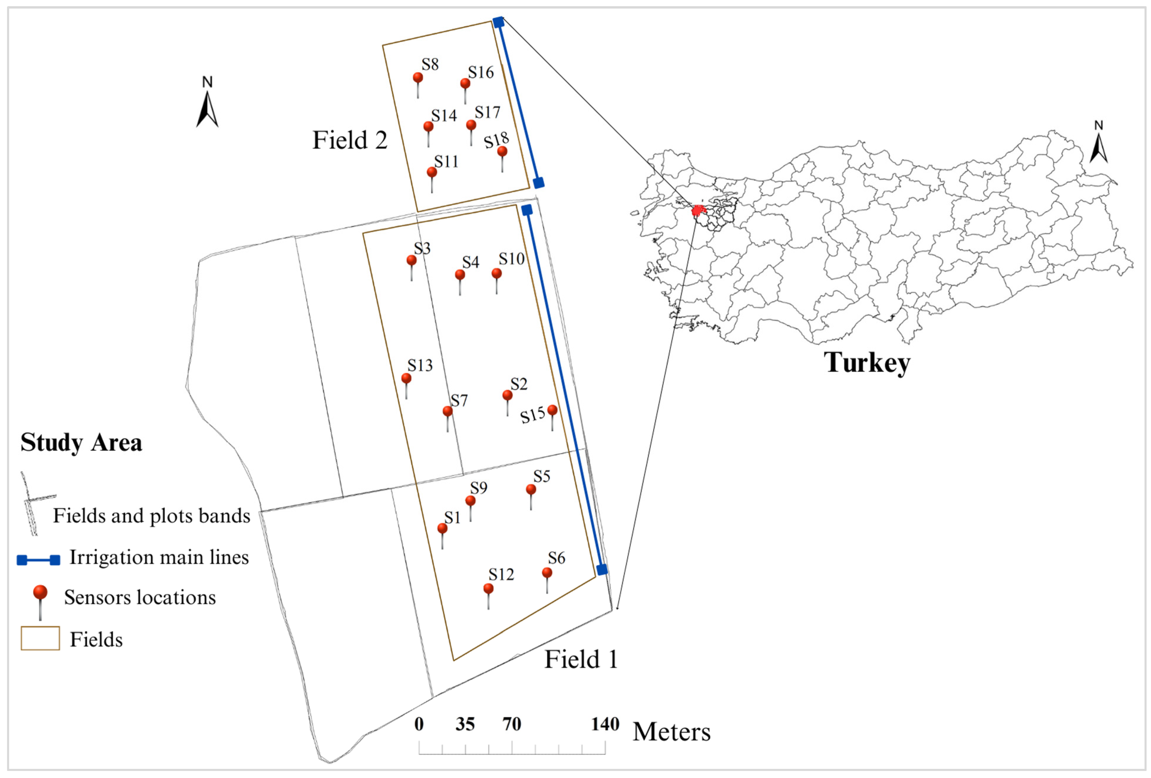
2.1. Site and Irrigation System

The experimental maize fields were located in Bakırköy village of Karacabey, Turkey (40°08′22.61″ N, 28°22′58.7″ E). An 8.2 ha field named Field 1 (F1) and a 2.5 ha field named Field 2 (F2) were selected for the experiment (Figure 1). The soil texture in these fields was composed of 37.6% clay and 32.3% sand in Field 1, and 30.3% clay and 35.3% sand in Field 2. The type of the soil in this study area is alluvial [33]. The fields have approximately rectangular shapes and are irrigated using a closed-loop pressurized wide-area drip irrigation system operated by an irrigation union in the district. The field experiment was conducted during the 2022 growing season. Maize seeds were planted on 16 May 2022 for Field 1 and on 11 May 2022 for Field 2, with the first drip irrigation performed on July 2 for both fields.

The drip irrigation system used during the experiment had drippers delivering 28.8 t h⁻¹ ha⁻¹ irrigation water at an operating pressure of 3 bar. The main and secondary plastic pipes were 200 mm in diameter each. Soil samples were collected randomly at 80 and 30 locations from F1 and F2, respectively, to determine the soil properties (pH, P, K, Mg, Ca, clay, sand, and silt) pertinent to the determination of irrigation needs.

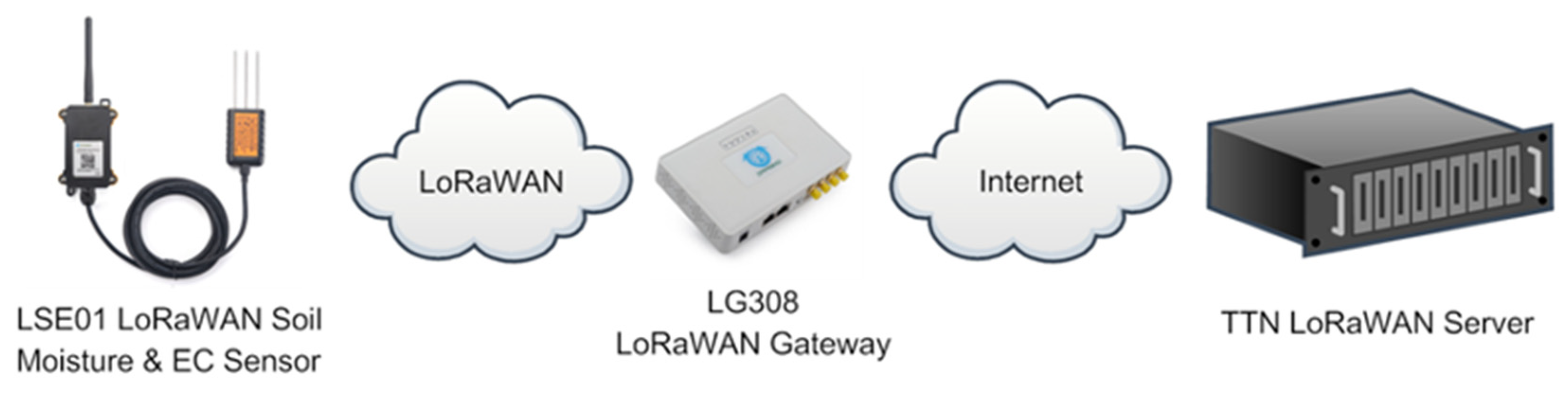
2.2. Wireless Soil Moisture Sensor System

A cloud-based LoRaWAN wireless network was used with soil moisture sensors to collect soil moisture data continuously (Figure 2). Twelve and six MC sensors were installed horizontally at a depth of 300 mm for F1 and F2, respectively. The gateway was approximately 800 m away from the sensors with a clear view of sight. The quantity and placement of the Dragino LSE01 sensors were determined according to the relative management zones (MZs) developed for irrigation. These MZs were delineated based on the precise spatial data on predicted soil MC and clay. The sensors monitored the soil MC ((%) VWC), apparent electrical conductivity (ECa) (uS cm⁻¹), and soil temperature (°C). The sensors enable MC measurements using frequency domain reflectometry (FDR); the accuracy of the MC sensors was reported to be ±3% by the manufacturer.

The accuracy of the sensors was checked during the irrigation season once by collecting soil samples at sensor locations, resulting in approximately 3–5% error in soil moisture measurements. No further investigations were undertaken to check or improve the measurement accuracy of MC sensors.

2.3. Methods

The variable irrigation needs were determined by monitoring the water status using soil moisture content (MC) sensors by previous researchers [35,36] and the same method was used for the experimental fields in this study. Field capacity (FC), permanent wilting point (PWP), and volumetric weight (VW) were determined under laboratory conditions for each soil sample at each sensor location. Undisturbed soil samples were collected. VV was determined by drying soil samples in an oven for 24 h at 105 °C. The sand/kaolin box instrument (Eijkelkamp, Giesbeek, The Netherlands) was used to determine field capacity at 2.54 pF (0.34 bar). The permanent wilting point at a pressure of 4.2 pF (15.20 bar) was determined using a pressure membrane apparatus (Eijkelkamp, Giesbeek, The Netherlands). Available water (AW), management allowable depletion (MAD), and amount of irrigation water (irrigation need, IN) were determined based on laboratory analyses of the soil samples. IN was calculated based on the moisture content (MC) value of the soil to reach the FC values at a given location in the field. The following formulae were used to determine the aforementioned parameters:

$$\mathrm{F}\mathrm{C}\left[\mathrm{m}\mathrm{m}\right]=\mathrm{F}\mathrm{C}\left[\mathrm{\%}\right]\ast \mathrm{V}\mathrm{W}\left[{\mathrm{g}\mathrm{c}\mathrm{m}}^{-3}\right]\ast \mathrm{d}\mathrm{e}\mathrm{p}\mathrm{t}\mathrm{h}/100$$

(1)

$$\mathrm{P}\mathrm{W}\mathrm{P}\left[\mathrm{m}\mathrm{m}\right]=\mathrm{P}\mathrm{W}\mathrm{P}\left[\mathrm{\%}\right]\ast \mathrm{V}\mathrm{W}\left[{\mathrm{g}\mathrm{c}\mathrm{m}}^{-3}\right]\ast \mathrm{d}\mathrm{e}\mathrm{p}\mathrm{t}\mathrm{h}/100$$

(2)

$$\mathrm{A}\mathrm{W}\left[\mathrm{m}\mathrm{m}\right]=\mathrm{F}\mathrm{C}\left[\mathrm{m}\mathrm{m}\right]-\mathrm{P}\mathrm{W}\mathrm{P}\left[\mathrm{m}\mathrm{m}\right]$$

(3)

$$\mathrm{M}\mathrm{A}\mathrm{D}\left[\mathrm{m}\mathrm{m}\right]=\mathrm{P}\mathrm{W}\mathrm{P}+\mathrm{A}\mathrm{W}\left[\mathrm{m}\mathrm{m}\right]\ast \mathrm{M}\mathrm{A}\mathrm{D}\mathrm{s}\mathrm{e}\mathrm{t}\mathrm{t}\mathrm{i}\mathrm{n}\mathrm{g}$$

(4)

$$\mathrm{M}\mathrm{C}\left[\mathrm{m}\mathrm{m}\right]=\mathrm{M}\mathrm{C}\left[\mathrm{\%}\right]\ast \mathrm{V}\mathrm{W}\left[{\mathrm{g}\mathrm{c}\mathrm{m}}^{-3}\right]\ast \mathrm{d}\mathrm{e}\mathrm{p}\mathrm{t}\mathrm{h}/100$$

(5)

$$\mathrm{I}\mathrm{N}\left[\mathrm{m}\mathrm{m}\right]=\left[\mathrm{F}\mathrm{C}\right[\mathrm{m}\mathrm{m}]-\mathrm{M}\mathrm{C}[\mathrm{m}\mathrm{m}\left]\right]/\mathrm{E}\mathrm{F}$$

(6)

where depth is the plant root depth (300 mm in this study). From Equations (1), (2), and (5), the absolute values for FC, PWP, and MC in mm of water column were calculated for the root depth using the relative FC, PWP, and MC in percent and the measured volumetric weight of the soil.

Available water is the difference between FC and PWP (Equation (3)). It represents the range of moisture that is theoretically available for plants, although at moisture levels nearing PWP, plants will start experiencing water stress. To prevent water stress, a management allowable depletion (MAD) is set, which is located between FC and PWP. In Equation (4), MAD setting was considered as 50% of the available water (AW), according to [37].

The irrigation efficiency (EF) was taken (Equation (6)) as 90% for the drip irrigation system [38], to calculate sensor-based irrigation needs based on field capacity and moisture measurement. The irrigation time was based on MAD + 30% limit, which was taken to be 30% of the difference between the FC and MAD values.

The irrigations started before the sensors were ready to collect real-time MC data. After processing the sensor data, only eight irrigation applications were considered for the analyses.

2.3.1. Water Use Comparison between User- and Sensor-Based Constant Irrigation Rates

The farmer used inline linear drippers (Eurodrip-Eolos, Rivulis, Gvat, Israel) in the irrigations with an irrigation intensity of 28.8 t h⁻¹ ha⁻¹ at an operating pressure of 3 bar. The pressure at the end of each secondary line was measured using a handheld analog pressure gauge (Pakkens 0–6 bar) so that the flow rate was the same and the water distribution was uniform in each irrigation plot. For each irrigation, the farmer varied the irrigation time from 6 to 10 h per irrigation, depending on the job and employee status. The user irrigation rate was determined by the experience of the farmer, crop water demands given in the irrigation guide for the Bursa-Karacabey district, and evapotranspiration values provided by the farmer’s weather station (Metos IMT280).

Wireless MC sensors were configured to deliver MC data every 20 min in this study. To confirm a sensor-based constant irrigation recommendation on a given irrigation day, the MC value measured just before irrigation was obtained from each sensor, and the average of all sensor readings was used as the sensor-based field-scale soil MC value. Equation (6) was used to determine the amount of water to be applied (irrigation need) to bring the moisture content of the field to the field capacity for a given irrigation date. The differences among the soil moisture sensor measurements for each irrigation date were calculated to reveal the range of soil moisture content within the field. Within-field soil moisture content variations were evaluated to assess the accuracy of uniform irrigation in the trial fields. A descriptive statistics analysis was performed in terms average, difference, standard deviation, and coefficient of variance (CV).

2.3.2. Variable Rate Irrigation Recommendations

The ordinary kriging (OK) interpolation method was implemented using ArcGIS ArcMap v10.8 (ESRI Redlands, Redlands, CA, USA) software to generate variable rate irrigation (VRI) maps. The irrigation needs (IN, mm da⁻¹, where 1.0 da = 0.1 ha) were mapped with three and five management zones (MZs) for each field to compare the effects of different resolutions for irrigation. The three and five MZs were selected to see the effects of the number of MZs on the variability in irrigation needs.

First, a theoretical application map was produced for the irrigation dates (2, 5, 7, 13, 17, 21, 25 July and 4 August) for F1 and F2, resulting in 32 maps (8 days × 2 different zone maps × 2 fields). The amount of water to be applied in each irrigation MZ was tabulated based on the irrigation rate and the total area of each irrigation management zone in each field. The user-applied uniform rates and variable-rate irrigation recommendations were then compared to meet the irrigation demands of the soil based on the postulated irrigation zones.

Then, the theoretical 3- and 5-zone irrigation need maps were further processed for VRI application to be applied using a variable rate hose reel fertigation system being developed as part of the project. The VRFM has a working width of 46 m, and it is proposed to have four sections, each to be individually controlled for VRI applications. Thus, using theoretical maps, applicable irrigation maps were obtained for cell sizes of 11.5 m × 1 m. Applicable maps were presented for the irrigation dates of 7, 17, and 25 July and 4 August to discuss the effect of management zones on the water distribution within the fields and were compared with theoretical IN maps.

Sentinel 2A satellite data were used to generate the Normalized Difference Vegetation Index (NDVI) maps corresponding to the nearest irrigation dates. The Sentinel-2A images were downloaded from https://scihub.copernicus.eu/dhus/#/home (accessed on 14 September 2023) in bottom-of-atmosphere L2A format. A total of eight images from 1 July, 6 July, 13 July, 21 July, 26 July, and 5 August 2022, covering the study area, atmospherically corrected, and cloudless were used for analysis. For each S2 scene, the red (band 4), and NIR (band 8) spectral bands with a 10 m spatial resolution were selected for the NDVI calculation according to [39] formula.

Additionally, the texture (clay, silt, and sand) was mapped for F1 and F2 in an attempt to find potential cause-and-effects of NDVI and soil texture on the spatiotemporal variations in irrigation water needs across the fields studied.

3. Results and Discussion

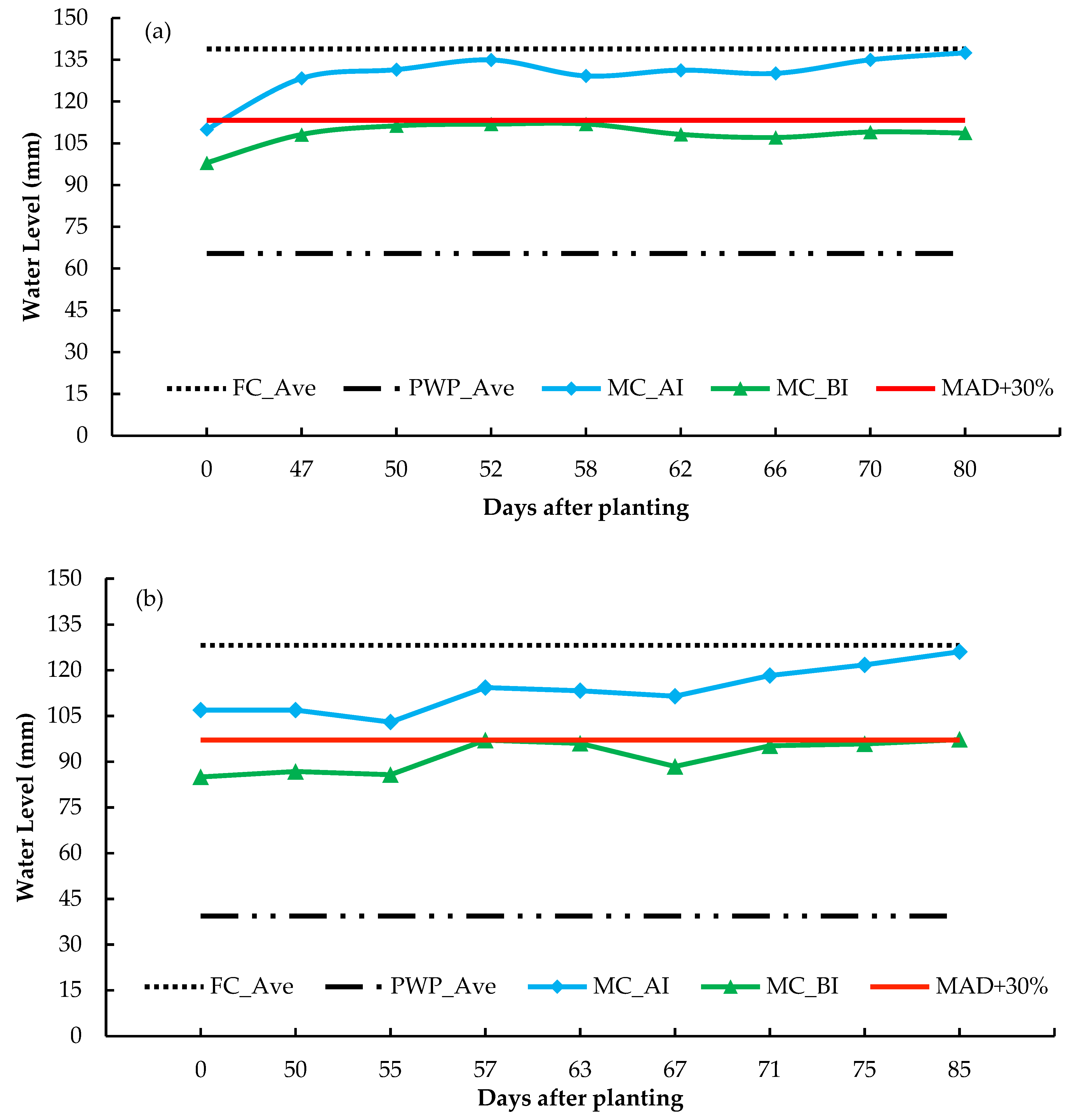
3.1. User-Rate and Sensor-Based Constant Irrigation Comparisons

Nine out of twelve sensors were utilized for soil moisture measurements due to unexpected weak signals, battery, or installation problems in three of the sensors installed in F1; four of the six sensors were operable in F2 (

Table 1. Laboratory results for soil samples taken at the sensor locations for Field 1 and Field 2.

	Sensor No	FC (%)	PWP (%)	VW (g cm−3)	FC (mm)	PWP (mm)	AW (mm)	MAD (mm)
F1	S2	32.49	14.80	1.45	141.10	64.27	76.84	102.69
	S3	29.17	14.38	1.47	128.41	63.28	65.13	95.85
	S5	32.88	15.28	1.42	139.72	64.94	74.78	102.33
	S7	31.66	15.99	1.44	137.10	69.24	67.86	103.17
	S9	32.96	16.36	1.43	141.50	70.25	71.25	105.87
	S10	29.12	12.92	1.50	131.11	58.19	72.92	94.65
	S12	34.03	15.74	1.42	144.51	66.82	77.70	105.66
	S13	32.21	16.09	1.44	139.28	69.56	69.71	104.42
	S15	33.86	15.01	1.45	147.68	65.47	82.21	106.58
	Ave	32.04	15.17	1.45	138.94	65.78	74.16	102.36
	Std	1.80	1.07	0.03	6.07	3.78	5.32	4.30
	CV (%)	5.62	7.03	1.82	4.37	5.75	7.28	4.20
F2	S8	28.07	9.87	1.56	131.58	46.27	85.31	88.92
	S11	28.79	11.10	1.52	130.91	50.47	80.44	90.69
	S14	27.40	6.61	1.56	127.92	30.87	97.05	79.39
	S18	28.00	6.87	1.46	122.38	30.05	92.33	76.22
	Ave	28.06	8.61	1.52	128.20	39.41	88.78	83.81
	Std	0.57	2.22	0.05	4.19	10.49	7.36	7.09
	CV (%)	2.02	25.77	3.18	3.27	26.61	8.29	8.46

F1, field 1; F2, field 2; FC, field capacity; PWP, permanent wilting point; AW, available water; MAD, management-allowable depletion; VW, volumetric weight; Ave, average; Std, standard deviation; CV, coefficient of variation.

). The average FC, PWP, and MAD values in F1 were approximately 139, 66, and 37 mm, respectively. The average volumetric weight of the soil samples was 1.45 (g cm⁻³) with a small coefficient of variation (CV) value (1.82%). Other parameters included in Table 1 had variations with CV values ranging from approximately 4.2 to 7.3%. In F2, based on measurements performed by the four soil moisture sensors, the FC was smaller and VW was higher compared with F1. The MAD values were smaller than those of F1. The coefficient of variation of the measured parameters in F2, except for PWP, ranged from 2.02 to 8.46%. The high CV value of PWP may be attributed to the fewer sensors used, and hence, to fewer data points to be averaged.

The irrigation duration determined by the farmer varied from 7 to 10 h depending on the weather, crop conditions, and labor availability (

Table 2. Irrigation needs to reach field capacity for each irrigation date based on average MC from all sensors for Field 1 and Field 2.

Irrigation Date		MC_BI (mm)	Irrigation Duration (h)	User Rate (mm da−1)	Recommended (mm da−1)	% Difference (mm da−1)
F1	2 July	108.17	7	20.16	30.73	−34.4
	5 July	111.3	7	20.16	27.6	−26.9
	7 July	111.9	8	23.04	27.0	−14.7
	13 July	111.93	6	17.28	26.97	−35.9
	17 July	108.23	8	23.04	30.7	−24.9
	21 July	107.1	8	23.04	31.8	−27.6
	25 July	109.07	9	25.92	29.83	−13.1
	4 August	108.7	10	28.8	30.2	−4.6
	Average	109.55	7.9	22.68	32.65	−22.76
F2	2 July	86.78	7	20.16	46.03	−56.20
	5 July	85.73	6	17.28	47.19	−63.38
	7 July	97.05	6	17.28	34.61	−50.07
	13 July	96.00	6	17.28	35.78	−51.70
	17 July	88.43	8	23.04	44.19	−47.86
	21 July	95.25	8	23.04	36.61	−37.06
	25 July	95.85	9	25.92	35.94	−27.88
	4 August	97.28	10	28.80	34.36	−16.18
	Average	92.79	7.50	21.60	39.34	−45.09

F1, field 1; F2, field 2; MC_BI, moisture content before irrigation.

). More water should have been applied throughout the season to align the soil MC with the FC. For instance, on July 7, the applied user rate was 23.04 t da⁻¹ as a result of 8 h irrigation, which was 14.7% less than the recommended rate based on the average of the soil MC measurements. The overall average of user rates was 22.68 mm da⁻¹ while the sensor-based application rate was calculated to be 29.83 mm da⁻¹. The overall difference between the user and sensor-based rates was −22.76%, whereas the differences ranged from −4.6% to −35.9% on specific dates. This means that the soil received a smaller amount of water than it should have if the moisture sensor data would have been used to calculate the irrigation rate. It can be concluded that the irrigation duration could be adjusted more accurately by the farmer if moisture sensor data were used to align the available MC with the FC level.

In F2, the ranges of irrigation rates for the user- and sensor-based irrigations were 17.28–28.80 mm da⁻¹ and 27.0–47.19 mm da⁻¹, respectively (Table 2). On average, throughout the irrigation season, the user-based rate of irrigation water application was 45.09% less than the recommended IN. In this case, the difference was more significant than that for F1. Although the farmer intended to apply water every 3–4 days after 7 July, due to labor shortage, an irrigation was skipped between 7 July and 13 July. Automated irrigation systems can reduce the dependency on workers to accomplish time-dependent tasks.

It should be noted that the above discussion does not account for spatial variations in irrigation needs within a field. Even for a constant irrigation rate at the whole-field scale, the use of soil moisture sensors revealed opportunities for implementing irrigation at more accurate times and rates. In [40], it was concluded that the total profit was the same when sensor-based irrigation scheduling was compared with the user application, but the sensor-based application was found to be promising in terms of water and financial savings.

The variations in the measured MC values on specific irrigation dates are shown in Figure 3 for F1 and F2. Figure 3 also presents the average FC, PWP, and MAD values to visualize when irrigation had to be started and terminated.

The MC values were expected to be around the MAD line before the irrigation started and near the FC line after the irrigation was completed. The farmer always started irrigation at a soil moisture content slightly below the MAD + 30% value in F1 (Figure 3a). The irrigation timings were slightly after than the exact irrigation times. After irrigation, the soil MC was always lower than the FC. The farmer applied irrigation water that did not exceed the FC for the entire field. However, the timing and duration of the user rate can be improved by using the average soil moisture readings made by the sensors so that the soil MC values reach FC.

At the early growth stages of maize plants, the penetration of the maize roots is shallower than in the later stages [3]; thus, maintaining the topsoil moisture should be more important to avoid water stress. The soil tended to generate cracks owing to the lack of moisture, especially during windy periods that are common in the region. Therefore, it may be recommended to start irrigation earlier than occurred because the measured MC values before irrigation were lower than the MAD + 30% values. MC values below the MAD + 30% value in Figure 3a,b suggest that plants might have experienced water stress during the early growth stages. To prevent this, frequent and sufficient irrigation could have been determined using the sensor-based data.

Figure 3b suggests that the timing of irrigation was not accurate for some irrigation dates in Field 2. The farmer started irrigating the field at a soil MC level lower than the MAD + 30% value in four of the irrigations. Furthermore, irrigation was terminated too early since the after-irrigation soil MC values were just above the MAD + 30% values and not reaching the targeted FC values. As demonstrated in Figure 3b, real-time data could be used to accurately determine the correct length and amount of irrigation, either done manually or automatically.

FC and after-irrigation MC values were compared on each irrigation day (

Table 3. Percent user difference between after-irrigation moisture content and field capacity (FC) for Field 1 and Field 2.

F1						F2
Irrigation Date	FC_Ave (mm)	MC_BI (mm)	MC_AI (mm)	Diff. (mm)	%User Diff.	FC_Ave (mm)	MC_BI (mm)	MC_AI (mm)	Diff. (mm)	%User Diff.
2 July	138.9	108.2	128.3	10.6	−7.6	128	87	107	21	−17
5 July	138.9	111.3	131.5	7.5	−5.4	128	86	106	22	−17
7 July	138.9	111.9	134.9	4	−2.9	128	97	120	8.1	−6.3
13 July	138.9	111.9	129.2	9.7	−7	128	96	113	15	−12
17 July	138.9	108.2	131.3	7.7	−5.5	128	88	112	17	−13
21 July	138.9	107.1	130.1	8.8	−6.3	128	95	118	9.9	−7.7
25 July	138.9	109.1	135	4	−2.8	128	96	122	6.4	−5
4 August	138.9	108.7	137.5	1.4	−1	128	97	126	2.1	−1.7

F1, field 1; F2, field 2; FC_Ave, average field capacity; MC_BI, before-irrigation moisture content; MC_AI, after-irrigation moisture content; Diff., absolute difference between the soil moisture content and the field capacity; %diff., difference between MC_AI and FC.

). The MC of the soil was approximately 110 mm before irrigation and increased to 128.2–137.5 mm while the average FC was 138.9 mm for the field. The percent user difference in irrigation needs between the user and the average sensor readings varied from 1% to 7.6%, implying that the user should have applied slightly more water to bring the MC values to the FC level at the field scale.

Table 3 shows the user applications compared with the after-irrigation MC-based measurements for F1 and F2. The user started irrigation when the soil MC value was between 86 mm and 97 mm in the field, depending on the irrigation date. The MC values following irrigations were between 107 and 126 mm. The applied water was less than the amount of water necessary to increase the soil MC values up to an average FC level of 128 mm in Field 2. Up to 17% more water should have been applied in Field 2 on 2 and 5 July, corresponding to the early growth stages of plants.

The spatial variation in the before-irrigation MC values for each irrigation day is shown in

Table 4. Average irrigation needs (mm da⁻¹) per irrigation and maximum differences among sensors for Field 1 and Field 2.

	Sensor No.	2 July	5 July	7 July	13 July	17 July	21 July	25 July	4 August
F1	S2	18.12	12.12	10.12	18.12	19.78	19.45	19.45	19.78
	S3	12.68	8.01	8.35	8.68	12.35	15.35	16.01	18.68
	S5	28.25	27.58	27.58	23.58	22.25	25.58	22.25	20.25
	S7	34.00	31.33	31.33	35.33	36.67	30.00	28.67	35.33
	S9	37.22	41.89	41.56	36.22	37.22	37.56	35.22	24.56
	S10	47.34	41.67	41.67	36.34	42.67	45.01	48.01	43.67
	S12	40.24	40.24	40.24	36.57	47.57	52.90	51.90	52.90
	S13	34.75	19.09	15.42	26.09	35.09	40.42	24.09	38.09
	S15	55.09	54.42	54.09	49.09	53.42	52.09	53.09	49.09
	Ave	34.2	30.7	30.0	30.0	34.1	35.4	33.2	33.6
	Std	13.3	15.4	16.0	12.1	13.5	13.6	14.5	13.3
	%CV	39	50	53	40	40	39	44	40
	Max diff (%)	0.77	0.85	0.85	0.82	0.77	0.71	0.70	0.65
F2	S8	39.20	40.20	39.20	36.20	38.20	32.20	26.20	30.86
	S11	43.79	44.12	25.46	36.12	45.79	39.12	37.79	23.79
	S14	53.80	57.13	28.80	36.46	50.13	44.13	45.46	46.46
	S18	47.32	47.32	44.98	34.32	42.65	30.98	34.32	36.32
	Ave	46.03	47.19	34.61	35.78	44.19	36.61	35.94	34.36
	Std	6.2	7.2	9.1	1.0	5.0	6.2	8.0	9.6
	%CV	13.4	15.3	26.2	2.7	11.4	16.8	22.2	27.8
	Max diff (%)	0.27	0.30	0.43	0.06	0.24	0.30	0.42	0.49

F1, field 1; F2, field 2; S, sensor number; Ave, average; Std, standard deviation; CV, coefficient of variation; Max diff, maximum difference.

, where the first column shows the sensors installed in both fields. On average, the IN was between 30 and 35.5 mm before irrigation in F1. However, the IN was calculated to range from 35.94 to 47.19 mm for F2, which was a wider range than for F1.

The average irrigation need for each irrigation date was greater in F2 than in F1, probably because of the different ranges between the FC and PWP, and hence the MAD values in the two fields. The average MAD value of F1 was greater than that of F2, requiring more water delivery to irrigate the field up to field capacity.

3.2. Constant vs. Variable Rate Irrigation

As discussed in the previous subsection, irrigation scheduling based on soil moisture sensors has the potential to improve the timing and amount of irrigation water required. However, the above discussion was based on the average of all readings from the soil moisture sensors. As the sensors were in different parts of the field, it would be more useful to determine the spatial irrigation needs on a given irrigation day.

Table 5. The percent difference between the average sensor readings to point-based moisture content (MC) readings for each irrigation date for Field 1 and Field 2.

	Sensor No.	2 July	5 July	7 July	13 July	17 July	21 July	25 July	4 August
F1	S2	15.4	17.0	18.0	11.5	13.9	15.4	13.3	13.4
	S3	8.2	8.9	8.0	7.7	8.4	7.0	4.5	2.7
	S5	5.7	3.2	2.7	5.9	10.6	9.0	9.7	11.8
	S7	−1.5	−2.2	−2.7	−5.9	−3.8	2.8	2.0	−3.1
	S9	−0.2	−6.7	−7.0	−2.7	−0.2	0.6	0.7	9.8
	S10	−18.2	−15.9	−16.4	−12.1	−14.4	−15.4	−19.4	−15.5
	S12	0.1	−2.7	−3.2	−0.3	−6.0	−9.5	−10.3	−10.9
	S13	−0.2	9.7	12.1	3.5	−0.5	−3.9	7.8	−3.4
	S15	−9.3	−11.3	−11.5	−7.5	−8.0	−5.9	−8.4	−4.8
F2	S8	11.0	11.3	−0.8	3.1	9.9	7.7	12.7	6.7
	S11	5.4	6.4	11.3	2.5	1.4	0.5	1.1	12.6
	S14	−8.4	−10.8	5.1	−0.9	−6.4	−7.4	−9.2	−11.5
	S18	−8.0	−6.9	−15.6	−4.7	−5.0	−0.8	−4.5	−7.8

shows the difference between the average before-irrigation MC values and point-based MC values on each irrigation day. The data show that some parts of the field required more or less water than the previously calculated average IN. For instance, on 13 July, 11.5% more water would have been applied at S2, whereas 12.1% less water would have been applied at S10 if the average before-irrigation MC values had been used. Similarly, in F2, a maximum of 12.7% more and 11.5% less water would have been applied on 25 July at S8 and 4 August at S14, respectively, if the average of all MC sensors had been used to determine the irrigation need.

The spatiotemporal changes in the soil MC values show that the irrigation needs vary within the fields; hence, appropriate precision application technologies should be developed to account for these variations (Figure 4).

The variations in the soil MC in F1 during the monitoring period showed that the upper-left corner of the field always had lower moisture content values and the lower-left corner had the greatest measured MC values. Other parts of the field showed varying degrees of change in the level of water requirements.

Figure 4 and Figure 5 show the three- and five-zone irrigation management zones for F1 and F2. These figures show the same patterns in irrigation needs with different precisions with low (L), medium-low (ML), medium (M), medium-high (MH), and high (H) application rates.

The analysis of five irrigation management zones suggests that irrigation water can be delivered more precisely to areas needing different irrigation rates, for example, M, ML, L, MH, and H levels. However, accurately applying five different application rates based on the management zones is unlikely considering the layout of the current drip irrigation systems in use. Thus, it may be concluded that the maps obtained by the OK method are useful for revealing the spatiotemporal variabilities within the fields but need to be processed for use with the most appropriate irrigation technology available, for example, hose reel or pivot systems with, at minimum, section control mechanisms.

The Irrigation maps for F2 in Figure 5 show that the areas requiring the least amount of water moved from the top-left corner (2 July and 5 July) to the bottom-left (7 July) and bottom-right (13 July) sides of the field.

The locations of the areas needing the least amount of water continued to change for the remaining F2 during the irrigation season. The irrigation simulation maps in Figure 6 and Figure 7 show different behaviors compared to F1, in that the dynamic changes in the spatial IN requirements can be prominent over time.

Table 6. Variation in area (ha) of each management zone over time for variable irrigation based on OK for Field 1 and Field 2.

		3 MZs			5 MZs
	Irrigation Date/Rate	H	M	L	H	MH	M	ML	L
F1	2 July	1.60	5.36	1.32	0.41	1.18	3.06	2.58	1.05
	5 July	0.90	4.26	3.12	0.14	0.75	2.82	1.97	2.60
	7 July	3.26	3.45	1.57	1.44	3.28	2.00	1.11	0.46
	13 July	3.56	3.58	1.14	0.72	4.26	2.17	0.55	0.59
	17 July	1.80	5.53	0.95	0.49	1.31	4.09	1.44	0.95
	21 July	1.54	4.95	1.79	1.20	1.76	3.53	1.11	0.68
	25 July	1.20	3.08	4.00	0.65	1.06	2.08	2.51	1.98
	4 August	1.35	4.93	2.01	0.40	1.20	3.07	2.65	0.97
	Ave.	1.90	4.39	1.99	0.68	1.85	2.85	1.74	1.16
	Std dev.	0.98	0.94	1.06	0.43	1.24	0.74	0.80	0.74
	%CV	51.31	21.28	53.11	63.67	67.24	26.10	45.94	64.21
F2	2 July	0.27	1.69	0.54	0.13	0.38	1.24	0.48	0.28
	5 July	0.52	1.50	0.49	0.29	0.23	0.96	0.53	0.49
	7 July	0.49	1.21	0.80	0.33	0.69	0.69	0.30	0.49
	13 July	0.94	1.01	0.56	0.32	0.93	0.50	0.30	0.46
	17 July	0.11	0.83	1.56	0.11	0.32	0.51	0.99	0.57
	21 July	0.56	0.96	0.99	0.21	0.34	0.30	0.66	0.99
	25 July	0.78	1.43	0.29	0.16	0.62	0.97	0.46	0.29
	4 August	0.22	1.55	0.74	0.13	0.24	1.39	0.47	0.27
	Ave.	0.49	1.27	0.75	0.21	0.47	0.82	0.52	0.48
	Std dev.	0.28	0.31	0.39	0.09	0.25	0.38	0.22	0.23
	%CV	57.97	24.64	52.65	43.69	53.08	46.66	42.57	48.91

L, low; ML, medium-low; M, medium; MH, medium-high; H, high.

shows the partitioning of the sub-section areas of the three- and five-zone irrigation maps for F1 and F2 derived from the maps in Figure 4 and Figure 5, respectively.

The H level irrigation rate corresponded to areas from 0.89 ha to 32.6 ha with five-zone analysis in F1 whereas three-zone analysis resulted in 0.14 ha to 14.3 ha for H level rates on different irrigation days. Dividing the field into management zones shows that different parts of the field require different application rates to bring the soil MC to the FC. Five zones depicted the distribution of the rates more precisely for each irrigation date. In F2, the zone areas were smaller due to the smaller field size compared to that of F1. The CV values from about 45–65% both for F1 and F2 also show that the application rates for each zone need to be changed significantly over time. For instance, the CV level of 46.7% for M level area in the five-zone analysis was found in areas ranging from 3.0 ha (21 July) to 13.87 ha (4 August). The IN maps shown in Figure 5, Figure 6, Figure 7 and Figure 8 are not readily applicable because of the lack of precise application technologies that can deliver irrigation water based on contour maps. The length of the lateral pipes in a drip irrigation system is designed to be the same length in each management zone in sub-plot areas of up to four hectares in the current practices in the Karacabey district, intersecting with the simulated IN maps. Furthermore, the dynamic variation in the irrigation management zone from one irrigation to the next requires an irrigation system that can respond accordingly.

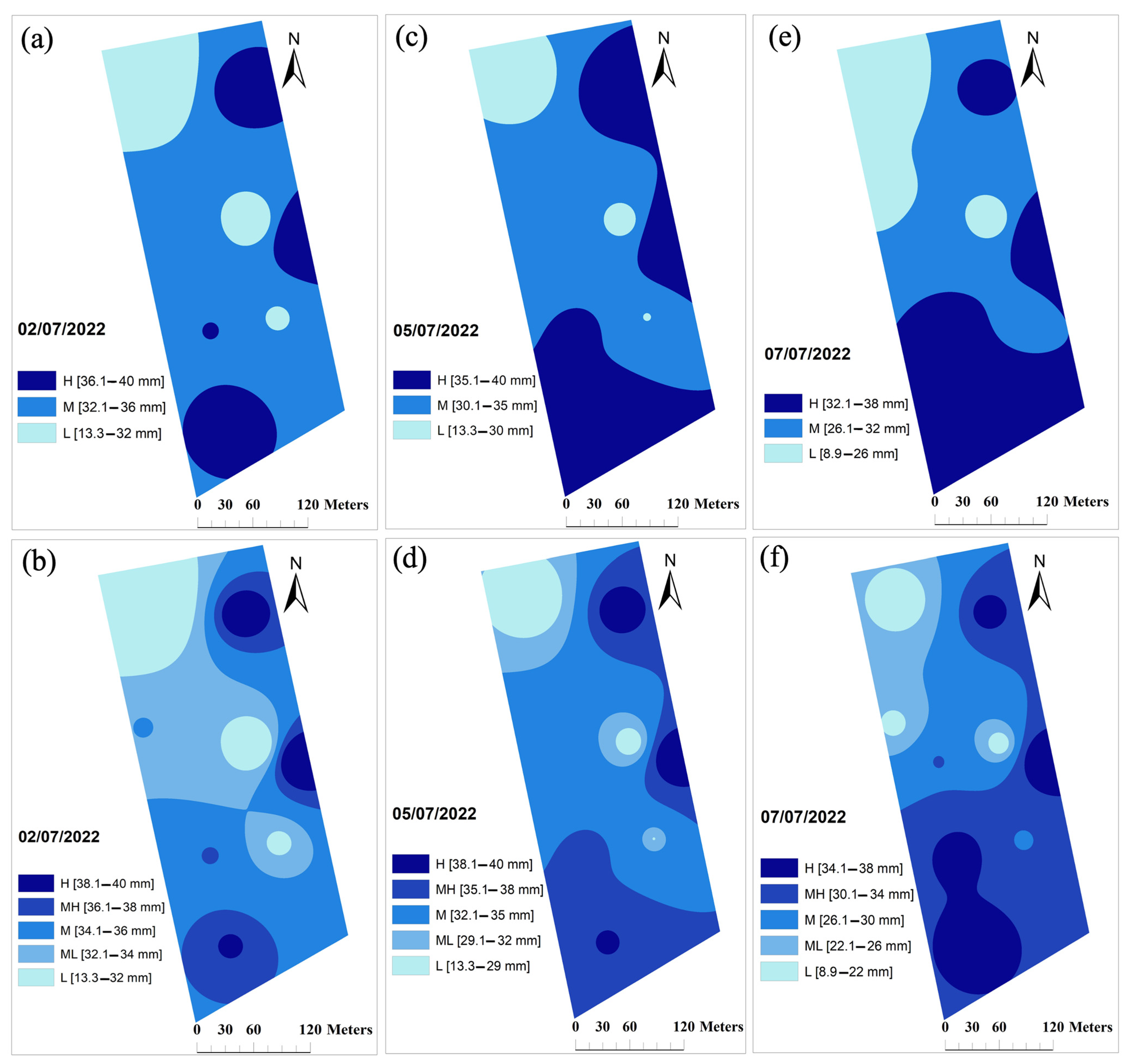
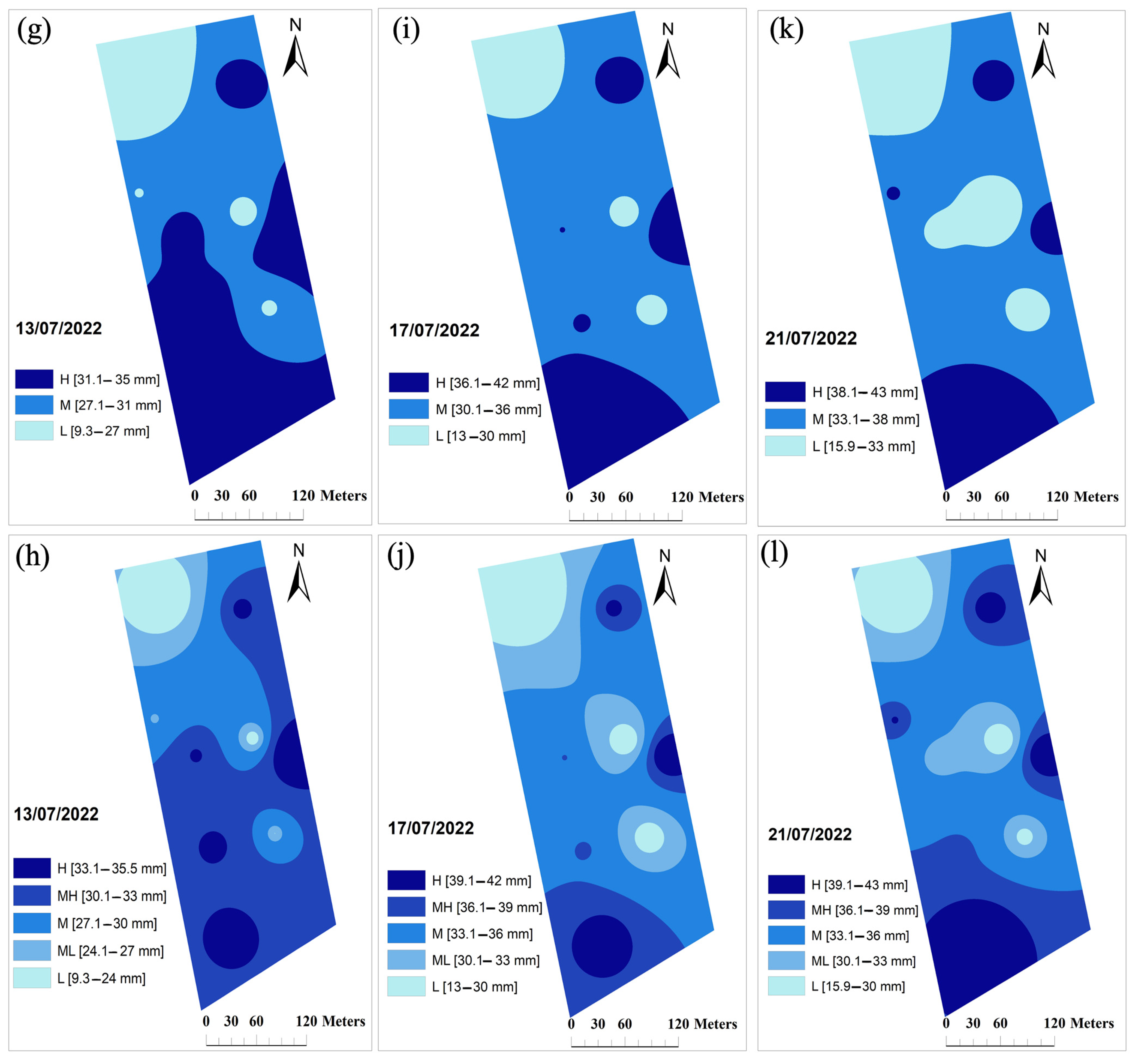
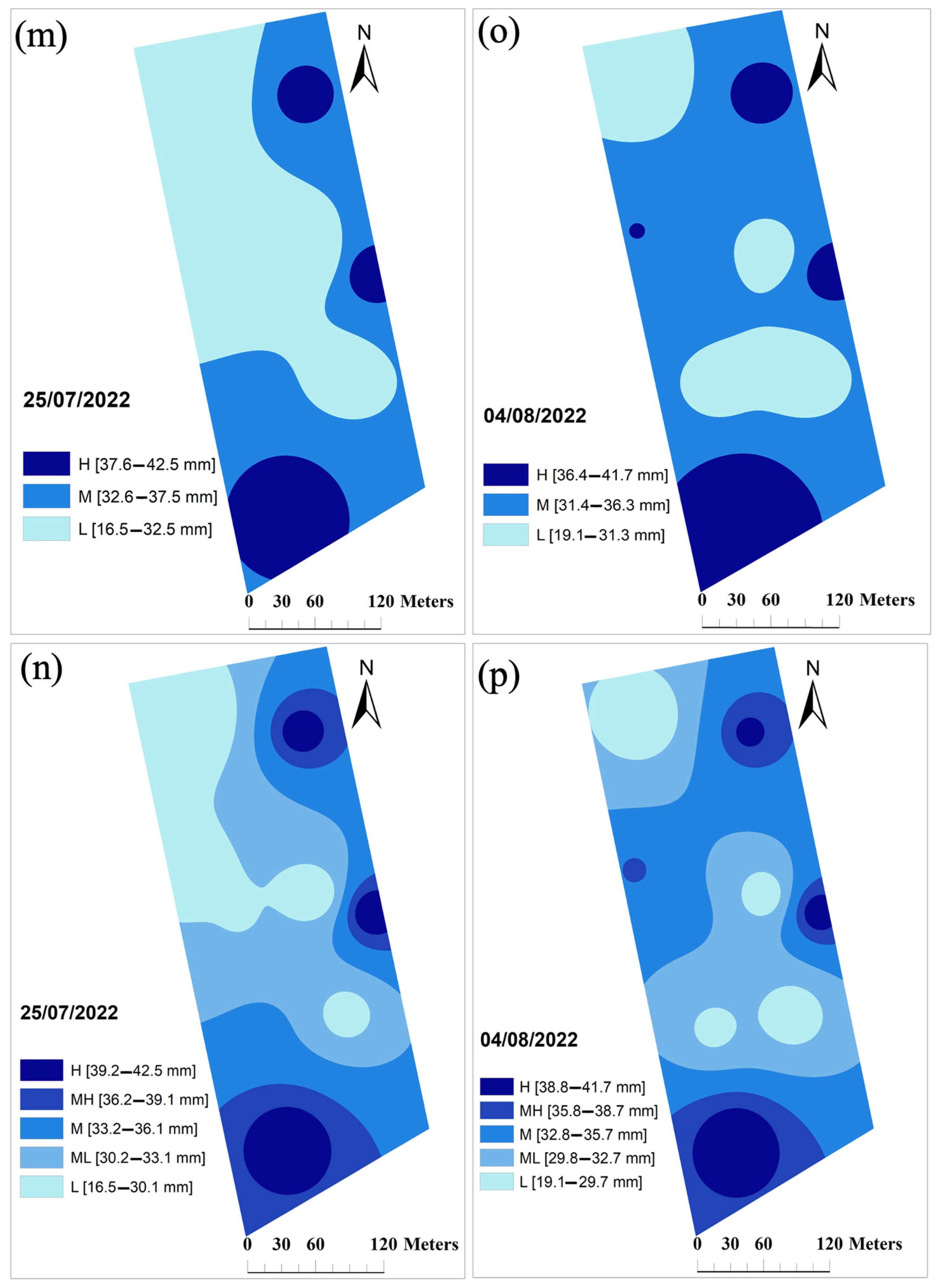
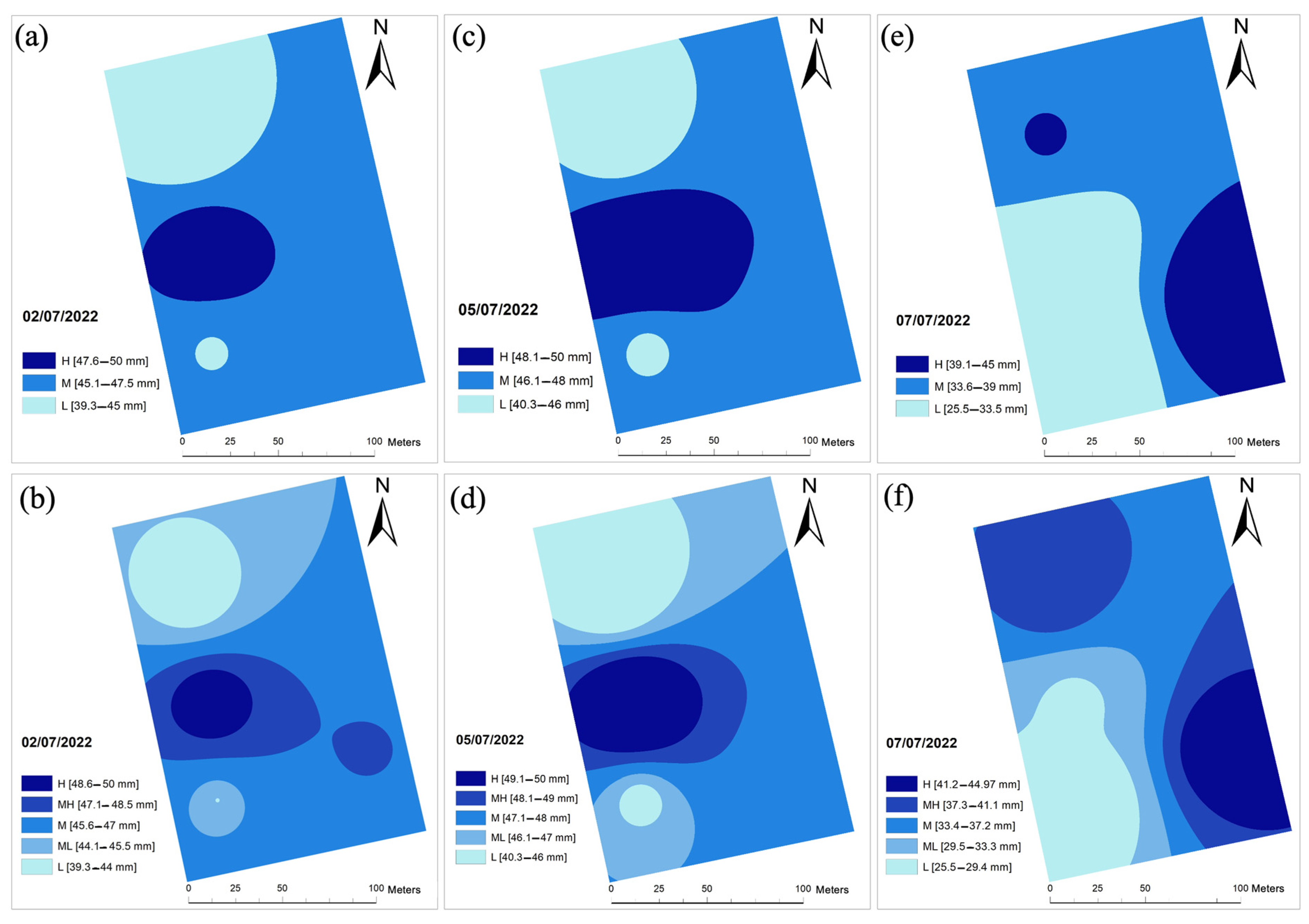
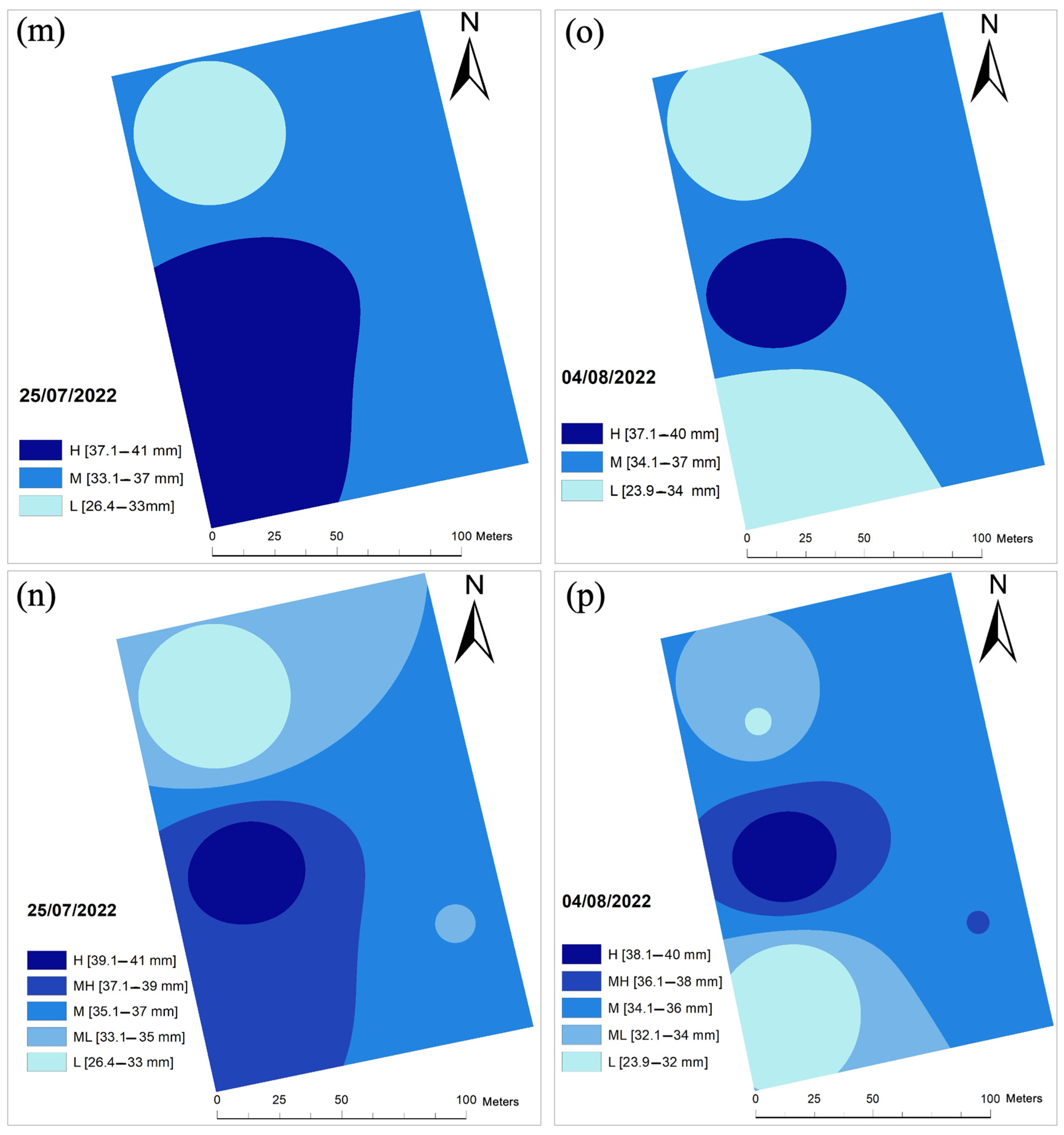
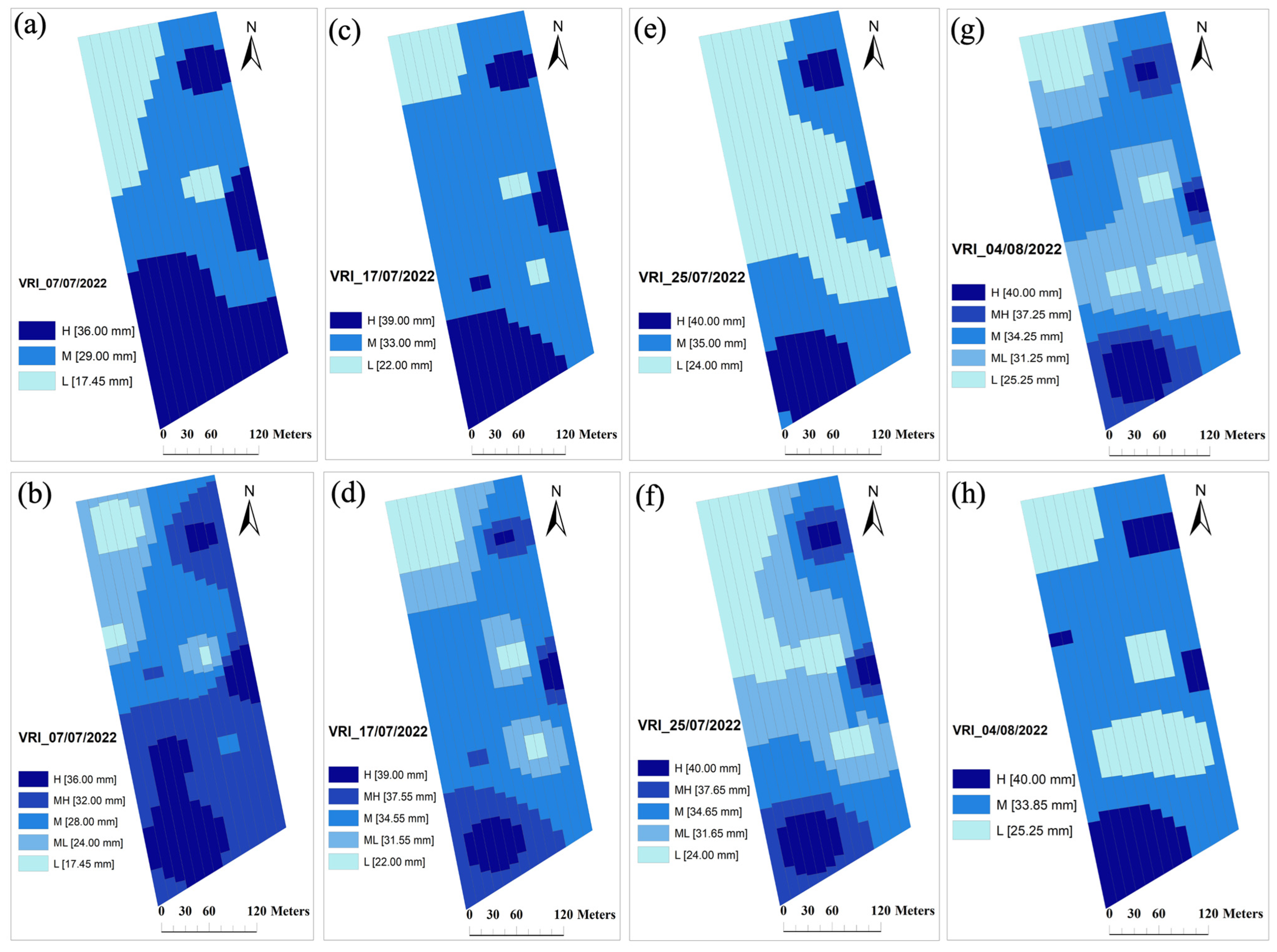
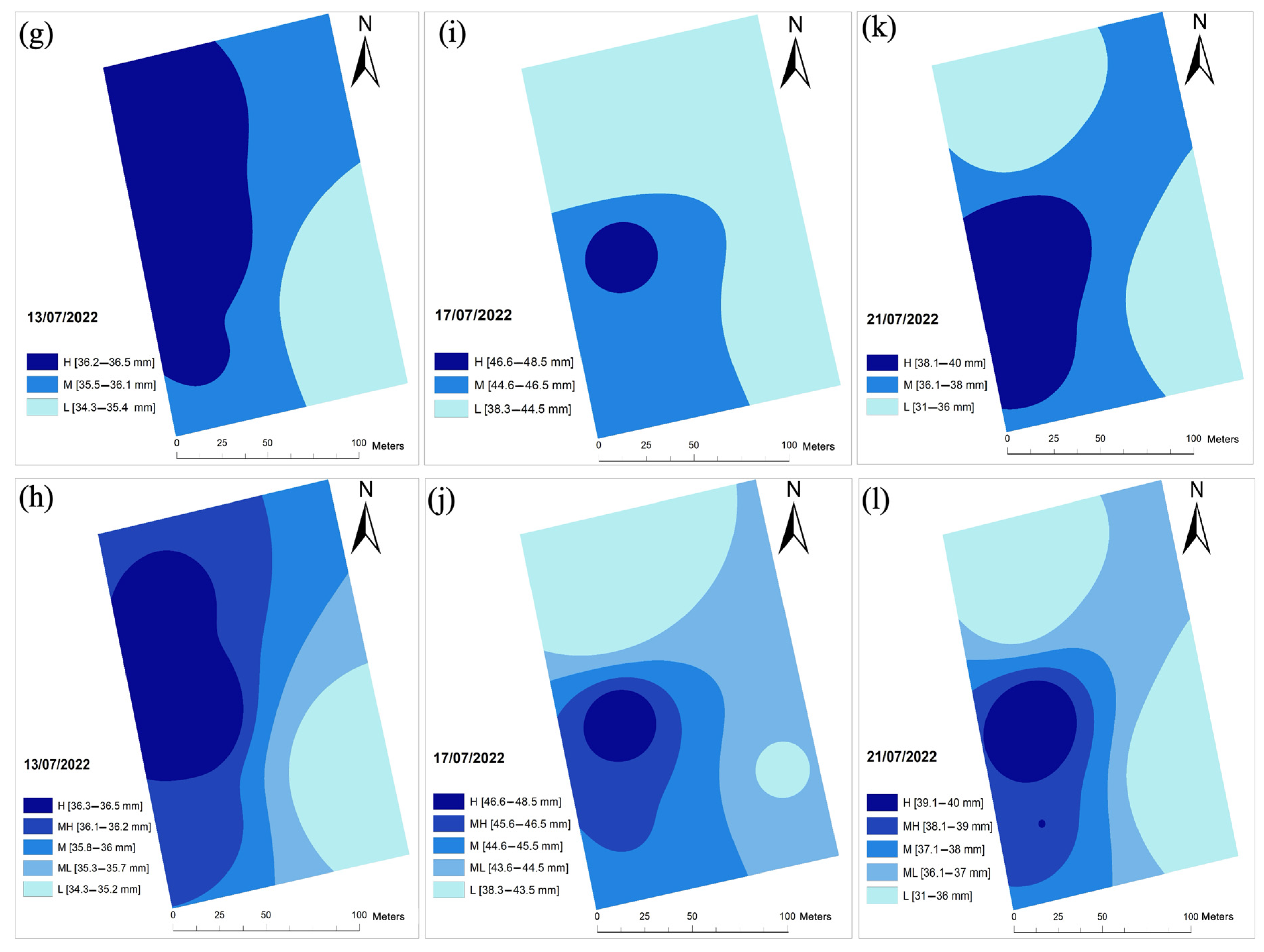
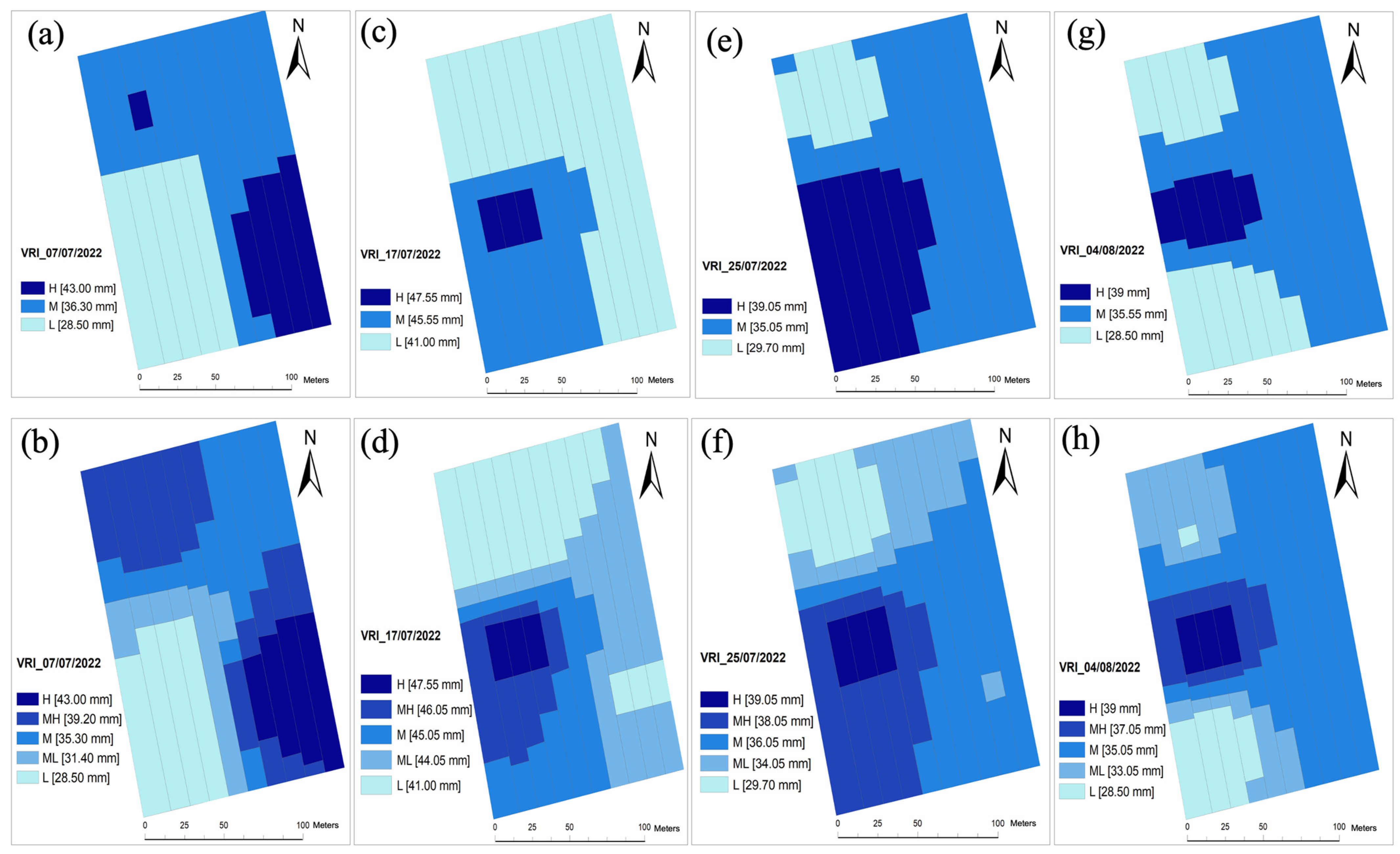
3.3. VRI Maps for Hose Reel Irrigation Machine

Since an irrigation system in a fixed-size management zone is unlikely to respond accurately to spatiotemporal irrigation needs, a linearly moving hose reel irrigation system with section control was proposed as a solution in this study. For a four-section control machine, the IN maps were translated into grid maps so that the hose reel irrigation machine could achieve a lateral application resolution of 11.5 m (with a working width of 46 m) and a longitudinal resolution with sub-meters due to the low ground speeds (30–80 m h⁻¹). Management zones with appropriate section widths that can be utilized by the VRFM are shown in Figure 6 for four selected irrigation days, both with three- and five-zone mapping.

Figure 6 and Figure 7 show that the ideal irrigation management zones present in Figure 4 and Figure 5, respectively, have to be changed due to the overlaps among the intersecting management zones when cells are formed with a width of 11.5 m with varying lengths. The lateral and longitudinal resolutions of the machine and the number of zones will be the initial determinants for the overall precision of the variable-rate irrigation application.

Table 7. Area (ha) of each variable rate irrigation (VRI) management zone for VRFM for Field 1 and Field 2.

		3 MZs			5 MZs
	Irrigation Date/Rate	H	M	L	H	MH	M	ML	L
F1	2 July	1.61	5.35	1.32	0.41	1.16	3.05	2.35	1.32
	5 July	3.16	4.31	0.82	0.49	2.68	3.78	0.67	0.66
	7 July	3.25	3.44	1.60	1.49	3.24	1.98	1.13	0.45
	13 July	3.67	3.44	1.18	0.81	4.11	2.18	0.55	0.64
	17 July	1.88	5.46	0.94	0.53	1.30	4.08	1.42	0.95
	21 July	1.60	4.84	1.85	1.22	1.77	3.48	1.11	0.70
	25 July	1.22	3.04	4.03	0.67	1.08	2.10	2.41	2.02
	4 August	1.44	4.84	2.00	0.62	1.02	2.96	2.65	1.02
	Ave.	2.23	4.34	1.72	0.78	2.05	2.95	1.54	0.97
	Std dev.	0.96	0.93	1.02	0.38	1.16	0.80	0.83	0.50
	%CV	43.32	21.54	59.59	48.84	56.80	27.21	53.71	52.15
F2	2 July	0.28	1.68	0.54	0.12	0.41	1.23	0.42	0.33
	5 July	0.53	1.49	0.49	0.29	0.24	0.94	0.55	0.49
	7 July	0.49	1.22	0.80	0.35	0.71	0.62	0.29	0.53
	13 July	1.05	0.86	0.60	0.58	0.70	0.49	0.28	0.45
	17 July	0.12	0.86	1.52	0.11	0.34	0.53	0.77	0.76
	21 July	0.57	0.96	0.98	0.23	0.32	0.30	0.67	0.98
	25 July	0.79	1.38	0.33	0.14	0.64	0.97	0.42	0.33
	4 August	0.25	1.50	0.76	0.12	0.26	1.35	0.48	0.29
	Ave.	0.51	1.24	0.75	0.24	0.45	0.80	0.49	0.52
	Std dev.	0.30	0.32	0.37	0.16	0.20	0.38	0.17	0.24
	%CV	59.82	25.77	49.26	67.40	44.30	46.99	35.12	46.14

L, low; ML, medium-low; M, medium; MH, medium-high; H, high.

provides the updated sub-areas of each management zone after the maps were fitted to the widths of the sections of the VRFM. When rectangular cells with fixed widths and varying lengths were used, the total area of each management zone changed accordingly. For instance, three-zone H-level application areas for F1 ranged from 1.22 ha to 3.67 ha for different irrigation dates, which were 0.90 ha to 3.26 ha in Table 6. For F2, L-level areas with five-zone analysis ranged from 0.29 ha (4 August) to 0.98 ha (21 July) in Table 7, whereas these areas were 0.27 ha and 0.99 ha, respectively for 4 August and 21 July in Table 6. In terms of the variations among irrigation days, the CV values were high in the application maps fitted to the VRF machine, ranging from 25.77 to 67.4%.

The means of three-zone areas for H, M, and L levels were 2.22, 4.34, and 1.71 ha in Field 1 and 0.50, 1.24, 1.24, and 0.75 ha in Field 2. The large area differences among the zones show that the constant-rate applications introduce large errors in the application rates. Similar evaluations can be performed for a specific irrigation date. For instance, five-zone areas corresponding to 17 July in F1 range from 0.53 ha (H level) to 4.1 ha (M level) with the largest area, showing up to eight-fold difference in area between different zones. It is documented in the literature that precision agriculture has the potential to reduce the excess amount of inputs in production agriculture, along with an increase in profit and energy saving [41,42]. Ref. [43] found large irrigation need differences within a study field, with a water requirement of up to 26% less in the management zones compared to user-rate applications and suggested that sensor-based variable-rate irrigation scheduling would prevent users from applying over- or under-irrigation.

Neither variations in NDVI nor the soil texture seemed to explain the sharp spatial or temporal changes in irrigation needs in this study. From visual comparisons, Figure 8 and Figure 9 could not reveal insight about the reasons for varying irrigation MZs within the field since there was no sign of correlation between the variations in MZs and NDVI or soil texture. Previous research has also concluded that NDVI data alone are not sufficient to make decisions in irrigation management [44]. More data, such as spatial emergence rate, plant density, leaf area index, and pest (weed and disease) pressure on plant growth, may reveal the necessary information to explain the cause of varying irrigation management zones.

The application rates associated with the dynamic management zones simulated in this study were based on measurements using multiple number of soil moisture sensors installed in fields integrated with a cloud-based wireless system. A greater number of sensors may improve the accuracy of application maps, albeit at a higher cost. A limitation of this study was to utilize only the MC data. Some researchers have utilized areal measurements, particularly NDVI, to reduce the daily soil moisture variance [20,45] and/or to develop a smart system for linear irrigation systems, whereas others have focused on individual sprinkler control in continuously moving irrigation systems [46,47,48,49,50]. Artificial intelligence (AI) techniques have been used to improve the decision-support process in irrigation scheduling [51,52,53,54].

4. Conclusions

Determining the dynamic irrigation MZs, and hence the instantaneous irrigation needs in a given field is of utmost importance to optimize water use within the fields. In this study, the irrigation needs of two maize fields were determined based on spatiotemporal soil moisture content variations using LoRaWAN-based soil moisture sensor technology in an attempt to simulate the dynamic irrigation management zones to be used with a hose reel irrigation machine. Wireless soil MC monitoring technology enabled the determination of accurate timing and rates for irrigation to meet the field capacity requirement. Simulations showed that management zones changed temporally within the fields, requiring an update of the irrigation map for the next irrigation. It was demonstrated that resolutions of the theoretical (contour) irrigation maps could be converted to applicable grids or cells to be used by advanced variable rate irrigation systems. A section-controlled variable rate hose reel irrigation machine (VRIM) is currently under development to implement the solution postulated in this study. Future work should adopt data fusion of weather, electrical conductivity (EC), leaf area index (LAI), and satellite thermal and NDVI data in an attempt to improve irrigation management zones for a variable rate hose reel irrigation system. Future irrigation scheduling methods should also focus on the management of soil moisture based on an advanced understanding of its effects on crop growth, either by integrating existing irrigation scheduling methods or developing new models using advanced algorithms.

References

1. Kalboussi, N.; Biard, Y.; Pradeleix, L.; Rapaport, A.; Sinfort, C.; Ait-Mouheb, N. Life cycle assessment as decision support tool for water reuse in agriculture irrigation. Sci. Total Environ. 2022, 836, 155486. [Google Scholar] [CrossRef]
2. Mrinmayi, G.; Bhagyashri, D.; Atul, V. A Smart Irrigation System for Agriculture Based on Wireless Sensors. Int. J. Innov. Res. Sci. Eng. Technol. 2016, 5, 6893–6899. [Google Scholar]
3. Gu, Z.; Qi, Z.; Burghate, R.; Yuan, S.; Jiao, X.; Xu, J. Irrigation scheduling approaches and applications: A review. J. Irrig. Drain. Eng. 2020, 146, 04020007. [Google Scholar] [CrossRef]
4. Plaščak, I.; Jurišić, M.; Radočaj, D.; Vujić, M.; Zimmer, D. An overview of precision irrigation systems used in agriculture. Teh. Glas. 2021, 15, 546–553. [Google Scholar] [CrossRef]
5. Zhang, H.; He, L.; Di Gioia, F.; Choi, D.; Elia, A.; Heinemann, P. LoRaWAN based internet of things (IoT) system for precision irrigation in plasticulture fresh-market tomato. Smart Agric. Technol. 2022, 2, 100053. [Google Scholar] [CrossRef]
6. Davcev, D.; Mitreski, K.; Trajkovic, S.; Nikolovski, V.; Koteli, N. IoT agriculture system based on LoRaWAN. In Proceedings of the 2018 14th IEEE International Workshop on Factory Communication Systems (WFCS), Imperia, Italy, 13–15 June 2018; IEEE: Piscataway, NJ, USA, 2018; pp. 1–4. [Google Scholar]
7. Zhang, Y.; Chen, D.; Wang, S.; Tian, L. A promising trend for field information collection: An air-ground multi-sensor monitoring system. Inf. Process. Agric. 2018, 5, 224–233. [Google Scholar] [CrossRef]
8. Haule, J.; Michael, K. Deployment of wireless sensor networks (WSN) in automated irrigation management and scheduling systems: A review. In Proceedings of the 2nd Pan African International Conference on Science, Computing and Telecommunications (PACT 2014), Arusha, Tanzania, 14–18 July 2014; IEEE: Piscataway, NJ, USA, 2014; pp. 86–91. [Google Scholar]
9. Hamami, L.; Nassereddine, B. Application of wireless sensor networks in the field of irrigation: A review. Comput. Electron. Agric. 2020, 179, 105782. [Google Scholar] [CrossRef]
10. Farooq, M.S.; Riaz, S.; Abid, A.; Umer, T.; Zikria, Y.B. Role of IoT technology in agriculture: A systematic literature review. Electronics 2020, 9, 319. [Google Scholar] [CrossRef]
11. Poblete-Echeverría, C.; Fuentes, S. Special Issue “Emerging Sensor Technology in Agriculture”. Sensors 2020, 20, 3827. [Google Scholar] [CrossRef]
12. Kumar, S.A.; Ilango, P. The impact of wireless sensor network in the field of precision agriculture: A review. Wirel. Pers. Commun. 2018, 98, 685–698. [Google Scholar] [CrossRef]
13. Jaynes, D.B.; Colvin, T.S. Spatiotemporal variability of corn and soybean yield. Agron. J. 1997, 89, 30–37. [Google Scholar] [CrossRef]
14. McBratney, A.X.; Whelan, B.M.; Shatar, T.M. Variability and uncertainty in spatial, temporal and spatiotemporal crop-yield and related data. In Ciba Foundation Symposium 210-Precision Agriculture: Spatial and Temporal Variability of Environmental Quality; John Wiley & Sons, Ltd.: Chichester, UK, 2007; pp. 141–160. [Google Scholar]
15. Cao, J.; Leng, G.; Yang, P.; Zhou, Q.; Wu, W. Variability in Crop Response to Spatiotemporal Variation in Climate in China, 1980–2014. Land 2022, 11, 1152. [Google Scholar] [CrossRef]
16. Ali, A.; Martelli, R.; Scudiero, E.; Lupia, F.; Falsone, G.; Rondelli, V.; Barbanti, L. Soil and climate factors drive spatio-temporal variability of arable crop yields under uniform management in Northern Italy. Arch. Agron. Soil Sci. 2023, 69, 75–89. [Google Scholar] [CrossRef]
17. O’Shaughnessy, S.A.; Evett, S.R.; Colaizzi, P.D.; Andrade, M.A.; Marek, T.H.; Heeren, D.M.; LaRue, J.L. Identifying advantages and disadvantages of variable rate irrigation: An updated review. Appl. Eng. Agric. 2019, 35, 837–852. [Google Scholar] [CrossRef]
18. Perry, C.; Podcknee, S. Development of a Variable-Rate Pivot Irrigation Control System. In Proceedings of the 2003 Georgia Water Resources Conference at the University of Georgia, Athens, GA, USA, 23–24 April 2003. [Google Scholar]
19. Vellidis, G.; Liakos, V.; Porter, W.; Tucker, M.; Liang, X. A Dynamic Variable Rate Irrigation Control System. In Proceedings of the 13th International Conference on Precision Agriculture, St. Louis, MO, USA, 31 July–4 August 2016. [Google Scholar]
20. Aleotti, J.; Amoretti, M.; Nicoli, A.; Caselli, S. A Smart Precision-Agriculture Platform for Linear Irrigation Systems. In Proceedings of the 2018 26th International Conference on Software, Telecommunications and Computer Networks (SoftCOM), Split, Croatia, 13–15 September 2018; IEEE: Piscataway, NJ, USA, 2022. [Google Scholar]
21. David, H.; Rakesh, V.S. Smart Irrigation Management System Using Lora Wan Based Sensor Nodes. Int. J. Appl. Eng. Res. 2020, 15, 2020. [Google Scholar]
22. Sharifnasab, H.; Mahrokh, A.; Dehghanisanij, H.; Łazuka, E.; Łagód, G.; Karami, H. Evaluating the Use of Intelligent Irrigation Systems Based on the IoT in Grain Corn Irrigation. Water 2023, 15, 1394. [Google Scholar] [CrossRef]
23. Briciu-Burghina, C.; Zhou, J.; Ali, M.I.; Regan, F. Demonstrating the potential of a low-cost soil moisture sensor network. Sensors 2020, 22, 987. [Google Scholar] [CrossRef]
24. Hossain, F.F.; Messenger, R.; Captain, G.L.; Ekin, S.; Jacob, J.D.; Taghvaeian, S.; O’Hara, J.F. Soil moisture monitoring through UAS-assisted internet of things LoRaWAN wireless underground sensors. IEEE Access 2022, 10, 102107–102118. [Google Scholar] [CrossRef]
25. Froiz-Míguez, I.; Lopez-Iturri, P.; Fraga-Lamas, P.; Celaya-Echarri, M.; Blanco-Novoa, Ó.; Azpilicueta, L.; Fernández-Caramés, T.M. Design, implementation, and empirical validation of an IoT smart irrigation system for fog computing applications based on Lora and Lorawan sensor nodes. Sensors 2020, 20, 6865. [Google Scholar] [CrossRef]
26. Sánchez-Sutil, F.; Cano-Ortega, A. Smart control and energy efficiency in irrigation systems using LoRaWAN. Sensors 2021, 21, 7041. [Google Scholar] [CrossRef] [PubMed]
27. Krishnan, S.R.; Nallakaruppan, M.K.; Chengoden, R.; Koppu, S.; Iyapparaja, M.; Sadhasivam, J.; Sethuraman, S. Smart Water Resource Management Using Artificial Intelligence—A Review. Sustainability 2022, 14, 13384. [Google Scholar] [CrossRef]
28. Turker, U.; Erdem, T.; Tagarakis, A.; Fountas, S.; Mitev, G.; Akdemir, B.; Gemtos, T.A. A Feasibility Study of Variable Rate Irrigation in Black Sea Area: Water and Energy Saving from the Application. J. Inf. Technol. Agric. 2011, 4, 1–6. [Google Scholar]
29. Liang, Z.; Liu, X.; Xiao, J.; Liu, C. Review of conceptual and systematic progress of precision irrigation. Int. J. Agric. Biol. Eng. 2021, 14, 20–31. [Google Scholar] [CrossRef]
30. Yabacı, S.H. Variable Rate Irrigation System Developing on Hose Reel Type Irrigation Systems. Ph.D. Thesis, Tekirdağ Namık Kemal University, Tekirdağ, Türkiye, 2022. (In Turkish). [Google Scholar]
31. Awawda, J.; Ishaq, I. IoT Smart Irrigation System for Precision Agriculture. In Intelligent Sustainable Systems: Selected Papers of WorldS4 2022; Springer Nature: Singapore, 2023; Volume 2, pp. 335–346. [Google Scholar]
32. Gundim, A.D.S.; Melo, V.G.M.L.D.; Coelho, R.D.; Silva, J.P.D.; Rocha, M.P.A.D.; França, A.C.F.; Conceição, A.M.P.D. Precision irrigation trends and perspectives: A review. Ciência Rural 2023, 53, 8. [Google Scholar] [CrossRef]
33. Bantchina, B.B.; Mucan, U.; Gündoğdu, K.S. Land availability analysis in Bursa using Geographic Information Systems. In Proceedings Book, Proceedings of the 5th International Participation Soil and Water Resources Congress, Kırklareli, Turkey, 12–15 September 2017; Atatürk Soil Water and Agricultural Meteorology Research Institute Kırklareli: Merkez, Turkey, 2017; Volume 1, pp. 65–74. [Google Scholar]
34. Dragino LSE01-LoRaWAN Soil Moisture & EC Sensor User Manual. Available online: https://www.dragino.com/products/agriculture-weather-station/item/277-se01-lb.html (accessed on 17 June 2023).
35. El-Naggar, A.G.; Hedley, C.B.; Horne, D.; Roudier, P.; Clothier, B.E. Soil sensing technology improves application of irrigation water. Agric. Water Manag. 2020, 228, 105901. [Google Scholar] [CrossRef]
36. Irmak, S.; Rees, J.M.; Zoubek, G.L.; van DeWalle, B.S.; Rathje, W.R.; DeBuhr, R.; Leininger, D.; Siekman, D.D.; Schneider, J.W.; Christiansen, A.P. Nebraska agricultural water management demonstration network (NAWMDN): Integrating research and extension/outreach. Appl. Eng. Agric. 2010, 26, 599–613. [Google Scholar] [CrossRef]
37. Allen, R.G.; Pereira, L.S.; Raes, D.; Smith, M. Crop Evapotranspiration-Guidelines for Computing Crop Water Requirements-FAO Irrigation and Drainage Paper 56; FAO: Rome, Italy, 1998. [Google Scholar]
38. World Bank. Reengaging in Agricultural Water Management. Challenges and Options; The World Bank: Washington, DC, USA, 2006. [Google Scholar]
39. Tucker, C.J. Red and photographic infrared linear combinations for monitoring vegetation. Remote Sens. Environ. 1979, 8, 127–150. [Google Scholar] [CrossRef]
40. Da Cunha Leme Filho, J.F.; Ortiz, B.V.; Damianidis, D.; Balkcom, K.S.; Dougherty, M.; Poschel, T. Irrigation scheduling to promote corn productivity in central Alabama. J. Agric. Sci. 2020, 12, 34–51. [Google Scholar]
41. Gao, Y.; Duan, A.; Qiu, X.; Liu, Z.; Sun, J.; Zhang, J.; Wang, H. Distribution of roots and root length density in a maize/soybean strip intercropping system. Agric. Water Manag. 2010, 98, 199–212. [Google Scholar] [CrossRef]
42. Souza, S.A.; Rodrigues, L.N. Increased profitability and energy savings potential with the use of precision irrigation. Agric. Water Manag. 2022, 270, 107730. [Google Scholar] [CrossRef]
43. Vories, E.; O’Shaughnessy, S.; Sudduth, K.; Evett, S.; Andrade, M.; Drummond, S. Comparison of precision and conventional irrigation management of cotton and impact of soil texture. Precis. Agric. 2021, 22, 414–431. [Google Scholar] [CrossRef]
44. Bondesan, L.; Ortiz, B.V.; Morlin, F.; Morata, G.; Duzy, L.; van Santen, E.; Vellidis, G. A comparison of precision and conventional irrigation in corn production in Southeast Alabama. Precis. Agric. 2023, 24, 40–67. [Google Scholar] [CrossRef]
45. Quebrajo, L.; Perez-Ruiz, M.; Perez-Urrestarazu, L.; Martinez, G.; Egea, G. Linking thermal imaging and soil remote sensing to enhance irrigation management of sugar beet. Biosyst. Eng. 2017, 165, 77–87. [Google Scholar] [CrossRef]
46. Fontanet, M.; Scudiero, E.; Skaggs, T.H.; Fernàndez-Garcia, D.; Ferrer, F.; Rodrigo, G.; Bellvert, J. Dynamic management zones for irrigation scheduling. Agric. Water Manag. 2020, 238, 106207. [Google Scholar] [CrossRef]
47. Jimenez, A.F.; Cardenas, P.F.; Canales, A.; Jimenez, F.; Portacio, A. A survey on intelligent agents and multi-agents for irrigation scheduling. Comput. Electron. Agric. 2020, 176, 105474. [Google Scholar] [CrossRef]
48. Reyes, J.; Wendroth, O.; Matocha, C.; Zhu, J. Delineating Site-Speciic Management Zones and Evaluating Soil Water Temporal Dynamics in a Farmer’s Field in Kentucky. Vadose Zone J. Adv. Crit. Zone Sci. 2019, 18, 1–19. [Google Scholar] [CrossRef]
49. Kim, Y.; Evans, R.G.; Iversen, W.M. Remote sensing and control of an irrigation system using a distributed wireless sensor network. IEEE Trans. Instrum. Meas. 2008, 57, 1379–1387. [Google Scholar]
50. Chavez, J.L.; Pierce, F.J.; Elliott, T.V.; Evans, R.G. A remote irrigation monitoring and control system for continuous move systems. Part A: Description and development. Precis. Agric. 2010, 11, 1–10. [Google Scholar] [CrossRef]
51. Al-Qammaz, A.; Darabkh, K.A.; Abualigah, L.; Khasawneh, A.M.; Zinonos, Z. An AI-based irrigation and weather forecasting system utilizing LoraWAN and cloud computing technologies. In Proceedings of the 2021 IEEE Conference of Russian Young Researchers in Electrical and Electronic Engineering (ElConRus), Moscow, Russia, 26–29 January 2021; IEEE: Piscataway, NJ, USA, 2021; pp. 443–448. [Google Scholar]
52. Talaviya, T.; Shah, D.; Patel, N.; Yagnik, H.; Shah, M. Implementation of artificial intelligence in agriculture for optimisation of irrigation and application of pesticides and herbicides. Artif. Intell. Agric. 2020, 4, 58–73. [Google Scholar] [CrossRef]
53. Muangprathub, J.; Boonnam, N.; Kajornkasirat, S.; Lekbangpong, N.; Wanichsombat, A.; Nillaor, P. IoT and agriculture data analysis for smart farm. Comput. Electron. Agric. 2019, 156, 467–474. [Google Scholar] [CrossRef]
54. Perea, R.G.; Poyato, E.C.; Montesinos, P.; Díaz, J.R. Prediction of applied irrigation depths at farm level using artificial intelligence techniques. Agric. Water Manag. 2018, 206, 229–240. [Google Scholar] [CrossRef]
Figure 1. Study site (Field 1 and Field 2) with fields sub-plots for the drip irrigation.
Soilsystems 08 00019 g001
Figure 2. LoRaWAN used for continuous soil moisture data collection [34].
Soilsystems 08 00019 g002
Figure 3. The soil moisture content (MC) before irrigation (BI) and after irrigation (AI) and their relationship with field capacity average (FC_Ave), permanent point average (PWP_Ave), and management allowable depletion (MAD) for Field 1 (a) and Field 2 (b).
Soilsystems 08 00019 g003
Figure 4. Three and five irrigation management zones maps for Field 1 for different irrigation dates in 2022: (a,b), 2 July; (c,d), 5 July; (e,f), 7 July; (g,h), 13 July; (i,j), 17 July; (k,l), 21 July; (m,n), 25 July; and (o,p), 4 August.
Soilsystems 08 00019 g004aSoilsystems 08 00019 g004bSoilsystems 08 00019 g004c
Figure 5. Three and five irrigation management zones maps for Field 2 for different irrigation dates in 2022: (a,b), 2 July; (c,d), 5 July; (e,f), 7 July; (g,h), 13 July; (i,j), 17 July; (k,l), 21 July; (m,n), 25 July; and (o,p), 4 August.
Soilsystems 08 00019 g005aSoilsystems 08 00019 g005bSoilsystems 08 00019 g005c
Figure 6. Three and five-MZs maps for VRI using VRFM for Field 1 on selected irrigation days in 2022: (a,b), 7 July; (c,d), 17 July; (e,f), 25 July; and (g,h), 4 August.
Soilsystems 08 00019 g006
Figure 7. Three- and five-MZs maps for VRI using VRFM for Field 2 onselected irrigation days in 2022: (a,b), 7 July; (c,d), 17 July; (e,f), 25 July; and (g,h), 4 August.
Soilsystems 08 00019 g007
Figure 8. NDVI for a given dates (ag) and soil texture (sand, silt, and clay) (hj) maps for Field 1.
Soilsystems 08 00019 g008
Figure 9. NDVI for given dates (ag) and soil texture (sand, silt, and clay) (hj) maps for Field 2.
Soilsystems 08 00019 g009