Spatial Variability of Soil Erodibility at the Rhirane Catchment Using Geostatistical Analysis

Abstract

Soil erodibility is one of the most crucial factors used to estimate soil erosion by applying modeling techniques. Soil data from soil maps are commonly used to create maps of soil erodibility for soil conservation planning. This study analyzed the spatial variability of soil erodibility by using a digital elevation model (DTM) and surface soil sample data at the Rhirane catchment (Algeria). A total of 132 soil samples were collected of up to 20 cm in depth. The spatial distributions of the K-value and soil physical properties (permeability, organic matter, and texture) were used to elaborate ordinary Kriging interpolation maps. Results showed that mean values of soil organic matter content were statistically different between Chromic Cambisols (M = 3.4%) vs. Calcic Cambisols (M = 2.2%). The analysis of variance of the organic matter provided a tool for identifying significant differences when comparing means between the soil types. The soil granulometry is mainly composed of silt and fine sand. The soil erodibility showed values varying between 0.012 and 0.077 with an average of 0.034, which was greater in soils with calcic horizons. Statistical evaluation by using Pearson’s correlation revealed positive correlations between erodibility and silt (0.63%), and negative correlations with sand (−0.16%), clay (−0.56%), organic matter (−0.32%), permeability (−0.41%), soil structure (−0.40%), and the soil stability index (−0.26%). The variability analysis of the K-factor showed moderate spatial dependency with the soil erodibility map indicating moderate to highly erodible risk in cropland and sparse grassland land uses. Overall, the study provides scientific support for soil conservation management and appropriate agricultural food practices for food supply.

1. Introduction

Soil erosion is a gradual process that occurs when water and/or wind detaches and removes soil particles. When geological or natural erosion occurs, it is considered as a crucial component of the natural evolution of the physical ecosystem and the creation of landscapes [1]. The inherent features of soil, such as erodibility, are one of the most important and effective parameters in considering soil erosion.

Soil erodibility is subjected to temporal and spatial variability, and relates to how easily soil may be washed away by surface flow, splash during rainfall, or both; making it one of the key signs of land degradation.

The most critical resource for providing food to humans is soil productivity. Furthermore, due to the growing population and the intensification of agricultural practices, loss of this productive capability, along with rising soil erosion rates, has become a socioeconomic challenge. Consequently, the improvement of erosion control management techniques, for a better understanding of soil erosion dynamics and soil loss prediction, has increased attention [2].

In order to control soil erosion, it is imperative to apply measures for the conservation and management of natural resources to prevent water erosion and to obtain information on soil erosion methods based on an accurate assessment of vulnerability and risk levels. Predicting soil erosion susceptibility and verifying the primary sources of erosion in a given area are the first steps in determining appropriate erosion control techniques [1,2,3].

Traditional soil surveys are created using a three-step method represented by a scheme that consists of three major components defined by a model employing a similarity representation of soils, a set of inference techniques for deriving the similarity representation, and the use of the similarity representation [4]. Over the past decade, researchers have been interested in inputting soil data into predictive environmental models, which cannot be carried out reliably using overly generalized maps due to their qualitative nature. Recent advances in mapping technology such as remote sensing, geographic information systems, and terrain modeling via surveys, geometrics, and geospatial approaches, for example, provide options to conduct more thorough and precise soil erosion studies [5].

The soil erodibility or K-factor is an essential parameter in erosion prediction and soil conservation management. Soil factors such as texture, organic matter, permeability, and soil structure influence soil erodibility [6].

The quantity of soil loss by runoff, rainwater, or seepage inside a common unit is known as the K-factor, which is used to measure soil erodibility in the universal soil loss equation (USLE) and revised universal soil loss equation (RUSLE) [7]. For K-factor determination, two primary approaches have been introduced. The first approach, which is time-consuming and expensive but yields the best soil erodibility (K) assessment in reality, involves directly measuring the K-factor from standard plots [8]. A second approach is based on the USLE nomograph derived from Wischmeier et al. [9] and Wischmeier and Smith [10], who found good correlations between the K-factor and a few chosen soil parameters, and is widely used to estimate the K-factor [7].

Numerous studies have been conducted using the K-factor to predict soil loss. Wang et al. [11] assessed and compared soil erodibility and discovered the accuracy of the K-value obtained from soil erodibility prediction maps by using the soil survey of Coryell County in Texas (USA) and soil erodibility values driven from a set of soil samples. Bahrami et al. [12] developed a method for obtaining the K-factor as an output by utilizing the soil characteristics as inputs and demonstrating the system’s applicability by comparing them with the K-values calculated with the USLE model. Vaezi et al. [13] employed the USLE nomograph to predict the K-factor in the northwest of Iran, as well as direct field measurements of the rate of soil loss from runoff plots. They found that the nomograph would overestimate the soil erodibility in the study area. Auerswald et al. [3] argued that USLE nomograph provides a high standard for measuring soil erodibility but within this complex equation exists a potential error. They developed a set of equations that expand on Wischmeier and Smith’s K-factor equation [10] by considering extreme values in silt content, soil erodibility, organic matter, and rock fragments. Blake et al. [14] worked in this sense in Australian soils affected by fires. Wang et al. [7] assessed the performance of available soil erodibility estimators from the Universal Soil Loss Equation (USLE), the Revised Universal Soil Loss Equation (RUSLE), the Erosion Productivity Impact Calculator (EPIC), and the Geometric Mean Diameter (Dg) model for different geographic regions based on Chinese soil loss data.

Few studies were oriented towards determining soil erodibility in relation to the agricultural practices and the slope of the terrain to suggest managing strategies in Algeria. Tubal et al. [15] estimated and mapped soil losses in the Wadi Sahou basin in the northwest of Algeria by using the Revised Universal Soil Loss Equation (RUSLE) model assisted by a Geographic Information System (GIS) and remote sensing data. According to Marques et al. [16], one of the alternatives to measure the K factor is derived from direct measurements in experimental fields under natural or simulated rain; however, under these conditions the estimation becomes costly and time-consuming, even considering the standard method [17]. To improve the geographic resolution of the K-factor map, further values of the K-factor can be assessed using a double rings infiltration test and assessments of soil physical–chemical parameters. [17]. Using Kriging interpolation, Liu et al. [6] investigated the features of the distribution of the K-factor erodibility in a limited basin in the Dan River watershed, China. In such a way, the application of this type of methodology can give results that would be applied worldwide.

Under these considerations, the objectives of this research were: (i) exploration of soil erodibility through the USLE method by utilizing alternate sources of soil sample information; (ii) correlation between the soil erodibility factor and soil physical properties; and (iii) characterization and mapping of the spatial variability of selected physical soil properties and soil erodibility in order to ascertain areas prone to erosion for sustainable land use and soil resources.

2. Materials and Methods

2.1. Study Area

One of the sub-basins of the Mellah basin is the Rhirane catchment, and its major stream is a tributary of the R’biba Wadi which, with the Bourdine Wadi, forms the main river called Mellah Wadi. The study area has an elongated shape with a northwest–southeast orientation and occupies an area of 80.82 km². The topography of the catchment, determined using a digital elevation model (DTM) with a spatial resolution of 30 m (SRTM 1 s arc), shows that the elevation of the basin varies between 302 m and 1277 m (Figure 1). The hydrographic system of the Rhirane Wadi originates in a mountainous relief and is composed of Guelala Hill (1243 m), Mekmen Hill (1287 m), Ras el Arous Hill (1156 m), and el Koukez Hill (1033 m).

The region is influenced by a Mediterranean climate with a marked wet season (December to April), long rainy periods (January to March), and a low rainfall in the summer season. The mean annual precipitation is equal to 644 mm (based on the period 1981 to 2019). The intensity and duration of rainfall is very significant in the form of short and high storms. Moreover, early rainstorms exceed 30 mm/h in November, and December to March [18].

The bedrocks are typically marly limestone of Eocene (21 km² of the basin area), and sandstone (Oligocene), limestone and marly (Cretaceous), and gypsum clay (Triassic), and their distribution varies from 10.44 to 11.25 km². The quaternary formation (21 km²) is spread over the entire basin area. The dominant soils are mainly Calcic Cambisols (Bk, covering 75% of the area), Chromic Cambisols (Bc), and Leptosols [19,20].

The Rhirane catchment is characterized by a heterogeneous rugged terrain dominated by steep slopes where 71% of the basin hillslopes exceed 15% of the slope, which exposes the basin landform to high erosion. The vegetation of the area consists mainly of crops (39%), and the southeast region is covered by grasslands and sparse shrubs. Shrubs and rangelands predominate in the eastern part of the basin, which frequently has a moderately sloping surface. The western, central, and northern regions are occupied by sparse shrubs and crops.

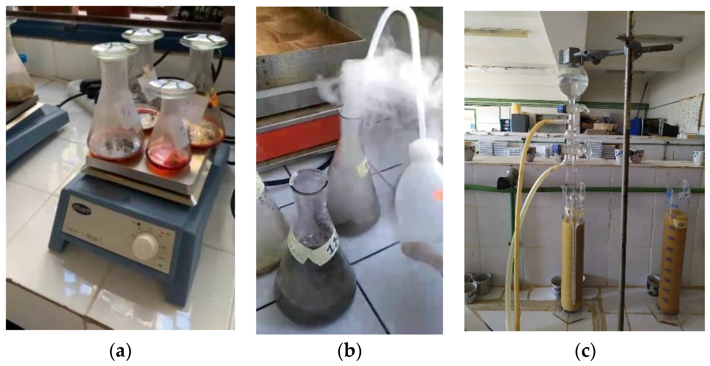
2.2. Soil Sampling and Soil Erodibility Estimation

A field survey was conducted to evaluate the soil’s characteristics and assess its level of erodibility (Figure 2). A systematic random method was followed for field sampling during the years 2020 and 2021. A grid for the sampling work (750 m × 750 m) was established and a Garmin portable GPS (GPS map 62 stc) was used to record the geospatial information. For this study, 132 topsoil samples were collected with different vegetation types (associated with land cover) and slopes (0−20 cm soil depth). To determine how vegetation affects soil erodibility, three representative land cover types were selected: shrub, grassland, and cropland. The soil samples were transferred to the lab in polyethylene bags, dried at room temperature, and homogenized for sifting (fine earth, 2 mm).

Using HCl (0.5 mol/L) and 2.0 mol/L (KCL), respectively, carbonates and inorganic nitrogen (NO₃⁻ and NH₄⁺) from soil samples were removed (Figure 3b). The Walkley–Black technique (Figure 3a) was used to calculate organic carbon (dichromate oxidation) [21].

The conventional factor of 1.724, based on the assumption that soil organic matter contains 58% carbon, can be applied to convert soil organic carbon (SOC) into soil organic matter content (SOM) [22]. In this research, the SOC to SOM conversion factor was chosen.

Robinson’s pipette technique (Figure 3c) was utilized to determine granulometry and texture. According to the United States Department of Agriculture’s (USDA) classification standards for soil texture, sand, silt, and clay particle sizes were categorized as follows: 0.05–2.0 mm for sand, 0.002–0.05 mm for silt, and 0.002 mm for clay [23]. The K-factor could be calculated considering granulometry, SOM content, and permeability. The National Soils Handbook was used to calculate soil permeability, while the Soil Textural Triangle was used to evaluate soil structure [23]. The soil erodibility (K-factor) was determined by using the Wischmeier and Smith [10] and Renard et al. [24] models. The estimation of the USLE soil erodibility factor was calculated as follows:

$$K=\frac{2.173\times 2.1\times M^{1.14}\times \left(10-4\right)\times \left(12-OM\right)+3.25\times \left(st-2\right)+2.5\times (p-3)}{100}$$

(1)

where K represents the soil erodibility factor (t∙ha∙h∙ha⁻¹∙Mj⁻¹∙mm⁻¹); M denotes particle percentages (% of very fine sand + % of silt × (100–%clay)); OM is the organic matter content (% C × 2); st is the code for the soil’s granularity (very fine: 1–2 mm; fine: 2–5 mm; medium or coarse: 5–10 mm; and blocky, platy, or massive: >10 mm); p is the code for permeability (p = 1, high to very high (>12.5 cm/h); p = 2, moderate to high (6.25–12.5 cm/h); and p = 3, moderate (2–6.25 cm/h); p = 4).

There is a general knowledge that low SOM may affect soil physical properties and increase soil erodibility due to the reduction in the formation of the organic matter–clay complex and soil structure. The effects on soil physical properties can be related to the clay-size soil fraction too.

Apart from the prediction of the soil erodibility index, some other indices were also used by researchers to understand the proneness of soil to erosion. Pieri [25] developed the soil aggregate stability index or structural stability index (SSI) to assess soil structural degradation by using soil organic matter, clay, and silt contents. In other studies on soil fertility, Pieri [26] and Reynolds [27] introduced a modified SSI by using SOC as a substitute for SOM to measure soil risk to structural degradation and aggregate stability as follows:

$$\mathrm{S}\mathrm{S}\mathrm{I}=\frac{1.724\times \mathrm{SOC}}{\mathrm{Silt}+\mathrm{Clay}}\times 100$$

(2)

where SOC is the soil organic carbon (%); Silt + Clay is the soil’s combined silt and clay content (%); SSI > 9% indicates a stable structure with sufficient SOC to ensure main structural stability; the amount of 7% < SSI ≤ 9% indicates a low risk of structural degradation (which implies low risk of physical degradation); the amount of 5% < SSI ≤ 7% indicates a high risk of degradation and high hazard of physical degradation; and SSI ≤ 5% indicates structurally degraded soil, which indicates severe physical degradation.

2.3. Statistical and Spatial Analysis

2.3.1. Analysis of Variance

Descriptive statistics was applied to the soil data and Tukey’s method was used to analyze the dispersion of quartiles and to identify outliers.

The analysis of variance (one-way ANOVA) was applied to analyze each factor’s relationship with the K-value based on the level of significance [28], determining if the qualitative variable “soil type” affects the quantitative variables “K factor”, “Organic matter”, “Soil structure”, and “Soil permeability” by using Fisher’s test (F-distribution) with a threshold of significance of 5%. The XLSTAT 2018 program was used for computations.

F-distribution was used as the sampling distribution. We set the critical values and tested the hypothesis accordingly as follows: the null hypothesis was tested to establish if the means and the variances of the used samples are equal; if we rejected the null hypo-thesis that the means and variances of the samples are equal, then we are stating that the differences that we observed could not have happened only by chance.

There are several steps to perform the ANOVA test. They include the following calculations or equations:

$$S{b}^2=\frac{{\sum }_i^{c}ni{\left(\overline{y}i-\overline{y}\right)}^2}{c-1}$$

(3)

where:

Sb is the sum of the differences between the individual soils and the mean in each group.

i is the group number.

ni is the sample size of group i.

$\overline{y}i$ is the mean of group i.

$\overline{y}$ is the overall mean of all the observations.

c is the total number of groups.

The second equation is the within-groups variance:

$$S{w}^2=\frac{{\sum }_i^c{\sum }_j^{ni}{\left(yij-\overline{y}i\right)}^2}{N-c}$$

(4)

where:

the sum of yij is all the values of the observations within and between groups.

N is the total number of observations.

c is the total number of groups.

Then, we calculate the observed value of the F-distribution as:

$$Fobs=\frac{Sb²}{Sw²}$$

(5)

Once all the calculations are completed, the critical F* is determined from the F-distribution table with:

State the significance level of α = 0.05.

Obtain degrees of freedom.

df (nominator) = c − 1 = 2; df (denominator) = N − c = 129.

Using these values, the F* was read from the F-distribution table and the result was precisely equal to 3.07.

If F_obs > F*, we reject the null hypothesis which states that there is no difference between the soil types.

If F_obs < F*, we do not reject the null hypothesis but state that the sample is not significant evidence for detecting a relationship between the variables.

2.3.2. Spatial Analysis and Statistics

After the calculation of each sample’s K factor, to map erodibility, the ordinary Kriging approach was employed. The spatial data, soil properties, and K values needed to assess soil erodibility were treated with Geographic Information System (ArcGIS 10.4.1) software and statistical software (R). In order to obtain a prediction map of the erosion risks for soil systems, geostatistics is increasingly employed in conjunction with GIS. When making predictions at unsampled places and determining the degree of uncertainty in those predictions, geostatistical approaches employ the stochastic theory of spatial correlation. Kriging is one of the most frequently applied interpolation techniques, in general, and it estimates the value of variables over a continuous geographical area by using a small number of sampling data. It requires a mathematical model to describe the spatial covariance, usually expressed as a variogram (called a semivariogram), which in its parameterized form has become the central tool of geostatistics.

In geostatistics, the semivariogram, which is a measure of the strength of statistical correlation as a function of distance, is derived by applying the following equation for N pairs of values of soil property Z separated by a distance, h:

$$\mathsf{\gamma }\left(h\right)=\frac{1}{2N\left(h\right)}{\sum }_{i=1}^{N\left(h\right)}\left[Z\right(x_i)-Z(x_i+h){]}^2$$

(6)

where γ (h) is the average semivariance sample to the distance h, (x_i) and (x_i + h) are sampling locations separated by a distance, h. Z(x_i) and Z (x_i + h) are measured values of the variable Z at the corresponding locations. For the spatial autocorrelation process as defined by Addis et al. [29], the semivariogram model with the smallest reduced sum of squares (RSS) was used in this research. This is one of the finest criteria for parameter and model selection; the RSS assesses the total discrepancy between observed data and the estimated values by a prediction model [30].

The normal distribution of the dataset was tested by Kolmogorov–Smirnov analysis. Ordinary Kriging interpolation is often utilized when there is a spatial correlation between regional variables. Consequently, in this work, Kriging interpolation was conducted using the K-value that was acquired after the semivariogram analysis [6].

Computed K-factor and soil properties for each soil sample unit were statistically analyzed and a continuous surface was obtained to represent the spatial distribution. Four commonly used semivariogram models were fitted for each soil property and K-factor. These are the spherical, linear, exponential, and Gaussian models. Concerning the semivariogram elements, the nugget value represents the small-scale variability of the data usually derived from the accuracy of measurements or variations in the properties that cannot be detected in the sample range [31]. The sill value is the upper limit of the fitted semivariogram model at which the model first flattens out. The ratio of nugget to sill indicates the spatial dependency of the erodibility parameter. The range of the semivariogram represents the average distance through which the variable semivariance reaches its peak value. A small effective range implies a distribution pattern composed of small patches [32].

Cross-validation techniques were used in this study, which involves removing one data point and then estimating the corresponding data using the remaining data points at the other locations. The main purpose of cross-validation is to compare the estimated value to the observed value in order to obtain useful information about variables [30].

Parameters such as mean error (ME) and root mean squared error were among the effective factors that the study utilized to select the best model among the tested models (RMSE) and the index of spatial dependence (SPD), considering the observed and estimated values.

The root mean square error (RMSE) or root mean square deviation (RMSD) and mean error (ME) are some of the most common measures used for evaluating the quality of predictions. The ME can be negative or positive because we can have an over-prediction or under-prediction at any point. ME and RMSE values closer to zero indicate that the prediction values are close to the measured values. It is anticipated that the ME values should be effectively zero if the variogram model is accurate [33]. The degree of spatial dependence (SPD) relates the contribution parameter to the sill parameter. The following equations were considered while calculating the performance measures:

$$\mathrm{R}\mathrm{M}\mathrm{S}\mathrm{E}=\sqrt{\frac{1}{n}\sum _{i=1}^n(O_i-P_i)²}$$

(7)

$$\mathrm{M}\mathrm{E}=\frac{1}{n}\sum _{i=1}^n(O_i-P_i)$$

(8)

$$\mathrm{S}\mathrm{P}\mathrm{D}\left(\mathrm{\%}\right)=\left(\frac{C_1}{C_0+C_1}\right)\times 100$$

(9)

where O(xi) is the observed value at location i, P(xi) is the predicted value at location i, and n is the sample size. Moreover, C₀ is the nugget effect and C₁ is the sill contribution. Adjusting the classification given by Gambardella et al. [31], the following induced SPD classification was explained by: weak spatial dependence (SPD (%) ≤ 25%), moderate spatial dependence (25% < SPD (%) ≤ 75%), and strong spatial dependence (SPD (%) > 75%) [34].

The relative root mean square error (RRMSE in %) was taken into consideration to assess the accuracy of the prediction among variables with various types. The dimensionless RRMSE enables a comparison of the accuracy for variables of various types and with various variability ranges [35]. RRMSE was additionally computed as:

$$\mathrm{R}\mathrm{R}\mathrm{M}\mathrm{S}\mathrm{E}\left(\mathrm{\%}\right)=\frac{\mathrm{RMSE}}{\overline{X}}\times 100$$

(10)

where $\overline{X}$ is the average of the observed values.

3. Results and Discussion

3.1. Statistical Analysis of Soil Properties and Soil Erodibility

The statistical analysis of soil properties is provided in

Table 1. Descriptive statistics of the soil parameters.

Parameters	Sand	Clay	Silt	OM	K
Min	9.36	0.76	4.28	0.12	0.012
Max	64.95	59.04	62.80	4.80	0.066
Mean	30.21	23.96	29.46	2.31	0.034
SD	10.69	13.29	11.83	1.25	0.012
Cv	35.37	55.48	40.14	54.01	35.71
Skewness	0.63	0.30	0.52	0.08	0.77
Kurtosis	0.70	−0.94	0.31	−1.02	0.71

SD: standard deviation, Cv: coefficient of variation.

. Tukey’s method was used to analyze the dispersion of quartiles and identify outliers in the data and remove them in order to have a better correlation between the datasets [36]. The mean value of sand and silt are the highest with 30% and 29%, respectively, while clay represented only 24%. With an average value of 2.31%, the SOM content varied from 0.12% to 4.80%. The SOC has a significant impact on the quality of the soil structure. The low organic matter content, caused mainly by sheet and gully erosion in arid and semi-arid regions, was probably related to the morphology and the intensive agricultural practices that exhausted the soil.

Soil erodibility is influenced by soil texture, where large-sized particles are resistant to their transport due to their size, whereas fine particles are resistant because of the cohesion. The average K-factor was equal to 0.034 with a range from 0.012 to 0.077.

The coefficient of variation is an important measure in determining soil variability. Variability is low when the coefficient of variation is less than or equal to 15, moderate when it is between 15 and 35, and more variable when it is larger than 35 [30,31,32,33,34,35,36,37]. A great variability in the samples was observed. Indeed, all the measured soil parameters varied considerably as indicated by the different coefficients of variation, from 35.37 to 55.48%. As indicated by Liu et al. [6], the values of the coefficient of variation were considered moderately variable since they were greater than 10% and less than 100%. The clay presented the greatest Cv (55.48%), the SOM also presented a great variation (with 54.01%), while the silt and sand varied respectively from 40.14% and 35.37%. Different studies have mentioned that topography, grain size composition, and anthropogenic variables such as agricultural methods and land cover can influence the variability of the spatial properties of the soil [38].

The skewness results demonstrated that all soil property distributions were positively skewed. The values ranged from 0.08 to 0.77 and showed that only the organic matter dataset was symmetrical and the rest of the soil properties were moderately skewed, ranging between 0.5 and 1. Tesfahunegn et al. [37] and Ferreira et al. [39] stated that the non-normality of dataset distribution could be due to sample size and soil management activities. The datasets of sand, silt, and K-factor have higher tails than a normal distribution and are characterized by platykurtic distributions (Ks < 3), which are flatter when compared with the normal distribution. The same was observed for the organic matter and clay contents that have negative kurtosis values.

3.2. Variability of Physical Soil Properties with Soil Types

The findings of the study on the K factor showed that there are variations in the K factors of the three different soil types for each kind of soil. The statistical ANOVA test showed that there was a significant difference in the data between the types of soil where critical F (F* = 3.07) was less than the observed F of 3.93 and probability p = 0.022 was at a significance level of 5%. Moreover, the K-coefficient factors of variance were over 33% in the two Cambisol soil types (

Table 2. Means and standard deviations of soil characteristics by type of soil.

		K Factor		Organic Matter (%)		Soil Structure		Soil Permeability
	N	M	SD	M	SD	M	SD	M	SD
Leptosol	14	0.027	0.006	1.58	0.96	1.21	0.58	3.29	1.44
Calcic Cambisol	100	0.035	0.012	2.21	1.22	1.88	0.88	3.88	1.15
Chromic Cambisol	18	0.030	0.014	3.40	0.88	2.00	0.91	3.89	1.18

N = number of soil samples; M = mean; SD = standard deviation.

).

In the studied region, soil erodibility appears to be influenced by the amount of organic matter and the soil’s structure, with F_obs = 11.11 and p = 3.54 × 10⁻⁵ for organic matter; F_obs and p were 4.51 and 0.013 for soil structure, respectively. Therefore, the latter two variables might be utilized to determine erodibility, as several researchers have demonstrated: Barthès and Roose [40] and Pérez-Rodríguez et al. [41]. The soil permeability did not show any significant differences in datasets organized by soil type; it remained statistically the same between the three types of soil (F_obs = 1.58 and p = 0.21). The range in the organic matter content’s coefficient of variation was 26% (Chromic Cambisol) and 61% (Leptosol); meanwhile, the coefficient of variation of soil structure varied between 44% (Calcic Cambisol) and 48% (Leptosol).

The granulometry and texture are shown in

Table 3. Means and standard deviations of soil granulometry fractions and texture.

(%)		Sand		Clay		Silt		Texture
	N	M	SD	M	SD	M	SD
Leptosol	14	45.09	15.42	17.04	11.76	17.37	7.41	Sandy loam
Calcic Cambisol	100	28.81	9.40	24.53	12.53	31.53	10.95	Loam and clay loam
Chromic Cambisol	18	32.79	14.82	25.48	17.51	29.27	15.89	Silt loam

N = number of soil samples; M = mean; SD = standard deviation.

; the mean percentage of clay was so close in the Calcic Cambisol and Chromic Cambisol. It was between 5–59% in Chromic Cambisol and 3–53% in Calcic Cambisol, where 48% and 57% of these soils have somewhat less than 25% of clay content, respectively; which is regarded as the ideal quantity for healthy, productive soils [41].

Soils that definitely had a silt concentration higher than 41% (considered as clay loam and silt loam) were Calcic and Chromic Cambisols. Consequently, these soils have low sand content, with mean values of 28% and 33%, respectively, which greatly exceeds the content of clay (25% for Calcic and Chromic Cambisols). This sort of roughness reduced the soil’s permeability and macroporosity, which increased the K factor value. A significant portion of soils with a loam texture (27% of content) has a lower capacity for infiltration and may have a trend to consolidate at the surface, which leads to pores closing and the development of a surface crust [38]. In fact, these soils are very erodible. The statistical results of the study concerning the soil texture revealed that for sand and silt, there was considerable variability in the data, with F_2,129 = 3.07, which was less than the calculated F (F_cal = 13.74 p = 4 × 10⁻⁶; F_cal = 9.43 p = 0.00015) for sand and silt, respectively. Meanwhile, the clay content did not show any significant differences in datasets, it statistically remained the same between the three types of soil (F_cal = 1.66 and p = 0.19). The soil texture showed that the Chromic Cambisols followed by the Leptosols had the greatest variability, with the coefficient of variation exceeding 34% (Table 3).

3.3. Association of Soil Aggregate Stability with Soil and Land Use

Besides the statistical results, the soil aggregate stability index (SSI) was computed and provided values between 0 and 25% with an average of 8% (

Table 4. Soil aggregate stability indexes and predominant land use by type of soil.

Soil	Predominant Land Use	Other Land Use	Mean SSI (%)	Minimum Value (%)	Maximum Value (%)
All soil data		/	8	0.57	51.86
Calcic Cambisol	Crops	Bare land, shrubs, Grassland	7	0.57	19.61
Chromic Cambisol	Grassland and shrubs	Crops, bare land	13.17	4.58	51.86
Leptosol	Rangelands and grassland	Sparse shrubs	8.43	2.41	17.85

). The results showed that 32% of the soils had a stable soil structure with adequate SOC to maintain structural stability. In most of the areas of the studied basin, the SSI index was demonstrated to be stable to very stable, and a robust soil structure was shown in 50% of the analyzed soils.

A high SSI indicates a stable structure and a low SSI indicates structurally degraded soil. Poorly managed, degraded shrub and grazing fields with an SSI = 55% of the area > 7% (high to severe risk of physical soil degradation) currently undergo soil nutrient depletion and millions of tons of soil are lost following heavy storm events and increase in runoff. This mostly involves clay loam and loam soils present in the study area. Other land use practices such as overcultivation or poor cultural practices pose a threat to soil aggregate stability by weakening the soils’ resistive capacity. Meanwhile, the Chromic Cambisol type is considered to have the most stable to near-stable structure (SSI with 78% of soil samples greater than 7%).

3.4. Relationship between K-Factor and Soil Properties

In the analysis of the soil dataset (n = 132), with the exception of silt concentration and structure, it was shown that all soil characteristics had a negative relation with soil erodibility. The conclusion derived from

Table 5. Pearson correlation coefficients between soil variables and erodibility factor.

Variables	SSI (%)	Sand (%)	Clay (%)	Silt (%)	Perm. (%)	OM	Struc.	K
SSI (%)	1.00
Sand (%)	0.28	1.00
Clay (%)	−0.08	−0.32	1.00
Silt (%)	−0.33	−0.69	−0.16	1.00
Perm.	−0.09	−0.46	0.88	−0.04	1.00
OM	0.67	−0.22	0.35	0.05	0.36	1.00
Struc.	0.14	−0.35	−0.01	0.27	0.07	0.22	1.00
K	−0.26	−0.16	−0.56	0.63	−0.41	−0.32	−0.40	1.00

SSI: structural stability index; Perm: permeability; OM: organic matter; and Struc: structure.

revealed that when the clay concentration increased, soil erodibility declined (R = −0.56). The negative correlation between the K-factor and clay is probably associated with the strong adhesion of clay particles compared with other particles due to the specific surface and the formation of the clay–humus complex. These fine particles do not separate easily from the soil surface and facilitate aggregation and structure formation; therefore, they contributed to the reduction in the K-factor. In the case of silt, a different result was found. Silt had a greater correlation with soil erodibility than other soil characteristics (R = 0.63). Sand and the K-factor showed poor correlation (R = −0.16). This occurred as a result of a soil particle size beyond the range of 20–200 m [42]. Parysow et al. [43] found that very fine sand–silt contributed the most to soil erodibility.

Additionally, silt soil particles have a size that make them more susceptible to erosion. Silts and fine sands have poor adhesive qualities making them easily broken and moved by run off, thus increasing the erodibility factor [44]. Table 5 shows a weak association (R = 0.32) between the K factor and soil organic matter level.

Permeability and structure are negatively correlated to the erodibility factor. However, there is a significant and positive correlation between permeability and clay content, suggesting that a high clay content increases permeability, which allows water to permeate the soil more quickly and reduces runoff. As a result, the erodibility would decrease because of the high permeability. However, this would occur if clay facilitates the formation of aggregates and improves the soil structure.

Most of the soils in the catchment have moderate to poor permeability: moderate permeability (39.39% of the soils, class 3 in

Table 6. Permeability values and percentages of studied soils.

Permeability	Number of Samples	%	Studied Soils
2	11	8.33	Leptosols
3	52	39.39	Calcic Cambisols
4	41	31.06	Leptosols
5	6	4.55	Chromic Cambisols
6	22	16.67	Chcromic Cambisols
Total	132	100

) mostly corresponds to loam, silt–loam; soils with medium to poor permeability (31.06% in class 4) are related to clay loam and sandy clay loam texture. Considering mainly the A horizon, 78% of the soils have very fine to fine granular soil structure.

The soil aggregate stability index is positively related to the soil organic matter [45], and this fits with our results (Table 5). In general, the soils that have the best soil structure contain the most organic matter; however, the greatest reduction in aggregation in cultivated areas belonged to soils that have suffered the greatest loss of organic matter.

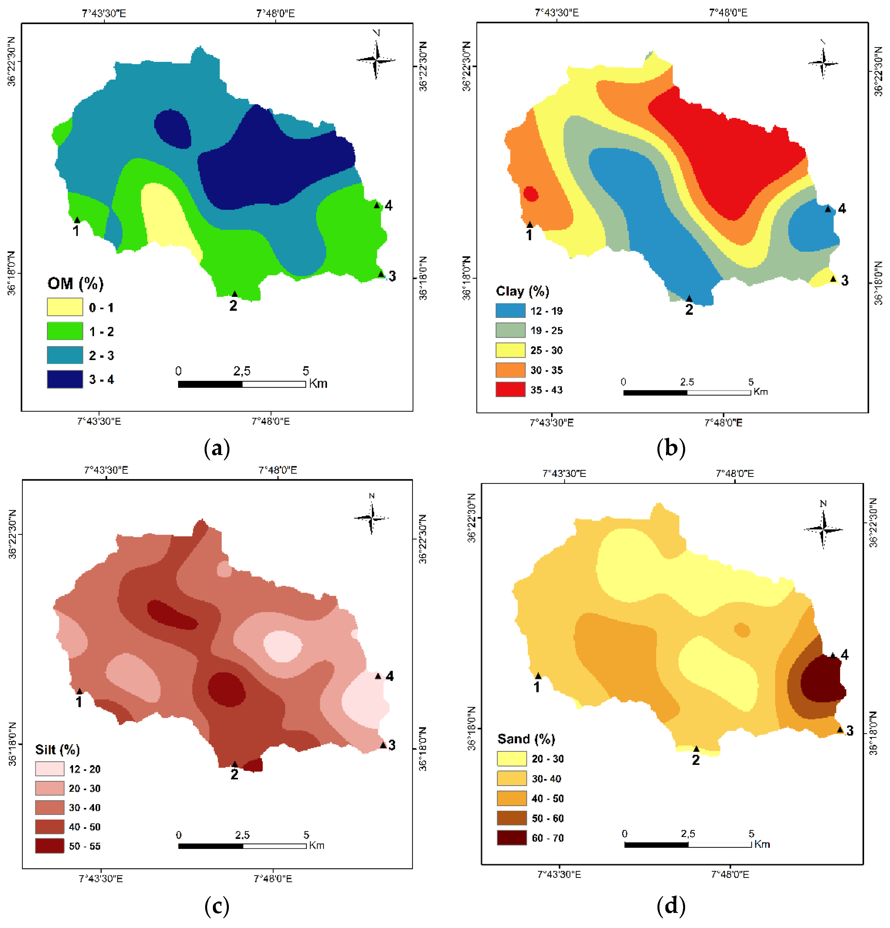
3.5. Geostatistical Analysis

After excluding outliers related to soil attributes and the K parameter, the distribution of the soil datasets was comparable to the normal distribution, indicating that they satisfied the requirement for a stationary or quasi-stationary process in geostatistical analysis. As an example, the K skewness index decreased from 0.773 (before excluding outliers) to 0.557 (without outliers). Soil samples from 132 locations are needed to properly detect anisotropy, which means that it is not feasible to explore directional effects for the dataset related to this study. Since variogram models are assumed to follow the isotropy, only isotropic variogram models are considered for this study.

Soil particle distribution maps for silt, sand, and clay as well as the organic matter, produced by the Kriging interpolation method, are presented in Figure 4.

The maps show that the eastern part of the study area has the least silt content. The majority of this area has a sand content above 30%, while the northeastern portion of the research area has a clay content above 30%. Moreover, the northern part of the basin has more organic matter content than in the south. The average standard errors of the Kriging interpolation maps are 10.96, 9.40, 9.03, and 1.02 regarding the contents of clay, silt, sand, and organic matter, respectively.

The soil erodibility factor spatial distribution map for the complete research region was performed. The ordinary Kriging technique was used to interpolate and estimate the K factor value at unknown places based on the K value of known points (132 sampling points).

A distribution pattern made up of several tiny patches is implied by a narrow effective range [32]. The resulting semivariogram has a nugget/sill ratio (SPD) of 59.46% indicating that the spatial dependence was moderate within a range of 1058 (Figure 5). The remarkable correlation between K parameter predictions and observations confirms the outcome (r = 0.72) and suggests that predicted K values are influenced by neighboring values of observed K over comparatively greater distances.

The ME error values are close to 0 with a value of −2.376537 × 10⁻⁵ and the RMSE error of the K interpolation map is equal to 0.0067, which explains that the prediction values are close to the measured values, thus giving a good prediction. Relative root mean square error (RRMSE) is the root mean squared error normalized by the root mean square value where each residual is scaled against the actual value. It indicates a value of 10.88%, falling between 10% and 20%, which demonstrates the good accuracy and suitability of the K estimation by Kriging.

The Gstat-R programme was used to build the map showing the spatial distribution of the K factor. Figure 6 shows values of the erodibility in the catchment that vary between 0.007 and 0.06. The categorization of the soil’s sensitivity to erosion put out by Wall et al. [46] via the K factor presents 5 classes: very highly susceptible with K > 0.05; highly susceptible: 0.04 < K ≤ 0.05; moderately susceptible: 0.03 < K ≤ 0.04; slightly susceptible: 0.007 < K ≤ 0.03; and very slightly susceptible: K < 0.007.

The lowest values of the K factor were mainly observed in the eastern part of the basin with a slight sensitivity to erosion (0.007 to 0.03) and which occupy 31.29% (25.29 km²) of the basin area. The region is dominated by shrubs and rangelands on mainly moderately sloping surfaces. Its land use is developed on high sandy–clay contents with soil organic matter varying between 1 and 4% (Figure 4). However, the K values in the western region are minor compared with the east, in an area occupied by sparse shrubs and crops. Opposite to the southwest, the northwest area is characterized by high organic matter and clay contents (cropland use). In general, in the soils of the study area, the clay fraction is the key to erodibility as well as the SOM. A higher percentage of SOM was observed in the northeast part of the study area, exceeding 2%. Because the soil has high organic matter content, the aggregates are more stable, which minimizes the susceptibility of the soil to detachment and enhances infiltration. Moreover, higher organic matter minimizes soil loss susceptibility and promotes infiltration [38].

The soils determined to be moderately susceptibility to erosion (0.03–0.04) occupy 53.04% (42.87 km²), and they are spread all over the catchment area, except the mid-south area (Figure 4). The southeast area is characterized by grasslands and sparse shrubs where the slopes are steep. The soil has loam and clay loam textures. Thus, plant root growth and distribution are less important than in the northeast part.

Towards the center and downstream, the agricultural lands are characterized by silt loam, clay loam, and loam soils. There is a significant reduction in soil organic matter, mainly in the south-southwest area. The areas of high organic matter contents are closely related to the management practice of organic amendment addition for cropping. However, tillage practices, planting techniques, and residue management are all responsible for lower organic matter in agriculture. This situation has influenced the soils’ ability to resist erosion, as the occurrence of landslides and gullying has demonstrated.

The high to very high erodibility levels, occupying 12.67 km², are due to the soil texture with low percentages of clay and soil organic matter, and the presence of the slope. The particle size analysis showed the important influence of silt and fine sand fraction content on the erodibility factor [42]. The highly susceptible area to erosion is mainly located in the south of the study basin, which comprises croplands using inappropriate agricultural practices on moderate to steep surfaces, such as plowing in the direction of the slope. In addition, soils developed on Calcic Cambisols tend to present a poor resistance to breakdown and a moderate to low permeability, demonstrating the high sensitivity of the soil against erosion with the lowest percentage of clay aggregates.

Our findings revealed that the spatial distribution of the K factor can be influenced by topographic characteristics of the study basin, different soil use, cropping practices, and physical properties of the topsoil. Considering these soil erosion impacts on soil stability and quality, important measures have to be taken in order to reduce soil degradation and favor safe food production.

4. Conclusions

The regional distribution and impact of the K-factor were examined in this study to provide information on the susceptibility of soil particles to breakup and transport by rainfall and runoff. At the field level, the soil erodibility factor was examined, and the statistical analysis in the Rhirane catchment showed a negative correlation of erodibility with clay and organic matter contents. It was discovered that the presence of silt has a considerable impact on the soil’s susceptibility to erosion. The outcome shows that the K-factor coefficient of variation was 0.36, indicating a modest degree of variability. The Calcic Cambisols which are poorly managed, with land use associated with degraded shrub and grazing fields, showed a soil stability index indicating that this type of soil has a high and severe risk of physical soil degradation.

An exponential function-based framework for mapping soil erodibility is offered by the suggested ordinary Kriging model, in which the semivariogram model was the most effective at explaining the regional distribution of the predicted soil erodibility factor. The calculated soil erodibility factor’s nugget to sill ratio was between 0.25 and 0.75, which is regarded as a moderate level of spatial autocorrelation. The findings showed that soil erodibility ranged from moderate to severe levels, with the greatest estimated soil erodibility factors found in the catchment central and southern regions, and the lowest soil erodibility values found in dispersed areas in the east and west regions.

The results of this study show that in the absence of soil data measurements in the Rhirane basin, the soil erodibility values generated provide an estimate of K-factor values that can be used as guidance for modeling of the potential landscape erosion. In addition, filling knowledge gaps and ensuring implementation of soil conservation practices in the study area is essential to prevent soil loss. Relevant authorities should take long-term and sustainable measures to reduce soil loss and the risks associated with erosion. The spatial distribution of soil erosion in our study can be used to identify the areas that are the most vulnerable to soil erosion. Thus, conservation techniques will be recommended to reduce soil loss in this area. Land use management should focus on agricultural areas and on areas where erosion is high. It is necessary to encourage bicultural practice to ensure security of agricultural products and to manage soil erosion, crop rotation, strip cropping, proper pasture management, contour plowing and planting, and soil conservation practices. It is also essential to promote local reforestation in some areas, which plays an important role against erosion.

References

1. Cassol, E.A.; Silva, T.S.; Eltz, F.L.F.; Levien, R. Soil erodibility under natural rainfall conditions as the K factor of the universal soil loss equation and application of the nomograph fora subtropical Ultisol. Rev. Bras. Cienc. Solo 2018, 42, e0170262. [Google Scholar] [CrossRef] [Green Version]
2. Veazy, A.R.; Bahrami, H.A.; Sadeghi, S.H.R.; Mahdian, M.H. Developing a nomograph for estimating erodibility factor of calcareous soils in North West of Iran. Int. J. Geol. 2011, 5, 93–100. [Google Scholar]
3. Auerswald, K.; Fiener, P.; Martin, W.; Elhaus, D. Use and Misuse of the K factor equation in soil erosion modeling: An alternative equation for determining USLE nomograph soil erodibility values. Catena 2014, 118, 220–225. [Google Scholar] [CrossRef]
4. Tilligkeit, J.K. The Spatial Distribution of K-Factor Values Across a Topo Sequence and a Soil Survey Map Unit. Unpublished. Master’s Thesis, The Faculty of California Polytechnic State University, San Luis Obispo, CA, USA, 2012; p. 43. [Google Scholar]
5. Al Rammahi, A.H.J. Estimation of Soil Erodibility Factor in Rusle Equation for Euphrates River Watershed Using Gis. Int. J. Geomate 2018, 14, 164–169. [Google Scholar] [CrossRef]
6. Liu, M.; Han, G.; Li, X.; Zhang, S.; Zhou, W.; Zhang, Q. Effects of soil properties on K factor in the granite and limestone regions of China. Int. J. Environ. Res. Public Health 2020, 17, 801. [Google Scholar] [CrossRef] [Green Version]
7. Wang, B.; Zheng, F.; Guan, Y. Improved USLE-K factor prediction: A case study on water erosion areas in China. Int. Soil Water Conserv. Res. 2016, 4, 168–176. [Google Scholar] [CrossRef] [Green Version]
8. Islam, M.R.; Jaafar, W.Z.W.; Hin, L.S.; Osman, N.; Karim, M.R. Development of an erosion model for Langat River Basin, Malaysia, adapting GIS and RS in RUSLE. Appl. Water Sci. 2020, 10, 165. [Google Scholar] [CrossRef]
9. Wischmeier, W.H.; Johnson, C.B.; Cross, B.V. A soil erodibility nomograph for farmland and construction sites. JSWC 1971, 26, 183–189. [Google Scholar]
10. Wischmeier, W.H.; Smith, D.D. Predicting Rainfall-Erosion Losses: A Guide to Conservation Planning; U.S. Department of Agriculture, Science and Education Administration: Washington, DC, USA, 1978; p. 537.
11. Wang, G.; Gertner, G.; Liu, X.; Anderson, A. Uncertainty assessment of soil erodibility factor for Revised Universal Soil Loss equation. CATENA 2001, 46, 1–14. [Google Scholar] [CrossRef]
12. Bahrami, H.A.; Vaghei, H.G.; Vaghei, B.G.; Tahmasbipour, N.; Taliey-Tabari, F. A New Method for Determining the Soil Erodibility Factor Based on Fuzzy Systems. JAST 2005, 7, 115–123. [Google Scholar]
13. Vaezi, A.R.; Bahrami, H.A.; Sadeghi, S.H.R.; Mahdian, M.H. Spatial variability of soil erodibility factor (K) of the USLE in North West of Iran. JAST 2010, 12, 241–252. [Google Scholar]
14. Blake, D.; Nyman, P.; Nice, H.; D’Souza, F.M.L.; Kavazos, C.R.J.; Horwitz, P. Assessment of post-wild fire erosion risk and effects on water quality in south-western Australia. IJWF 2020, 29, 240–257. [Google Scholar]
15. Toubal, A.K.; Achite, M.; Ouillon, S.; Dehni, A. Soil erodibility mapping using the RUSLE model to prioritize erosion control in the Wadi Sahouat basin, North-Westof Algeria. Environ. Monit. Assess 2018, 190, 210. [Google Scholar] [CrossRef]
16. Marques, V.; Ceddia, M.; Antunes, M.A.H.; Carvalho, D.; Anache, J.A.A.; Rodrigues, D.B.B.; Oliveira, P.T.S. USLE-K factor method selection for a tropical catchment. Sustainability 2019, 11, 1840. [Google Scholar] [CrossRef] [Green Version]
17. Lin, B.-S.; Chen, C.K.; Thomas, K.; Hsu, C.-K.; Ho, H.-C. Improvement of the K-Factor of USLE and Soil Erosion Estimation in Shihmen Reservoir Watershed. Sustainability 2019, 11, 355. [Google Scholar] [CrossRef] [Green Version]
18. Khanchoul, K. Erosion Hydrique et Transport Solide: Cas de Bassins Versants du Nord-est Algerien, Edition de OmniScriptum; Collection Presses Académiques francophones (PAF): Sarrebruck, Germany, 2015; 312p, ISBN 139783838144719. [Google Scholar]
19. Kriviakine, B.; Kovalenko, E.; Vnouchkov, V. Carte Géologique de Souk Ahras; Editer par Office National de la Géologie; Institut National de la Cartographie: Algiers, Algeria, 1989. [Google Scholar]
20. FAO. Base de Référence Mondiale Pour les Ressources en Sols. Système International de Classification des sols Pour Nommer les Sols el Elaborer les Légendes de Cartes Pédologiques Mises à Jour 2015; Rapport N° 216; FAO: Rome, Italy, 2015. [Google Scholar]
21. FAO. Standard Operating Procedure for Soil Organic Carbon Walkley-Black Method: Titration and Colorimetric Method; FAO: Rome, Italy, 2019; pp. 1–25. [Google Scholar]
22. Pribyl, D.W. A critical review of the conventional SOC to SOM conversion factor. Geoderma 2010, 156, 75–83. [Google Scholar] [CrossRef]
23. Soil Survey Staff. Title 430: USDA-SCS. In National Soils Handbook; U.S. Governmental Printing Office: Washington, DC, USA, 1983. [Google Scholar]
24. Renard, K.G.; Foster, G.R.; Weesies, G.A.; McCool, D.K.; Yoder, D.C. Predicting Soil Erosion by Water: A Guide to Conservation Planning with the Revised Universal Soil Loss Equation (RUSLE). In Agricultural Handbook 703; U.S. Department of Agriculture: Washington, DC, USA, 1997; p. 404. [Google Scholar]
25. Pieri, C. Fertilité des Terres de Savane. Bilan de Trente Ans de Recherche et de Développement Agricoles au Sud du Sahara; Ministère de la Coopération/Cirad: Paris, France, 1989. [Google Scholar]
26. Pieri, C. Fertility of Soils: A Future for Farming in the West-African Savannah; Springer: Berlin/Heidelberg, Germany, 1992. [Google Scholar]
27. Reynolds, W.D.; Drury, C.F.; Yang, X.M.; Fox, C.A.; Tan, C.S.; Zhang, T.Q. Land management effects on the near-surface physical quality of clay loam soils. Soil Tillage Res. 2007, 96, 316–330. [Google Scholar] [CrossRef]
28. Cabezas, A.; Angulo-Martinez, M.; Gonzalez-Sanchis, M.; Jimenez, J.J.; Comin, F.A. Spatial variability in floodplain sedimentation: The use of generalized linear mixed-effects models. Hydrol. Earth Syst. Sci. 2010, 14, 1655–1668. [Google Scholar] [CrossRef] [Green Version]
29. Addis, H.K.; Klik, A.; Strohmeier, S. Spatial variability of selected soil attributes under agricultural land use system in a mountainous watershed, Ethiopia. Int. J. Geosci. 2015, 6, 605–613. [Google Scholar] [CrossRef] [Green Version]
30. Addis, H.K.; Klik, A. Predicting the spatial distribution of soil erodibility factor using USLE nomograph in an agricultural watershed, Ethiopia. ISWCR 2015, 3, 282–290. [Google Scholar] [CrossRef] [Green Version]
31. Cambardella, C.A.; Moorman, T.B.; Novak, J.M.; Parkin, T.B.; Karlen, D.L.; Turco, R.F.; Konopka, A.E. Field-scale variability of soil properties in Central Iowa soils. SSSAJ 1994, 58, 1501–1511. [Google Scholar] [CrossRef]
32. Zhou, Y.; Wang, S.J.; Lu, H.M.; Xie, L.; Xiao, D. Forest soil heterogeneity and soil sampling protocols on limestone outctops: Example from SW China. Acta Carsologica 2010, 39, 115–122. [Google Scholar]
33. Wackernagel, H. Multivariate Geostatistics: An Introduction with Applications; Springer: Berlin/Heidelberg, Germany, 1995. [Google Scholar]
34. Seidel, E.J.; Oliveira, M.S. A classification for a geostatistical index of spatial dependence. Rev. Bras. Cienc. Solo 2016, 40, e0160007. [Google Scholar] [CrossRef] [Green Version]
35. Park, S.J.; Vlek, P.L.G. Environmental correlation of three-dimensional soil spatial variability: A comparison of three adaptive techniques. Geoderma 2022, 109, 117–140. [Google Scholar] [CrossRef]
36. Kannan, K.S.; Manoj, K.; Arumugam, S. Labeling methods for identifying outliers. Int. J. Stat. Syst. 2015, 10, 231–238. [Google Scholar]
37. Wilding, L.P. Spatial Variability: Its Documentation, Accommodation and Implication to Soil Surveys. In Soil Spatial Variability Proceedings of a Workshop of the ISSS and the SSA; Nielsen, D.R., Bouma, J., Eds.; Center Agricultural Pub & Document: Washington, DC, USA, 1985; pp. 166–194. [Google Scholar]
38. Benslama, A.; Khanchoul, K.; Benbrahim, F.; Boubehziz, S.; Chikhi, F.; Navarro-Pedreno, J. Monitoring the Variations of Soil Salinity in a Palm Grove in Southern Algeria. Sustainability 2020, 12, 6117. [Google Scholar] [CrossRef]
39. Ferreira, V.; Panagopoulos, T.; Andrade, R.; Guerrero, C.; Loures, L. Spatial variability of soil properties and soil erodibility in the Alqueva reservoir watershed. Solid Earth 2015, 6, 383–392. [Google Scholar] [CrossRef] [Green Version]
40. Barthes, B.; Roose, E. Aggregate stability as an indicator of soil susceptibility to runoff and erosion; validation at several levels. Catena 2002, 47, 133–149. [Google Scholar] [CrossRef] [Green Version]
41. Perez-Rodriguez, R.; Marques, M.J.; Bienes, R. Spatial variability of the soil erodibility parameters and their relation with the soil map at subgroup level. Sci. Total Environ. 2007, 378, 166–173. [Google Scholar] [CrossRef]
42. Carlos, A.B.; Odette, I.J. Soil erodibility mapping and its correlation with soil properties in Central Chile. Geoderma 2012, 189–190, 116–123. [Google Scholar]
43. Parysow, P.; Wang, G.; Gertner, G.; Anderson, A.B. Spatial uncertainty analysis for mapping soil erodibility based on joint sequential simulation. Catena 2003, 53, 65–78. [Google Scholar] [CrossRef]
44. Huang, T.C.C.; Lo, K.F.A. Effects of land use change on sediment and water yields in Yang Ming Shan National Park Taiwan. Environments 2015, 2, 32–42. [Google Scholar] [CrossRef] [Green Version]
45. Oades, J.M. Soil organic matter and structural stability: Mechanisms and implications for management. Plant Soil 1984, 76, 319–337. [Google Scholar] [CrossRef]
46. Wall, G.J.; Coote, D.R.; Pringle, E.A.; Shelton, I.J. RUSLE-CAN-Équation universelle révisée des pertes de sol pour application au Canada. In Manuel Pour L’évaluation des Pertes de Sol Causées par L’érosion Hydrique au Canada; No de la Contribution AAC2244F; Direction Générale de la Recherche, Agriculture et Agroalimentaire Canada: Sherbrooke, QC, Canada, 2002; 117p. [Google Scholar]
Figure 1. Location map of the Rhirane catchment.
Soilsystems 07 00032 g001
Figure 2. Pictures showing soil erosion in the region of Dahouara: (a) sheet wash and gullies on Chromic Cambisols soil occupied by sparse grassland and shrubs; (b) sheetwash and rills on Calcic Cambisols soils with cultures.
Soilsystems 07 00032 g002
Figure 3. Pictures showing soil analysis in the laboratory: (a) determination of organic carbon; (b) removal of calcium carbonate; and (c) Robinson’s pipette technique.
Soilsystems 07 00032 g003
Figure 4. Maps of soil properties and organic matter distribution: (a) organic matter; (b) clay; (c) silt; (d) sand. Research locations: 1—El Koukez Hills, 2—Ras el Arous Hills, 3—El-Mekmen Hills, and 4—El Guelala hills.
Soilsystems 07 00032 g004
Figure 5. Semivariogram of soil erodibility (K).
Soilsystems 07 00032 g005
Figure 6. Spatial variability of soil erodibility factor on the exanimated area at Rhirane catchment. Research locations: 1-El Koukez Hills, 2-Ras el Arous Hills, 3 El-Mekmen Hills, and 4-El Guelala hills.
Soilsystems 07 00032 g006