Methane and Nitrous Oxide Emission Fluxes Along Water Level Gradients in Littoral Zones of Constructed Surface Water Bodies in a Rewetted Extracted Peatland in Sweden

Abstract

Rewetted extracted peatlands are sensitive ecosystems and they can act as greenhouse gas (GHG) sinks or sources due to changes in hydrology, vegetation, and weather conditions. However, studies on GHG emissions from extracted peatlands after rewetting are limited. Methane (CH₄) and nitrous oxide (N₂O) emission fluxes were determined using the opaque closed chamber method along water level gradients from littoral zones to the open water body of constructed shallow lakes with different vegetation zones in a nutrient-rich rewetted extracted peatland in Sweden. Vegetation communities and their position relative to water level, together with short-term water level fluctuations, such as inundation events and seasonal droughts, and temperature had a significant impact on CH₄ emissions fluxes. During “normal” and “dry” conditions and high soil temperatures, CH₄ emissions were highest from Carex spp.-Typha latifolia L. communities. During inundation events with water levels > 30 cm, sites with flooded Graminoids-Scirpus spp.-Carex spp. emitted most CH₄. Methane emissions from the water body of the constructed shallow lakes were low during all water level conditions and over the temperature ranges observed. Nitrous oxide emissions contributed little to the emission fluxes from the soil-plant-water systems to the atmosphere, and they were only detectable from the sites with Graminoids. In terms of management, the construction of shallow lakes showed great potential for lowering GHG emission fluxes from nutrient rich peatlands after peat extraction, even though the vegetated shore emitted some N₂O and CH₄.

1. Introduction

Boreal and subarctic peatlands cover considerable areas in the northern hemisphere [1]. Peat extraction for horticultural purposes and energy production has a long tradition in Northern Europe and can typically be performed on a peatland for up to 40 years [2].

According to the Swedish law, remediation of the site is required after the peat has been extracted. Productive forestry and agriculture are two possible after-uses but for those measures drainage is required, which would cause decomposition of the remaining peat and thus continuing emissions of carbon dioxide (CO₂). For nutrient-rich sites, nitrous oxide (N₂O) can also be a significant source of greenhouse gases (GHG) [3].

Another after-use alternative is rewetting [4,5,6], which has been encouraged as a land use management practice in order to reduce GHG emissions and thus mitigate climate change due to carbon (C) sequestration [7,8,9]. In addition, rewetting can decrease water pollution and stop subsidence, the irreversible structural collapse of the peat body [10]. Rewetting can also create habitat for migratory and breeding birds [11] and prevent loss of biodiversity [12]. Rewetting is thus the first step in peatland restoration aiming to change the hydrological conditions to accomplish functioning wetlands [13]. “Thriving wetlands” is one of Sweden’s 16 environmental quality objectives and it requires damaged wetlands, such as bogs and fens, to be restored to preserve their valuable ecosystem services. Starting more than 20 years ago, some Swedish peatlands drained for peat extraction have been rewetted [14,15,16,17] and functioning wetland ecosystems with stable hydrology and characteristic peatland vegetation have been established. However, rewetted peatlands are sensitive ecosystems and they can act as GHG sinks or sources due to small changes in hydrology, vegetation, and weather conditions [18].

The desired restoration goal with rewetting is re-establishment of the peatland’s ecosystem functions [19]. How successfully this goal can be achieved depends on the existing environmental conditions, such as the used extraction method, the residual peat depth and peat type, the topography of the remaining peat surface together with its landscape situation, and the availability and quality of water resources [6,20,21].

Due to the different initial situations after peat extraction, a systematic overview of GHG exchange from such areas is lacking [6] and therefore it is difficult to predict how rewetting affects the GHG dynamics in a peatland [22]. Although default emission factors for CO₂, methane (CH₄), and N₂O from peatlands managed for extraction are to be found in the IPCC Wetlands Supplement [9], emission factors after rewetting are only given for the categories ‘nutrient status’ and ‘climate zone’ but not explicitly for ‘land uses’, such as rewetting after peat extraction. Thus, sites with different land uses before rewetting (e.g., agriculture, forestry and extraction) are grouped together and therefore lacking individual emission factors.

There are many studies on GHG emissions from peatlands and riparian wetlands formerly used for agriculture (e.g., [23,24,25]), whereas studies on GHG emissions from extracted peatlands after rewetting are limited. In general, peatland rewetting decreases emissions of CO₂ and N₂O, while CH₄ emissions may increase (e.g., [26,27,28,29]). However, it is also important to consider the transition time for emissions of a certain gas after rewetting [30]. Pointing out that a peatland’s return to a C sink is highly site-specific, CO₂ emissions may be reduced in this period, but the recovery of the C sink function may take decades [18]. In the presence of fresh organic material, temporarily or persistently high CH₄ fluxes over decades after rewetting have been found [18,31,32].

Furthermore, the magnitude of GHG fluxes from peatlands depends on various site parameters. For example, Couwenberg et al. [33] concluded that mean annual water level and vegetation are good proxies for GHG fluxes from peatlands in general. Vegetation not only reflects long-term water levels, but also directly affects GHG emissions due to assimilate supply (CO₂) and CH₄ transport to the atmosphere via the aerenchymatous system of the plants [33,34,35].

Studies on GHG emission fluxes from rewetted extracted peatlands have been followed up in different time periods after rewetting [15,22,34,36,37,38,39,40,41]. However, these results have to be complemented with information on how GHG fluxes change over space and time. More data are needed on GHG emissions from extracted peatlands over longer periods after rewetting [42,43] and from corresponding studies about constructed water bodies in general (e.g., shallow lakes), surrounded by vegetated littoral zones, which have been identified as high CH₄ emitters [44,45], but also as low CH₄ emitters compared with open water [46].

The overall aim of this study was to investigate and quantify CH₄ and N₂O emission fluxes along water level gradients (transects) from the rather dry vegetated shore, over the littoral zones to the open water without vegetation of constructed shallow lakes with wetland and non-wetland type vegetation zones in a terminated extracted peatland after rewetting. It was further determined how these fluxes change following short-term inundation events and seasonal droughts.

Monitoring was conducted to obtain multi-year data on CH₄ and N₂O fluxes but not to prepare annual GHG budgets. The study was carried out in sub-boreal central Sweden and was part of the long-term project “Restoration of terminated peat cuttings by rewetting” [15,16,17,21,47].

2. Materials and Methods

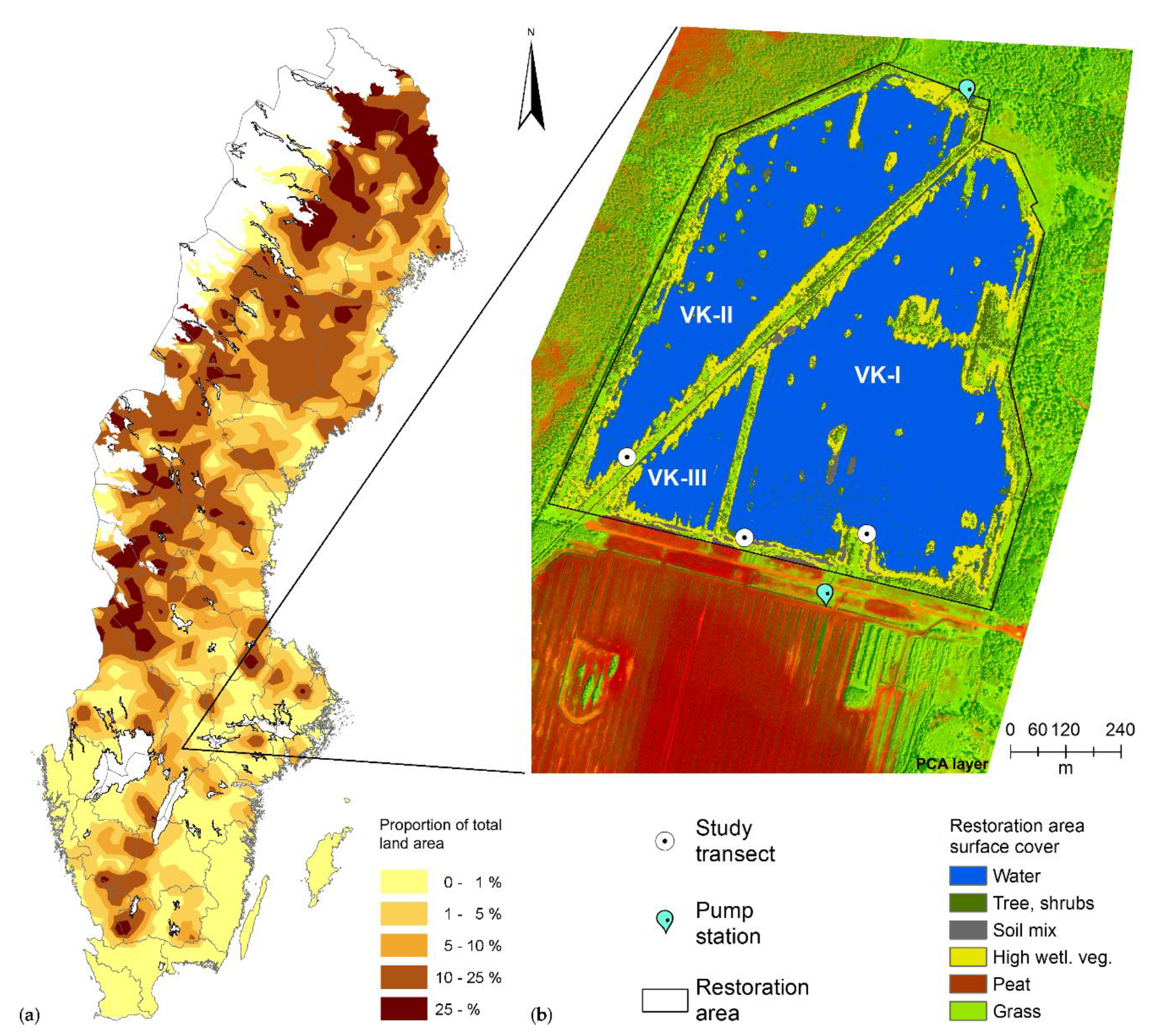
2.1. Site Description

The Västkärr wetland is a rewetted peat extraction site (Figure S1) in the lagg area of Skagerhultamossen, one of south-central Sweden’s largest bogs (59°06′ N, 14°45′ E; 65 m above sea level). It is situated in Lekebergs municipality, 50 km south-west of the city of Örebro (Figure 1a). The climate is semi-humid and maritime [48], with mean annual temperature of 5.7 °C, mean annual precipitation of 690 mm (1961–1990; [49]) and a growing season of 200 days (temperature >5 °C for four consecutive days; [50]). During the years since rewetting (1999–2013), precipitation has been 9% higher and temperature has been 0.7 °C warmer (4 × 4 km gridded data; [51]) than the regional 30-year average 1961–1990.

Prior to peat extraction, the lagg area of the bog had been drained for hay production and cereal cultivation since the 19th century. In the 1970s, intensive drainage for potato cultivation took place at that area (Figure 1b). Milled peat extraction for energy use started in 1987 and continued until 1997. Mean annual volume of extracted peat was 120,000 m³ on 195 ha. At the time just before rewetting, the bottom of the prospective constructed lakes consisted of 0.1–0.2 m highly decomposed fen peat (H 8 to H 10 [52]; bulk density of 0.2–0.3 g cm⁻³, pH 5–6 and C/N ratio 21) on postglacial clay. Further site descriptions can be found in [16,17]. The northern part of the previous peat extraction area in Västkärr peatland (Figure 1b) was prepared for rewetting in 1998, with water storage starting in 1999. Rewetting established three shallow lakes (VK I, VK II, VK III) with a total surface area of 80 ha and with mean water depth of approximately 1 m on the central parts of the water bodies. These shallow lakes, which have many small constructed peaty islands, are valuable habitats for common and rare migration bird species.

Peat extraction is still ongoing in the middle part of the Västkärr peatland, south of the rewetted area (Figure 1b). Beside the surface water and precipitation water supply, drainage water is continuously being pumped from the active peat extraction to the rewetted site.

The dominant mesotrophic and eutrophic wetland plant species in Västkärr are Carex spp., Phragmites australis (Cav.) Trin. ex Steud., Scirpus spp. and Typha latifolia L. Other helophytes and hydrophytes such as Alisma plantago-aquatica L., Butomus umbellatus L., Hydrocharis morsus-ranae L., Juncus spp., Lythrum salicaria L. and Sparganium spp. also occur. Lemna minor L. is ubiquitous between late June and October. Graminoids such as Calamagrostis canescens (Weber ex F.H. Wigg.) Roth, Poa trivialis L. and Phalaris arundinacea L. dominate the dryer parts of the shore and the constructed ridges between the lakes. Vegetation composition has changed somewhat over time since rewetting in terms of cover values [47], due to intense water level fluctuations, both within and between the years.

2.2. Field Sampling and Measurements

For the purposes of measurements, wooden boardwalks were installed on the southern shores of the constructed lakes VK I and VK II (Figure 1b), with longitudinal directions towards the lake limnetic zones to prevent disturbance to the peat by trampling and to facilitate measurements in water. The mean residual peat depth was 120 cm along the boardwalk at VK II and 40–90 cm along the boardwalks at VK I.

Soil sampling to determine soil characteristics for valuable background information, such as total contents of several elements, bulk density, and pH, was carried out from the two peat horizons above the underlying clay soil on the non-inundated shore zone at VK II. Additional peat samples were taken from the lake bottom at all three sites. Degree of peat decomposition has been determined in the field [52]. Total C and total nitrogen (N) from peat samples were quantified by dry combustion in a C/N analyser (CN2000, Leco, USA) according to [54,55]. Surface water samples were collected from the three study sites and from a ditch at the pumping station 4 to 6 times per year from 2009 to 2013 for determination of pH, electrical conductivity, dissolved organic carbon (DOC), and total C according to [56,57,58].

Methane and N₂O emission flux measurements were performed on 15 occasions during daytime in the snow-free period (April to October) from 2009 to 2014. Twenty-four GHG flux measurement positions (frames or floating chambers) were established along three transects (Figure 1b and Figure S2), each approximately 20 m long, in different types of vegetation zones and on the (vegetation-free) water of the lake. In these zones, vegetation communities of homogenous and mixed stands (due to succession and water table changes) were identified and grouped together: Graminoids in the typically non-inundated shore zones, Graminoids-Scirpus spp.-Carex spp. in the typically non-inundated but temporarily inundated zone of the littoral and Carex spp.-Typha latifolia in the reed bed of the littoral with typical water depths around 0.3 m. No bare peat sites were monitored. These water level conditions were taken as ‘normal’ and they changed to ‘dry’ or ‘inundated’ conditions from time to time, meaning that the whole transect was lying above or below the water level, respectively. Thus, it was expected to investigate how GHG emissions from those vegetation reacted in ‘normal’, dry and inundated conditions.

When seasonally flooded, floating chambers for GHG measurements were used almost exclusively. When the water level became very low, frames were used instead of floating chambers. The frames in the littoral zone were adapted in height to the plant development and to water level. Thus, young Typha latifolia plants, which fitted in the chamber without bending, were measured in spring and early summer. Since Typha latifolia could reach heights of up to 2.5 m, GHG flux measurements within the community were performed without including plants in the chamber between late June and late October. Due to technical circumstances, it was not possible to measure in the Typha latifolia stands with flexible chambers, such as in [35].

On every GHG flux measurement occasion and adjacent to each measurement position, soil or water temperature at 10 cm depth was determined by means of an electronic thermometer. Water level was recorded manually using a meter stick. Plant species and plant cover were described at each measurement position.

2.3. Greenhouse Gas (GHG) Flux Determination

2.3.1. Chamber Sampling and Measurement of GHG Concentration

The CH₄ and N₂O emission flux measurements were carried out using the opaque closed chamber method [59,60]. For gas sampling at the vegetated shore, permanent annular PVC frames (inner base diameter 18.7 cm) were installed at each GHG flux measurement position. Due to water table changes and vegetation succession, the number of GHG flux measurement positions were not constant over time but covered 1…13 (Graminoids), 1…8 (Graminoids-Scirpus spp.-Carex spp.), 0…12 Carex spp.-Typha latifolia and 0…4 (water) positions per sampling occasion, respectively. To avoid lateral gas exchange in the soil, insertion depth of the frames varied due to different soil water conditions [61,62].

For gas flux measurements, a non-steady-state flow-through opaque respiration chamber was attached to the frame and sealed with a rubber gasket. The chamber was made of PVC with 18.7 cm inner base diameter and 16 cm height and had an effective chamber air volume of 4.3 ℓ. Air samples were taken in crossflow through the chamber headspace with polysiloxane tubing. Effective frame air volume was determined on each GHG measurement occasion, with consideration of uneven soil surfaces and plants, to obtain the individual headspace air volume (sum of chamber and effective frame air volumes). A chamber installed in the centre of a life buoy (i.e., floating chamber) with similar dimensions and an effective headspace air volume of 3.0 ℓ was used for GHG measurements on open water.

For measurements of CH₄ and N₂O volume concentrations (y_gas) in headspace air, 20 mℓ air samples were collected in glass vials with 20 mm/3.0 mm butyl-PTFE septum in an aluminium seal cap (Scantec Nordic, Sweden) at 10, 20, 30, 40, and 50 min (2009–2010), 10, 20, 30, and 40 min (May 2012), 10, 20, and 30 min (June 2012 to October 2013) or 1, 11, 21, 31, and 41 min (2014) after chamber closure, respectively. Air was circulated with an external membrane pump (volume flow rate 0.4 ℓ min⁻¹) between the chamber and the vial over 20 s (seven air exchanges in the vial). The CH₄ and N₂O samples were stored in the dark at room temperature and were analysed between one day and two weeks after sampling with a gas chromatograph (GC) (Clarus 500, Perkin Elmer, MA, USA) equipped with a flame ionisation detector, an electron capture detector and an automatic vial headspace injector (Turbo Matrix 110, Perkin Elmer, USA). Obviously leaky vials (vials with fissure or neck breakage, damaged crimp cap or creased internal septum surface) were discarded.

Methane standards of 2, 10, 20, and 350 ppmn and N₂O standards of 0.3, 1.7, and 4.7 ppmn (AGA, Sweden) were used for calibration. Calibration functions were established for ranges from 2 ppmn to 20 ppmn or from 2 ppmn to 350 ppmn CH₄, depending on the range found for the sample set on a measurement occasion. The standards’ certified mixture compositions were given in amount fraction (ppmn), however, the volume concentration (ppmv) was used in the present study (1 ppmn ≙ 1 ppmv, from Dalton’s law) [63,64,65].

All GC data were reprocessed with an improved peak integration method in the GC’s software in 2016/2017. The 95% confidence intervals (Δy_gas) of the obtained concentration values (y_gas) are ±4.0% of the CH₄ concentration at y_gas ≈ 2 ppmv CH₄, ±0.13 ppmv N₂O for the year 2009′s analyses and ±0.035 ppmv N₂O for the years 2010…2014′s analyses at y_gas ≈ 0.3 ppmv N₂O, respectively.

2.3.2. Flux Estimation and Evaluation

The CH₄ and N₂O fluxes were estimated according to

F = f’(t₀) · p · V / (A · R · T),

(1)

where F is the molar flux to the atmosphere. The first functional derivative f’(t₀) at the moment of chamber closure t₀ is estimated from the regression function

f(t) = y_gas(t)

(2)

of the change in volume concentration y_gas in headspace air over time t and given as concentration per unit time; p is the atmospheric pressure, V the headspace air volume, A the chamber base area, R the molar gas constant, and T the sample air temperature.

Linear and quadratic regressions (cf. [66,67]) were estimated. As some measured series of headspace CH₄ or N₂O concentrations consisted of three valid values, only linear regression was used to estimate CH₄ and N₂O fluxes for these series (cf. [59,68,69]). All regression functions had to fulfil some empirical plausibility criteria to be accepted as valid for flux estimation [15]. For each y_gas time series, the valid regression with the least residual standard deviation (cf. [66]) was used to estimate the flux.

If the range of y_gas during chamber closure was less than $\sqrt{2}$ times larger than the 95% confidence interval (Δy_gas) of the mean concentration (thus, the range was within the analysis’ repeatability; [70]), the resulting flux was classified as non-detectable. If the range of y_gas was larger than that and if the y_gas time series failed the von Neumann trend test ([70]; P ≥ 95%; test only applicable for series with n ≥ 4 values), the resulting flux value was rejected as estimated from a headspace concentration change without a significant trend, likely to result from disturbed y_gas time series measurements.

Disturbances in the flux estimation obviously due to ebullition (non-diffusive release of gas) were detected for any single CH₄ concentration time series by testing some further plausibility criteria [15]. If a disturbance by ebullition in the flux estimation was plausible, the related CH₄ flux estimate was discarded. Those disturbances may otherwise lead to both over- and underestimations of the real flux. CH₄ emissions via ebullition were not generally excluded from the resulting flux data set, but only those concentration time series that were not suitable to estimate a flux from a regression function’s slope. Examples for regressions of CH₄ concentration time series with or without disturbances by ebullition are given in Figure S3.

2.3.3. GHG Flux Detection Limits

The flux detection limit (F_DL) was estimated in a simple approach [15,35,66,71,72]: It was assumed that a concentration change in the chamber headspace air had to exceed the analysis’ repeatability to be detectable. Therefore, the GC’s repeatability coefficient $\sqrt{2}$ Δy_gas for CH₄ and N₂O, respectively, was set as the concentration change between the first and last measurement of a presumed headspace air determination. F_DL was calculated according to Equation (1), setting the slope of this presumed concentration change as f’(t₀) and using the effective V of each flux measurement position.

2.4. Statistical Analyses of CH₄ Flux

A linear mixed effects analysis (cf. [73,74,75]) was performed to investigate how CH₄ fluxes were affected by different environmental conditions. The analysis was carried out using the packages lme4 and car in R x64 3.2.2 [76,77,78,79]. The linear mixed effects models built in this analysis combined the flux to the atmosphere as the response variable with observations of some adjacent environmental conditions (e.g., temperature, vegetation community, water level) as independent variables that were set as fixed or random effects. Herewith, soil and water temperatures were pooled in a single data set. To identify the best fitting model, P-values and Akaike’s Information Criterion (AIC) were obtained by likelihood ratio tests comparing a model with the effect in question against the respective model without the effect in question (cf. [74,75]). The models were also checked and compared for good approaches to homoscedasticity and normality. The natural logarithm of the flux was used as response variable to meet normality and homoscedasticity requirements and to improve the significance of the linear mixed effects models obtained. To permit the flux values to be transformed into logarithms, non-detectable CH₄ fluxes were replaced with a value of half the CH₄ flux detection limit F_DL [72] to prevent (non-significant) negative flux values.

3. Results and Discussions

3.1. Soil Physical and Chemical Conditions

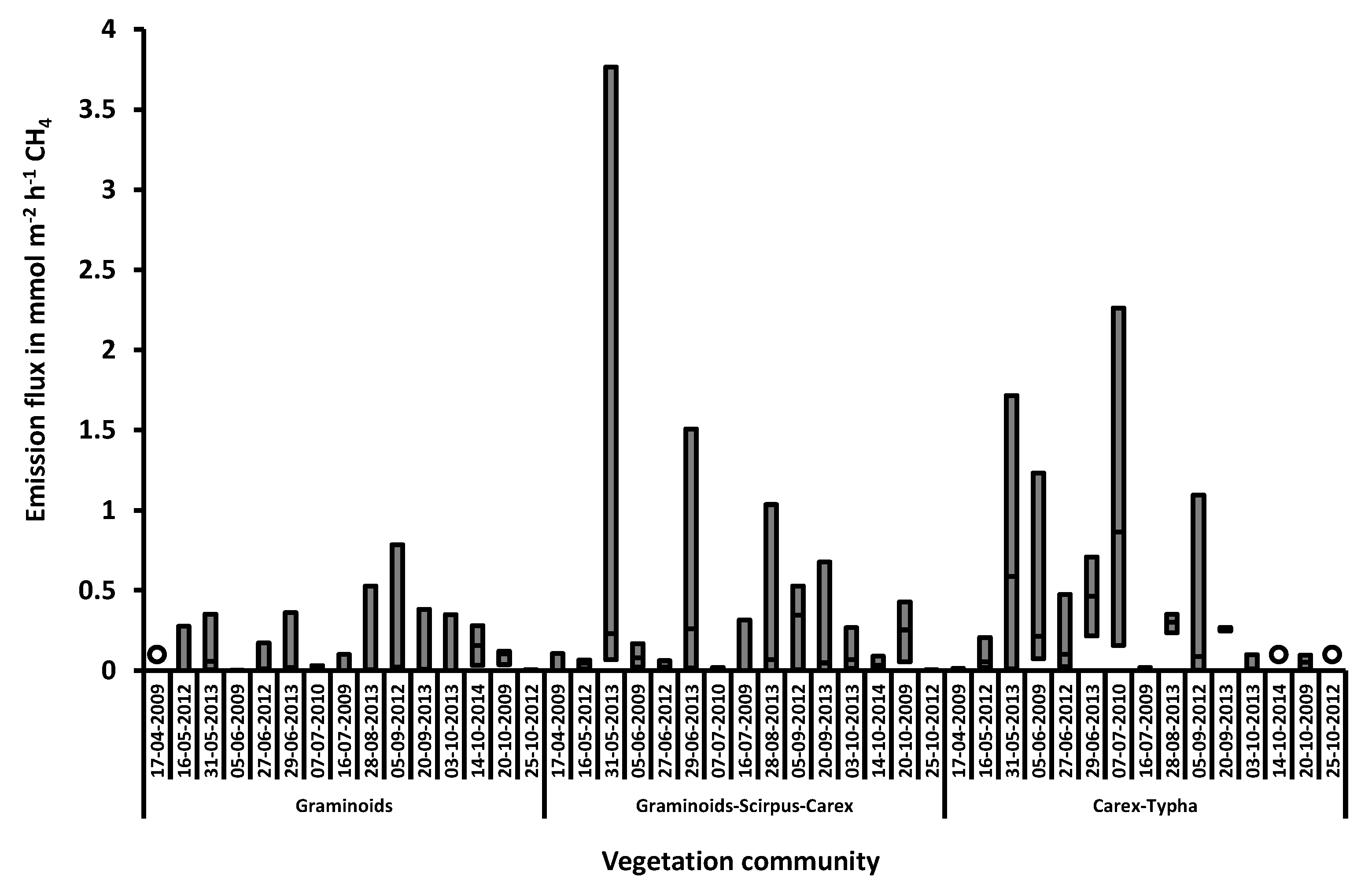
The main peat type at all three transects was highly decomposed fen peat with degree of peat decomposition H 8–10 in the uppermost horizon and H 5 in the subjacent horizon. Mean values for peat soil properties are summarized in

Table 1. Soil properties in different horizons at the study transects (see Figure 1); elements in aqua regia digestion; n.d. = not determined.

Soil Property	Lake VK II			Lake VK I		Adjacent Peat Extraction Site
				(west)	(east)
	0–22 cm	23–35 cm	Lake Bottom 5–22 cm	Lake Bottom 0–10 cm	Lake Bottom 0–12 cm	Loose Peat
Median C/N ratio (min.-max.)	20.1 (19.7–20.3)	22.5 (21.6–23.0)	21.4	24.1	22.2	n.d.; 96% loss on ignition
Median bulk density in g cm−3 (min.-max.)	0.36 (0.27–0.42)	0.17 (0.17–0.23)	n.d.	n.d.	n.d.	n.d.
pH in water	5.0	5.6	5.9	5.4	5.3	5.2
Al in g kg−1	5.5	2.2	13.4	6.6	9.7	3.2
Ca in g kg−1	12.1	11.8	8.8	13.9	12.5	3.8
Fe in g kg−1	14.9	4.7	18.9	10.7	10.4	2.2
K in g kg−1	0.27	0.09	3.05	0.42	0.62	0.12
Mg in g kg−1	0.64	0.50	4.48	1.14	1.20	0.25
Mn in g kg−1	0.83	0.51	0.61	0.49	0.34	0.08
Na in g kg−1	0.08	0.07	0.27	0.12	0.10	0.06
P in g kg−1	0.68	0.31	0.41	0.55	0.51	0.25
S in g kg−1	3.5	3.2	2.2	5.1	5.2	2.8

.

Surface water conditions were characterised by pH 6,6 (median), electrical conductivity 89 μS cm⁻¹ (median), DOC concentration of 39 mg ℓ⁻¹ and total C concentration of 41 mg ℓ⁻¹ (median values 2009). More environmental data over the entire period from before rewetting in 1997 until 2013 can be found in [17]. Mean values for soil and water temperature as well as water level categories on each measurement occasion are summarised in

Table 2. Mean soil and water temperatures in °C at 10 cm depth and water level categories at the study transects; i = inundated; ni = non-inundated; i&ni = partially inundated; n.d. = not determined.

Measurement Occasion (month-year)	Vegetation Community						Water
	Graminoids		Graminoids-Scirpus-Carex		Carex-Typha
04-2009	7.1	i	4.2	i&ni	10.9	i	12.3
06-2009	10.2	ni	10.0	ni	10.4	i&ni	12.5
07-2009	21.6	i	20.3	i	21.0	i	21.5
10-2009	5.0	i&ni	5.0	i	5.2	i	5.1
07-2010	17.0	ni	15.1	ni	16.8	ni	23.9
05-2012	10.3	i&ni	12.1	i	16.7	i	17.3
06-2012	14.3	i&ni	13.4	i&ni	18.3	i	18.0
09-2012	13.8	i&ni	13.6	i&ni	14.3	i	14.3
10-2012	5.7	i	5.8	i	n.d.	i	5.7
05-2013	15.2	i&ni	16.1	i&ni	22.0	i	21.5
06-2013	15.3	i&ni	14.6	i&ni	16.9	i	15.5
08-2013	13.0	i&ni	12.8	i&ni	12.9	i	11.2
09-2013	10.2	ni	10.1	i&ni	9.2	i	8.0
10-2013	6.0	ni	5.8	i&ni	4.0	i&ni	2.7
10-2014	7.7	i&ni	7.6	i	7.0	i	7.4

.

3.2. Methane Fluxes

From 214 successful CH₄ flux estimations, 178 flux values were above and 36 values were below flux detection limit. A further 38 flux values were discarded because of obviously disturbed headspace concentration time series measurements. The 95-percentile of all 214 CH₄ emissions flux values at the VK transects was found to be 778 µmol m⁻² h⁻¹. We are aware that the data set is small and that we might have got a non-representative data set for the CH₄ emission dynamics. An overview about CH₄ emission fluxes in the littoral zone is given in Figure 2.

3.2.1. Linear Mixed Effects Analysis

Due to the used vial sampling technique with high uncertainties in a single flux measurement and inhomogeneous field data sets, an averaging of the data has been excluded. Thus, a linear mixed effects model has been used as a statistical analysis to aggregate data and to obtain a rough tendency for GHG emissions from vegetation in relation to temperature and moisture. Raw data and modelled data are shown in Figure 3. Here, high uncertainties in the raw data distribution are visible. The model’s coefficients and their uncertainties are to be found in

Table 3. Parameters of the linear mixed effects model for CH₄ fluxes to the atmosphere from the vegetation communities. Significant fixed effects and coefficients in bold. Reference level for vegetation community: graminoids; reference level for water level category: non-inundated. T_i = soil/water temperature; vc = vegetation community; wlc = water level category; i = inundated; ni = non-inundated; est. = estimate; SE = standard error; t = t value. Random effect’s intercept b₅ = ±0.5 (standard deviation SD = 0.74) adapting for measurement positions on (+) or between (−) plant individuals.

Coefficient		a1= aj			b1			b2			b3			b4			Σ bj
Fixed Effect		Ti			vc			vc × wlc			wlc			intercept
Pr (> chi-square)		1.3 × 10−4			4.9 × 10−11			1.4 × 10−5			4.2 × 10−2
vc	wlc	est.	SE	t	est.	SE	t	est.	SE	t	est.	SE	t	est.	SE	t
Water without vegetation	i	0.11	0.029	3.8	−1.4	0.76	−1.8				1.9	0.50	3.9	0.1	0.69	0.2	0.7
Carex-Typha	ni	0.11	0.029	3.8	3.9	0.55	7.0							0.1	0.69	0.2	4.0
Carex-Typha	i	0.11	0.029	3.8				−3.5	0.76	−4.7	1.9	0.50	3.9	0.1	0.69	0.2	2.4
Graminoids-Scirpus-Carex	ni	0.11	0.029	3.8	2.0	0.39	5.3							0.1	0.69	0.2	2.2
Graminoids-Scirpus-Carex	i	0.11	0.029	3.8				−1.0	0.69	−1.5	1.9	0.50	3.9	0.1	0.69	0.2	3.1
Graminoids	ni	0.11	0.029	3.8										0.1	0.69	0.2	0.1
Graminoids	i	0.11	0.029	3.8							1.9	0.50	3.9	0.1	0.69	0.2	2.0

.

Vegetation community and water level category (with interaction term) and soil/water temperature were obtained as significant fixed effects in the linear mixed effects analysis of the relationship between CH₄ fluxes and some adjacent environmental conditions. A random effect representing measurement positions between the plant individuals significantly improved the model.

There was a significant linear relationship between soil/water temperature and the natural logarithm of the CH₄ fluxes as a response variable in the model. Thus, the model estimated the fluxes to the atmosphere from a vegetation community at a given soil/water temperature as

F_i = e^{(aj · |Ti| + bj)},

(3)

where F_i is the flux to the atmosphere in µmol m⁻² h⁻¹ at soil/water temperature T_i in °C at a flux measurement i. The constants a_j and b_j were coefficients of the model and dependent on the adjacent environmental conditions j that were used as fixed effects (Table 3). The constant a_j may be expressed as

a_j = ln(TS₁₀)/10,

(4)

where TS₁₀ is a soil or water temperature sensitivity coefficient, e.g., the factor of increase of CH₄ production rate with 10 °C temperature increase, that is mathematically analogous to the temperature coefficient Q₁₀ in the van ’t Hoff reaction-rate-temperature rule [80]. Therefore

TS₁₀ = (F_i / F₀)^{10 K / (T_i − T₀)},

(5)

where F_i and F₀ are the fluxes at soil/water temperatures T_i and T₀ = 0 °C.

Visual inspection of the residual plot revealed a slight deviation from homoscedasticity for the CH₄ model due to flux estimates below the detection limit. The approach to normality was good. Although all fixed effects were significant, many regression coefficients were not (Table 3).

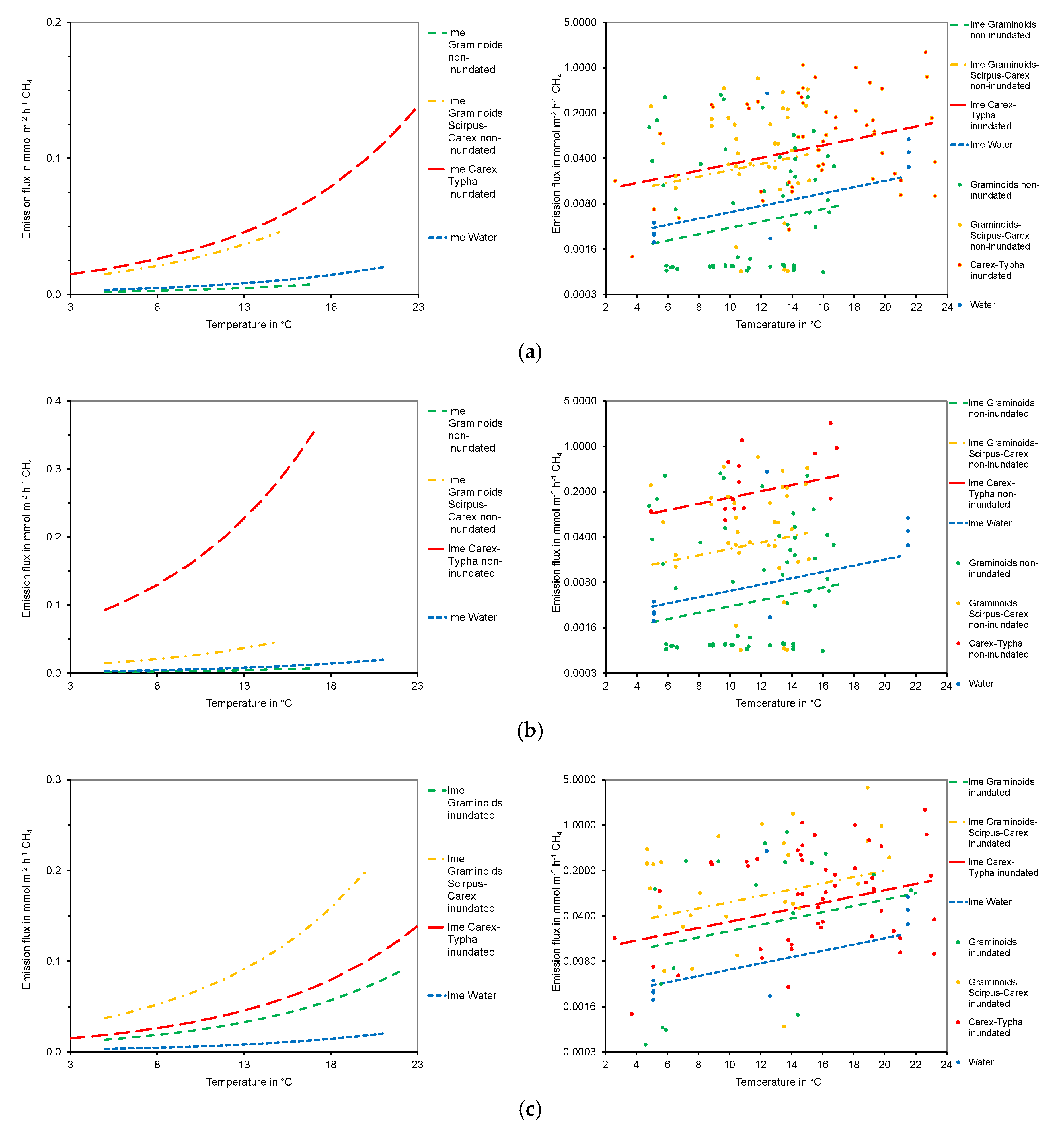
3.2.2. The Model Outcome: Influence of Water Level, Vegetation Community, and Soil Temperature on Methane Fluxes

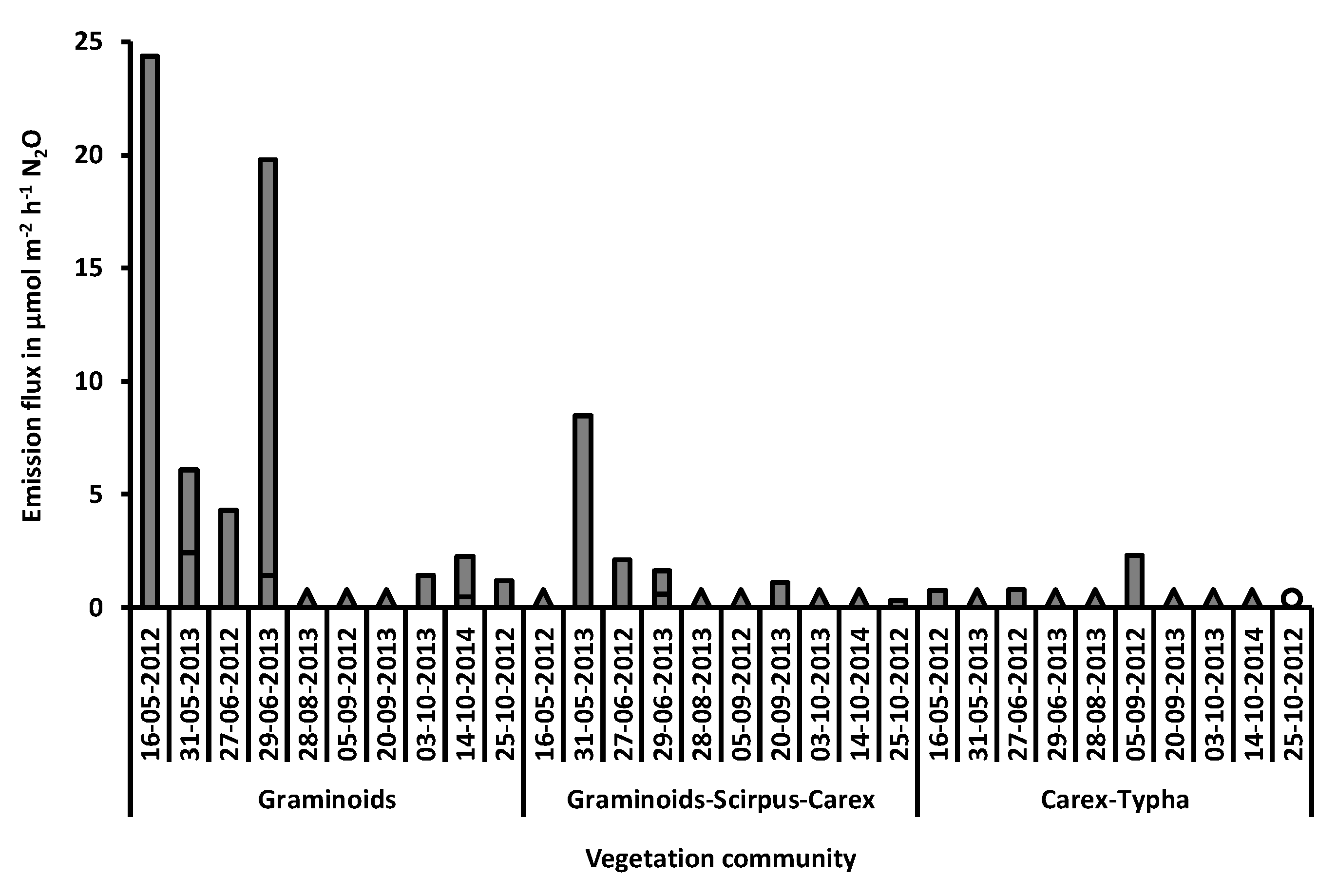
A combination of wetland plant cover and high water level, but also non-inundation and high soil temperature, enhanced CH₄ emissions. This is in line with other studies for rewetted fens (e.g., [41]), shallow lakes [81], and rewetted peat extraction sites [45]. The higher CH₄ fluxes observed with increasing temperature for the Carex spp.-Typha latifolia community were associated with a steep slope in the linear mixed model function (Figure 3a,b). This fact may be explained by the seasonal dynamics of microbial activity and thus, faster CH₄ production rates [82], and by an active plant growth forcing aerenchymatous gas transport [83,84], meaning that CH₄ oxidation can be avoided because the pathway through the upper aerobic peat horizons is bypassed [35]. As Typha latifolia stands could not be measured with flexible chambers, such as in [35], we are aware that we may have underestimated the CH₄ emissions, especially those from the aerenchymatous gas transport, even though measurement positions between the plant individuals are respected in a model’s random effect. The CH₄ emissions from the Carex spp.-Typha latifolia communities in the late vegetation season during all study years under ‘normal’ and ‘inundated’ conditions are far below from the reported data in [85] that included aerenchymatous gas transport.

The estimate of soil temperature sensitivity coefficient TS₁₀ for CH₄ fluxes to the atmosphere based on the linear mixed effects models was uniformly TS₁₀ = 3.0 for the different vegetation communities. Thus, the model indicated that the CH₄ fluxes from the Graminoids but also from the Graminoids-Scirpus spp.-Carex spp. community had the same relative sensitivity to warmer temperatures as those from the Carex spp.-Typha latifolia community and the water. However, the increase in CH₄ emission fluxes was larger for the Carex spp.-Typha latifolia community than for the Graminoids and the Graminoids-Scirpus spp.-Carex spp. communities during ‘normal’ and ‘dry’ conditions. Higher soil temperatures also stimulate CH₄ production [86] and thus CH₄ emissions can be increased [87]. Furthermore, if the roots are still in contact with CH₄ depots in the anaerobic peat horizons, the plant-mediated CH₄ flux to the atmosphere is still active [83] even when the uppermost peat horizon is aerated (Figure 3b). Compared to ‘dry’ conditions, during inundation the CH₄ emission fluxes from Carex spp.-Typha latifolia were reduced (Figure 3c). The CH₄ fluxes from Graminoids might be relatively less affected by a temperature increase during ‘normal’ and ‘dry’ conditions, which was seen in a low CH₄ emission level and a negligible slope (Figure 3a,b). The same pattern turned out to be the case for emission fluxes from the water body (Figure 3).

However, there were exceptions to the temperature pattern (Figure 3c): under inundated conditions, sites with Graminoids started to emit more CH₄ with increasing temperature compared to ‘normal’ and ‘dry’ conditions, probably because decomposition of the dying plant material was accelerated and thus labile C input for methanogenesis increased. The frequent water level fluctuations in Västkärr may be seen as small rewetting events at the otherwise dry shore zone of a constructed shallow lake that may result in a composition change among vegetation communities under inundation, but also a re-change under drier conditions. All Graminoids at the Västkärr site would die off under longer lasting inundation, because they are not adapted for a life in standing water. Simultaneously, labile C from decomposing plant tissues for methanogenesis would be provided [25]. For highly productive Phalaris arundinacea stands after rewetting a fen in Northern Germany, Hahn-Schöfl et al. [32] found high CH₄ emissions.

Since our measurements were done with opaque chambers, which gives no results about the vegetation’s net CO₂ uptake, the focus was on CH₄ and N₂O fluxes. However, peat forming plants such as Carex spp. and Phragmites australis, but also Eriophorum spp. and Sphagnum spp. can accumulate C. Once such vegetation has established, the rewetted peatland will start to take up more CO₂ from the atmosphere than it emits (cf. [8,42,88]). Thus, “warnings against high CH₄ emissions from rewetted peatlands are therefore unjustified” [89].

3.3. N₂O Fluxes

From 244 successful N₂O flux estimations, only 33 flux values (13.5 %) were above, but 211 values below flux detection limit. Further seven flux values were discarded because of obviously disturbed headspace concentration time series measurements. Another N₂O flux value was discarded because its estimation fulfilled the methane’s plausibility criteria for disturbance by ebullition, thus, this value was likely to result from disturbed y_gas time series measurements. N₂O was not included in a linear mixed effects analysis, as the majority of the flux values was below the detection limit.

The 95-percentile of all 244 N₂O emissions flux values at the VK transects was found to be 2.6 µmol m⁻² h⁻¹, equivalent to 0.063 mmol m⁻² h⁻¹ CH₄. Thus, the overall level of N₂O emissions is expected to be lower than the level of CH₄ emissions.

A strong relationship between C/N ratios and N₂O emissions have been found for nutrient-rich peatlands in general [90,91] as well as for drained peatlands used for forestry [92] and for agriculture [93]. Thus, notable N₂O fluxes have been expected due to Västkärr’s nutrient-rich status (fen type environment; C/N ratio < 25).

However, detectable N₂O fluxes were only found in vegetation communities containing Graminoids or Carex (Figure 4). Fluxes above 2.6 µmol m⁻² h⁻¹ were only found in the vegetation communities Graminoids and Graminoids-Scirpus-Carex, thus in the typically non-inundated higher shore zone. Those tendencies are in line with the general understanding of N₂O emergence in soils, where soil moisture is a major driver of N₂O emissions [33,94].

Concerning the order of magnitude of the N₂O emission fluxes from the non-inundated shore of the littoral zone, their overall level is not higher than on nutrient-rich temperate extracted fens after inundation [41] or from a cultivated fen peat [95]. All fluxes from the open water were below detection limit. This may indicate that rewetting could be an effective restoration measure for terminated extracted peatlands. Due to the broad majority of fluxes below detection limit, quantitative comparisons to rewetted nutrient-poor peatlands are strongly restricted.

We are aware that we might have missed “hot moments” [94] of N₂O fluxes given our sampling campaign and that the available N might have been taken up by the vegetation, thus contributing to the low N₂O fluxes observed [40,96].

4. Conclusions

We expected that rewetting of nutrient-rich extracted peatlands would result in lower N₂O emissions compared to prior rewetting of extracted peatlands. The results show that from the constructed water body (the former bare peat site) N₂O emissions are negligible. Even though the study site is a fen type peatland being fertilised due to its agricultural use prior peat extraction, detectable N₂O emissions were only found in vegetation communities on the non-inundated shore. Methane fluxes from the water body were small and have not been affected by a temperature increase. Considering this fact, an eventual CH₄ hotspot in the littoral zone, evoked by vascular plants such as Typha latifolia and Carex spp., can be neglected when the surficial shore-water-distribution (small shore area vs large water surface) in such a constructed landscape is involved. Further, the transition from extracted peatland to wetland ecosystem may reduce the overall climate warming impact due to C sequestration (peat). Graminoids such as Calamagrostis canescens, Poa trivialis, and Phalaris arundinacea dominating the usually non-inundated shores only emitting CH₄ during short-term water table raise.

When planning a post-extraction landform, it could be relevant for a site’s GHG emissions to avoid usually non-inundated shores with a small slope or banks and constructed ridges where non-peat-forming plants can form comprehensive communities that will die-off even in short-term inundation and leading to CH₄ emissions. However, vegetation development and composition can change rapidly indicating that rewetted peatlands are very sensitive to both within and between the years weather conditions and thus may act as a GHG sink in one year and a GHG source in the next, e.g., if exposed to drought.

References

1. Tanneberger, F.; Tegetmeyer, C.; Busse, S.; Barthelmes, A. The peatland map of Europe. Mires Peat 2017, 19, 22:1–22:17. [Google Scholar] [CrossRef]
2. Juutinen, A.; Saarimaa, M.; Ojanen, P.; Sarkkola, S.; Haara, A.; Karhu, J.; Nieminen, M.; Minkkinen, K.; Penttilä, T.; Laatikainen, M.; et al. Trade-offs between economic returns, biodiversity, and ecosystem services in the selection of energy peat production sites. Ecosyst. Serv. 2019, 40, 1–14. [Google Scholar] [CrossRef]
3. Glatzel, S.; Forbrich, I.; Krüger, C.; Lemke, S.; Gerold, G. Small scale controls of greenhouse gas release under elevated N deposition rates in a restoring peat bog in NW Germany. Biogeosciences 2008, 5, 925–935. [Google Scholar] [CrossRef] [Green Version]
4. Quinty, F.; Rochefort, L. Plant reintroduction on a harvested peat bog. In Northern Forested Wetlands: Ecology and Management; Trettin, C.C., Jurgensen, M.F., Grigal, D.F., Gale, M.R., Jeglum, J.K., Eds.; CRC Lewis: Boca Raton, FL, USA, 1997; pp. 133–145. [Google Scholar]
5. Quinty, F.; Rochefort, L. Peatland Restoration Guide, 2nd ed.; Canadian Sphagnum Peat Moss Association and New Brunswick Department of Natural Resources and Energy: Ville de Québec, QC, Canada, 2003; Available online: http://www.gret-perg.ulaval.ca/uploads/tx_centrerecherche/Peatland_Restoration_guide_2ndEd_01.pdf (accessed on 15 January 2020).
6. Blankenburg, J.; Tonnis, W.J. Guidelines for Wetland Restoration of Peat Cutting Areas—Results of the Bridge-Project; Institute of Soil Technology, Geological Survey of Lower Saxony: Bremen, Germany, 2004. [Google Scholar]
7. Joosten, H.; Tapio-Biström, M.-L.; Tol, S. Peatlands—Guidance for Climate Change Mitigation Through Conservation, Rehabilitation and Sustainable Use, 2nd ed.; Mitigation of Climate Change in Agriculture Series; Food and Agriculture Organization of the United Nations and Wetlands International: Roma, Italy, 2012; Volume 5. [Google Scholar]
8. Wilson, D.; Farrell, C.; Mueller, C.; Hepp, S.; Renou-Wilson, F. Rewetted industrial cutaway peatlands in western Ireland: A prime location for climate change mitigation? Mires Peat 2013, 11, 1–22. Available online: http://www.mires-and-peat.net/pages/volumes/map11/map1101.php (accessed on 23 March 2020).
9. Hiraishi, T.; Krug, T.; Tanabe, K.; Srivastava, N.; Baasansuren, J.; Fukuda, M.; Troxler, T.G. 2013 Supplement to the 2006 IPCC Guidelines for National Greenhouse Gas. Inventories: Wetlands; Intergovernmental Panel on Climate Change: Genève, Switzerland, 2014; Available online: http://www.ipcc-nggip.iges.or.jp/public/wetlands/index.html (accessed on 16 January 2020).
10. Zeitz, J.; Velty, S. Soil properties of drained and rewetted fen soils. J. Plant Nutr. Soil Sci. 2002, 165, 618–626. [Google Scholar] [CrossRef]
11. Höper, H.; Augustin, J.; Cagampan, J.P.; Drösler, M.; Lundin, L.; Moors, E.; Vasander, H.; Waddington, J.M.; Wilson, D. Restoration of peatlands and greenhouse gas balances. In Peatlands and Climate Change; Strack, M., Ed.; International Peat Society: Jyväskylä, Finland, 2008; pp. 182–210. [Google Scholar]
12. Camarsa, G.; Toland, J.; Hudson, T.; Nottingham, S.; Jones, W.; Eldridge, J.; Severon, M.; Rose, C.; Sliva, J.; Joosten, H.; et al. Life and Climate Change Mitigation; LIFE Environment Publications; European Union: Ville de Luxembourg, Grand Duchy of Luxembourg, 2015. [Google Scholar]
13. Malloy, S.; Price, J.S. Fen restoration on a bog harvested down to sedge peat: A hydrological assessment. Ecol. Eng. 2014, 64, 151–160. [Google Scholar] [CrossRef]
14. Vasander, H.; Tuittila, E.-S.; Lode, E.; Lundin, L.; Ilomets, M.; Sallantaus, T.; Heikkilä, R.; Pitkänen, M.-L.; Laine, J. Status and restoration of peatlands in northern Europe. Wetl. Ecol. Manag. 2003, 11, 51–63. [Google Scholar] [CrossRef]
15. Jordan, S.; Strömgren, M.; Fiedler, J.; Lundin, L.; Lode, E.; Nilsson, T. Ecosystem respiration, methane and nitrous oxide fluxes from ecotopes in a rewetted extracted peatland in Sweden. Mires Peat 2016, 17, 7:1–7:23. [Google Scholar] [CrossRef]
16. Lundin, L.; Lode, E.; Nilsson, T.; Strömgren, M.; Jordan, S.; Koslov, S. Effekter vid Restaurering av Avslutade Torvtäkter Genom Återvätning; Undersökningar vid Porla, Toftmossen och Västkärr (Effects on Restoration of Terminated Peat Cuttings by Rewetting; Investigations at Porla, Toftmossen and Västkärr); Projektrapport; Stiftelsen Svensk Torvforskning: Johanneshov, Sweden, 2016; Volume 18, Available online: https://www.svensktorv.se/Homepage/Download-File/f/1067186/h/d6b79d231ac37a2d94368544c5be6b75/Rapport_restaruering_nr18_160608 (accessed on 16 January 2020)(In Swedish with English Summary).
17. Lundin, L.; Nilsson, T.; Jordan, S.; Lode, E.; Strömgren, M. Impacts of rewetting on peat, hydrology and water chemical composition over 15 years in two finished peat extraction areas in Sweden. Wetl. Ecol. Manag. 2017, 25, 405–419. [Google Scholar] [CrossRef] [Green Version]
18. Wilson, D.; Farrell, C.A.; Fallon, D.; Moser, G.; Müller, C.; Renou-Wilson, F. Multiyear greenhouse gas balances at a rewetted temperate peatland. Glob. Chang. Biol. 2016, 22, 4080–4095. [Google Scholar] [CrossRef]
19. Mahmood, M.S.; Strack, M. Methane dynamics of recolonized cutover minerotrophic peatland: Implications for restoration. Ecol. Eng. 2011, 37, 1859–1868. [Google Scholar] [CrossRef]
20. Lode, E. Wetland Restauration: A Survey of Options for Restoring Peatlands; Studia Forestalia Suecica; Swedish University of Agricultural Sciences: Uppsala, Sweden, 1999; Volume 205. [Google Scholar]
21. Jordan, S.; Lundin, L.; Strömgren, M.; Lode, E.; Nilsson, T. Peatland restoration in Sweden: From peat cutting areas to shallow lakes—After-use of industrial peat sites. Peatl. Int. 2009, 1, 42–43. [Google Scholar]
22. Wilson, D.; Blain, D.; Couwenberg, J.; Evans, C.D.; Murdiyarso, D.; Page, S.E.; Renou-Wilson, F.; Rieley, J.O.; Sirin, A.; Strack, M.; et al. Greenhouse gas emission factors associated with rewetting of organic soils. Mires Peat 2016, 17, 4:1–4:28. [Google Scholar] [CrossRef]
23. Audet, J.; Elsgaard, L.; Kjaergaard, C.; Larsen, S.E.; Hoffmann, C.C. Greenhouse gas emissions from a Danish riparian wetland before and after restoration. Ecol. Eng. 2013, 57, 170–182. [Google Scholar] [CrossRef] [Green Version]
24. Juszczak, R.; Augustin, J. Exchange of the greenhouse gases methane and nitrous oxide between the atmosphere and a temperate peatland in central Europe. Wetlands 2013, 33, 895–907. [Google Scholar] [CrossRef] [Green Version]
25. Hahn, J.; Köhler, S.; Glatzel, S.; Jurasinski, G. Methane Exchange in a Coastal Fen in the First Year after Flooding—A Systems Shift. PLoS ONE 2015, 10, e0140657. [Google Scholar] [CrossRef] [PubMed] [Green Version]
26. Gorham, E. Northern peatlands: Role in the carbon cycle and probable responses to climatic warming. Ecol. Appl. 1991, 1, 182–195. [Google Scholar] [CrossRef]
27. Bartlett, K.B.; Harriss, R.C. Review and assessment of methane emissions from wetlands. Chemosphere 1993, 26, 261–320. [Google Scholar] [CrossRef]
28. Couwenberg, J. Methane Emissions from Peat Soils (Organic Soils, Histosols)—Facts, MRV-Ability, Emission Factors; Wetlands International: Ede, The Netherlands, 2009; Available online: https://www.wetlands.org/download/4809/ (accessed on 16 January 2020).
29. Höper, H. Treibhausgasemissionen aus Mooren und Möglichkeiten der Verringerung (Greenhouse gas emissions of peatlands and measures for reduction). TELMA 2015, Beiheft 5, 133–158. (In German) [Google Scholar]
30. Vanselow-Algan, M.; Schmidt, S.R.; Greven, M.; Fiencke, C.; Kutzbach, L.; Pfeiffer, E.-M. High methane emissions dominated annual greenhouse gas balances 30 years after bog rewetting. Biogeosciences 2015, 12, 4361–4371. [Google Scholar] [CrossRef] [Green Version]
31. Augustin, J.; Joosten, H. Peatland rewetting and the greenhouse effect. Int. Mire Conserv. Group Newsl. 2007, 3, 29–30. [Google Scholar]
32. Hahn-Schöfl, M.; Zak, D.; Minke, M.; Gelbrecht, J.; Augustin, J.; Freibauer, A. Organic sediment formed during inundation of a degraded fen grassland emits large fluxes of CH4 and CO2. Biogeosciences 2011, 8, 1539–1550. [Google Scholar] [CrossRef] [Green Version]
33. Couwenberg, J.; Thiele, A.; Tanneberger, F.; Augustin, J.; Bärisch, S.; Dubovik, D.; Liashchynskaya, N.; Michaelis, D.; Minke, M.; Skuratovich, A.; et al. Assessing greenhouse gas emissions from peatlands using vegetation as a proxy. Hydrobiologia 2011, 674, 67–89. [Google Scholar] [CrossRef]
34. Tuittila, E.-S.; Komulainen, V.-M.; Vasander, H.; Nykänen, H.; Martikainen, P.J.; Laine, J. Methane dynamics of a restored cut-away peatland. Glob. Chang. Biol. 2000, 6, 569–581. [Google Scholar] [CrossRef]
35. Günther, A.; Jurasinski, G.; Huth, V.; Glatzel, S. Opaque closed chambers underestimate methane fluxes of Phragmites australis (Cav.) Trin. ex Steud. Environ. Monit. Assess. 2014, 186, 2151–2158. [Google Scholar] [CrossRef] [PubMed]
36. Marinier, M.; Glatzel, S.; Moore, T.R. The role of cotton-grass (Eriophorum vaginatum) in the exchange of CO2 and CH4 at two restored peatlands, eastern Canada. Ecoscience 2004, 11, 141–149. [Google Scholar] [CrossRef]
37. Waddington, J.M.; Strack, M.; Greenwood, M.J. Toward restoring the net carbon sink function of degraded peatlands: Short-term response in CO2 exchange to ecosystem-scale restoration. J. Geophys. Res. 2010, 115, G01008:1–G01008:13. [Google Scholar] [CrossRef] [Green Version]
38. Strack, M.; Zuback, Y.C.A. Annual carbon balance of a peatland 10 yr following restoration. Biogeosciences 2013, 10, 2885–2896. [Google Scholar] [CrossRef] [Green Version]
39. Wilson, D.; Tuittila, E.-S.; Alm, J.; Laine, J.; Farrell, E.P.; Byrne, K.A. Carbon dioxide dynamics of a restored maritime peatland. Ecoscience 2007, 14, 71–80. [Google Scholar] [CrossRef]
40. Järveoja, J.; Peichl, M.; Maddison, M.; Soosaar, K.; Vellak, K.; Karofeld, E.; Teemusk, A.; Mander, Ü. Impact of water table level on annual carbon and greenhouse gas balances of a restored peat extraction area. Biogeosciences 2016, 13, 2637–2651. [Google Scholar] [CrossRef] [Green Version]
41. Minke, M.; Augustin, J.; Burlo, A.; Yarmashuk, T.; Chuvashova, H.; Thiele, A.; Freibauer, A.; Tikhonov, V.; Hoffmann, M. Water level, vegetation composition, and plant productivity explain greenhouse gas fluxes in temperate cutover fens after inundation. Biogeosciences 2016, 13, 3945–3970. [Google Scholar] [CrossRef] [Green Version]
42. Strack, M.; Keith, A.M.; Xu, B. Growing season carbon dioxide and methane exchange at a restored peatland on the Western Boreal Plain. Ecol. Eng. 2014, 64, 231–239. [Google Scholar] [CrossRef]
43. Strack, M.; Cagampan, J.; Hassanpour Fard, G.; Keith, A.M.; Nugent, K.; Rankin, T.; Robinson, C.; Strachan, I.B.; Waddington, J.M.; Xu, B. Controls on plot-scale growing season CO2 and CH4 fluxes in restored peatlands: Do they differ from unrestored and natural sites? Mires Peat 2016, 17, 5:1–5:18. [Google Scholar] [CrossRef]
44. Juutinen, S.; Alm, J.; Larmola, T.; Huttunen, J.T.; Morero, M.; Martikainen, P.J.; Silvola, J. Major implication of the littoral zone for methane release from boreal lakes. Glob. Biogeochem. Cycles 2003, 17, 28:1–28:11. [Google Scholar] [CrossRef]
45. Wilson, D.; Alm, J.; Laine, J.; Byrne, K.A.; Farrell, E.P.; Tuittila, E.-S. Rewetting of cutaway peatlands: Are we re-creating hot spots of methane emissions? Restor. Ecol. 2009, 17, 796–806. [Google Scholar] [CrossRef]
46. Franz, D.; Koebsch, F.; Larmanou, E.; Augustin, J.; Sachs, T. High net CO2 and CH4 release at a eutrophic shallow lake on a formerly drained fen. Biogeosciences 2016, 13, 3051–3070. [Google Scholar] [CrossRef] [Green Version]
47. Kozlov, S.A.; Lundin, L.; Avetov, N.A. Plant cover development on two rewetted extracted peatlands restored to wetlands. Mires Peat 2016, 18, 5:1–5:17. [Google Scholar] [CrossRef]
48. Köppen, W. Das Geographische System der Klimate (The geographic system of the climates). In Handbuch der Klimatologie, Band 1: Allgemeine Klimalehre (Handbook of Climatology, Volume 1: General Climatology); Köppen, W., Geiger, R., Eds.; Gebrüder Borntraeger: Berlin, Germany, 1936; pp. C:1–C:44. (In German) [Google Scholar]
49. Raab, B.; Vedin, H. Klimat, Sjöar och Vattendrag. Sveriges Nationalatlas (Climate, Lakes and Watercourses. Sweden’s National Atlas); SNA Förlag: Stockholm, Sweden, 1995. (In Swedish) [Google Scholar]
50. Odin, H.; Eriksson, B.; Perttu, K. Temperaturklimatkartor för Svenskt Skogsbruk (Temperature Climate Maps for Swedish Forestry); Rapporter i Skogsekologi och Skoglig Marklära, Sveriges Lantbruksuniversitet: Uppsala, Sweden, 1983; Volume 45. [Google Scholar]
51. SMHI LuftWebb. RT-90-Coordinates: 1433350-6545600. Sveriges Meteorologiska och Hydrologiska Institut (Sweden’s Meteorological and Hydrological Institute). Available online: http://luftwebb.smhi.se (accessed on 16 January 2020).
52. Von Post, L. Das Genetische System der Organogenen Bildungen Schwedens (The Genetic System of the Organogenic Formations of Sweden). In Mémoires sur la Nomenclature et la Classification des Sols (Memoirs on the Nomenclature and the Classification of the Soils); Comité International de Pédologie, IVème Commission (Commission Pour la Nomenclature et la Classification des sols, Commission Pour l’Europe, Président: B. Frosterus); Comité International de Pédologie: Helsingfors/Helsinki, Finland, 1924; pp. 287–304. (In German) [Google Scholar]
53. Hånell, B.; Lundin, L.; Magnusson, T. The peat resources in Sweden. In Proceedings of the 13th International Peat Congress, Tullamore, Ireland, 8–13 June 2008; Farrell, C., Feehan, J., Eds.; International Peat Society: Jyväskylä, Finland, 2008; Volume 1, pp. 109–113. [Google Scholar]
54. ISO 10694. Soil Quality—Determination of Organic and Total Carbon after Dry Combustion (Elementary Analysis); Organisation Internationale de Normalisation (International Organisation for Standardisation): Vernier, Switzerland, 1995; (In French and English). [Google Scholar]
55. ISO 13878. Soil Quality—Determination of Total Nitrogen Content by Dry Combustion (Elemental Analysis); Organisation Internationale de Normalisation (International Organisation for Standardisation): Vernier, Switzerland, 1998; (In French and English). [Google Scholar]
56. EN 1484. Water Analysis—Guidelines for the Determination of Total Organic Carbon (TOC) and Dissolved Organic Carbon (DOC); Comité Européen de Normalisation (European Committee for Standardization): Bruxelles, Belgium, 1997; (In French, English and German). [Google Scholar]
57. EN 27888. Water Quality—Determination of Electrical Conductivity (ISO 7888:1985); Comité Européen de Normalisation (European Committee for Standardization): Bruxelles, Belgium, 1993; (In French, English and German). [Google Scholar]
58. ISO 10523. Water Quality—Determination of pH; Organisation Internationale de Normalisation (International Organisation for Standardisation): Vernier, Switzerland, 2008; (In French and English). [Google Scholar]
59. Parkin, T.B.; Venterea, R.T. USDA-ARS GRACEnet Project Protocols, Chapter 3, Chamber-based trace gas flux measurements. In GRACEnet Sampling Protocols; Follett, R.F., Ed.; Agricultural Research Service, United States Department of Agriculture: Washington, DC, USA, 2010. Available online: https://www.ars.usda.gov/SP2UserFiles/Program/212/Chapter%203.%20GRACEnet%20Trace%20Gas%20Sampling%20Protocols.pdf (accessed on 16 January 2020).
60. Pumpanen, J.; Longdoz, B.; Kutsch, W.L. Field measurements of soil respiration: Principles and constraints, potentials and limitations of different methods. In Soil Carbon Dynamics—An Integrated Methodology; Kutsch, W.L., Bahn, M., Heinemeyer, A., Eds.; Cambridge University Press: Cambridge, UK, 2010; pp. 16–33. [Google Scholar]
61. Hutchinson, G.L.; Livingston, G.P. Vents and seals in non-steady-state chambers used for measuring gas exchange between soil and the atmosphere. Eur. J. Soil Sci. 2001, 52, 675–682. [Google Scholar] [CrossRef]
62. Davidson, E.A.; Savage, K.; Verchot, L.V.; Navarro, R. Minimizing artifacts and biases in chamber-based measurements of soil respiration. Agric. For. Meteorol. 2002, 113, 21–37. [Google Scholar] [CrossRef]
63. Calvert, J.G. Glossary of atmospheric chemistry terms (recommendations 1990 of IUPAC Commission on Atmospheric Chemistry). Pure Appl. Chem. 1990, 62, 2167–2219. [Google Scholar] [CrossRef] [Green Version]
64. Möller, D. Luft—Chemie, Physik, Biologie, Reinhaltung, Recht (Air—Chemistry, Physics, Biology, Air Pollution Control, Law); W. de Gruyter: Berlin, Germany, 2003. (In German) [Google Scholar]
65. International Union of Pure and Applied Chemistry. Compendium of Chemical Terminology (the “Gold Book”), 2nd ed.; Compiled by McNaught A.D. and Wilkinson, A.; Blackwell Science: Oxford, UK, 1997; Web 2.0 Version 2019. [Google Scholar] [CrossRef]
66. Pihlatie, M.K.; Christiansen, J.R.; Aaltonen, H.; Korhonen, J.F.J.; Nordbo, A.; Rasilo, T.; Benanti, G.; Giebels, M.; Helmy, M.; Sheehy, J.; et al. Comparison of static chambers to measure CH4 emissions from soils. Agric. For. Meteorol. 2013, 171, 124–136. [Google Scholar] [CrossRef] [Green Version]
67. Koskinen, M.; Minkkinen, K.; Ojanen, P.; Kämäräinen, M.; Laurila, T.; Lohila, A. Measurements of CO2 exchange with an automated chamber system throughout the year: Challenges in measuring night-time respiration on porous peat soil. Biogeosciences 2014, 11, 347–363. [Google Scholar] [CrossRef] [Green Version]
68. Kutzbach, L.; Schneider, J.; Sachs, T.; Giebels, M.; Nykänen, H.; Shurpali, N.J.; Martikainen, P.J.; Alm, J.; Wilmking, M. CO2 flux determination by closed-chamber methods can be seriously biased by inappropriate application of linear regression. Biogeosciences 2007, 4, 1005–1025. [Google Scholar] [CrossRef]
69. De Klein, C.A.M.; Harvey, M.J. Nitrous Oxide Chamber Methodology Guidelines; Version 1.1; Global Research Alliance on Agricultural Greenhouse Gases, Ministry for Primary Industries: Wellington, New Zeeland, 2015; Available online: http://globalresearchalliance.org/wp-content/uploads/2015/11/Chamber_Methodology_Guidelines_Final-V1.1-2015.pdf (accessed on 16 January 2020).
70. Doerffel, K. Statistik in der Analytischen Chemie (Statistics in Analytical Chemistry), 5th ed.; VEB Deutscher Verlag für Grundstoffindustrie: Leipzig, Germany, 1990. (In German) [Google Scholar]
71. VDI 2449. Part 1—Measurement methods test criteria—Determination of performance characteristics for the measurement of gaseous pollutants (immission). In VDI-Handbuch Reinhaltung der Luft, Band 5: Analysen- und Meßverfahren (VDI/DIN Manual Air Pollution Prevention, Volume 5: Analysis and Measurement Methods); Kommission Reinhaltung der Luft im VDI und DIN—Normenausschuß KRdL, Ed.; Beuth: Berlin, Germany, 1995; (In German and English). [Google Scholar]
72. Baker, J.; Doyle, G.; McCarty, G.; Mosier, A.; Parkin, T.; Reicosky, D.; Smith, J.; Venterea, R. GRACEnet—Chamber-Based Trace Gas Flux Measurement Protocol; Trace Gas Protocol Development Committee, Agricultural Research Service, United States Department of Agriculture: Ames, IA, USA, 2003. Available online: https://www.ars.usda.gov/SP2UserFiles/person/31831/2003GRACEnetTraceGasProtocol.pdf (accessed on 16 January 2020).
73. Bates, D. lme4: Mixed-Effects Modeling with R. Chapter Drafts; lme4—Mixed-Effects Models Project, R Forge. 2010. Available online: http://lme4.r-forge.r-project.org/lMMwR/lrgprt.pdf (accessed on 25 September 2016).
74. Gries, S.T. Statistische Modellierung (Statistical Modelling). Z. Ger. Linguist. 2012, 40, 38–67. (In German) [Google Scholar]
75. Winter, B. Linear Models and Linear Mixed Effects Models in R with Linguistic Applications. arXiv 2013, arXiv:1308.5499. Available online: http://arxiv.org/pdf/1308.5499.pdf (accessed on 16 January 2020).
76. Fox, J.; Weisberg, S. Car—Companion to Applied Regression. R Package, Version 2.0 26 (2015 08 06). Available online: https://CRAN.R-project.org/package=car (accessed on 25 September 2016).
77. Bates, D.; Mächler, M.; Bolker, B.; Walker, S. Lme4—Linear Mixed-Effects Models Using ‘Eigen’ and S4. R Package, Version 1.1 8 (2015 06 22). Available online: https://CRAN.R-project.org/package=lme4 (accessed on 25 September 2016).
78. Bates, D.; Mächler, M.; Bolker, B.; Walker, S. Fitting linear mixed-effects models using lme4. J. Stat. Softw. 2015, 67, 1–48. [Google Scholar] [CrossRef]
79. R Core Team. R: A Language and Environment for Statistical Computing; R Foundation for Statistical Computing: Wien, Austria, 2015; Available online: https://www.R-project.org/ (accessed on 24 August 2016).
80. Holleman, A.F.; Wiberg, E. Lehrbuch der Anorganischen Chemie (Textbook of Inorganic Chemistry), 40th to 46th ed.; W. de Gruyter: Berlin, Germany, 1958. (In German) [Google Scholar]
81. Rõõm, E.-I.; Nõges, P.; Feldmann, T.; Tuvikene, L.; Kisand, A.; Teearu, H.; Nõges, T. Years are not brothers: Two-year comparison of greenhouse gas fluxes in large shallow Lake Võrtsjärv, Estonia. J. Hydrol. 2014, 519, 1594–1606. [Google Scholar] [CrossRef]
82. Komulainen, V.-M.; Nykänen, H.; Martikainen, P.J.; Laine, J. Short-term effect of restoration on vegetation change and methane emissions from peatlands drained for forestry in southern Finland. Can. J. For. Res. 1998, 28, 402–411. [Google Scholar] [CrossRef]
83. Frenzel, P.; Rudolph, J. Methane emission from a wetland plant: The role of CH4 oxidation in Eriophorum. Plant Soil 1998, 202, 27–32. [Google Scholar] [CrossRef]
84. Huttunen, J.T.; Alm, J.; Liikanen, A.; Juutinen, S.; Larmola, T.; Hammar, T.; Silvola, J.; Martikainen, P.J. Fluxes of methane, carbon dioxide and nitrous oxide in boreal lakes and potential anthropogenic effects on the aquatic greenhouse gas emissions. Chemosphere 2003, 52, 609–621. [Google Scholar] [CrossRef]
85. Günther, A.; Huth, V.; Jurasinski, G.; Glatzel, S. The effect of biomass harvesting on greenhouse gas emissions from a rewetted temperate fen. GCB Bioenergy 2015, 7, 1092–1106. [Google Scholar] [CrossRef]
86. Schulz, S.; Matsuyama, H.; Conrad, R. Temperature dependence on methane production from different precursors in a profundal sediment (Lake Constance). FEMS Microbiol. Ecol. 1997, 22, 207–213. [Google Scholar] [CrossRef]
87. Bergström, I.; Mäkelä, S.; Kankaala, P.; Kortelainen, P. Methane efflux from littoral vegetation stands of southern boreal lakes: An upscaled regional estimate. Atmos. Environ. 2007, 41, 339–351. [Google Scholar] [CrossRef]
88. Lundin, L.; Jordan, S.; Lode, E.; Nilsson, T.; Strömgren, M. Restoration of Terminated Peat Cuttings by Rewetting. Peatl. Int. 2018, 4, 27–31. [Google Scholar]
89. Günther, A.; Barthelmes, A.; Huth, V.; Joosten, H.; Jurasinski, G.; Koebsch, F.; Couwenberg, J. Prompt rewetting of drained peatlands reduces climate warming despite methane emissions. bioRxiv 2019. [Google Scholar] [CrossRef] [Green Version]
90. Martikainen, P.J.; Nykanen, H.; Crill, P.; Silvola, J. Effect of a lowered water table on nitrous oxide fluxes from northern peatlands. Nature 1993, 366, 51–53. [Google Scholar] [CrossRef]
91. Regina, K.; Nykänen, H.; Silvola, J.; Martikainen, P.J. Fluxes of nitrous oxide from boreal peatlands as affected by peatland type, water table level and nitrification capacity. Biogeochemistry 1996, 35, 401–418. [Google Scholar] [CrossRef]
92. Klemedtsson, L.; von Arnold, K.; Weslien, P.; Gundersen, P. Soil CN ratio as a scalar parameter to predict nitrous oxide emissions. Glob. Chang. Biol. 2005, 11, 1142–1147. [Google Scholar] [CrossRef] [Green Version]
93. Kasimir Klemedtsson, Å.; Weslien, P.; Klemedtsson, L. Methane and nitrous oxide fluxes from a farmed Swedish Histosol. Eur. J. Soil Sci. 2009, 60, 321–331. [Google Scholar] [CrossRef]
94. Butterbach-Bahl, K.; Baggs, E.M.; Dannenmann, M.; Kiese, R.; Zechmeister-Boltenstern, S. Nitrous oxide emissions from soils: How well do we understand the processes and their controls? Philos. Trans. R. Soc. Lond. B 2013, 368, 1–13. [Google Scholar] [CrossRef]
95. Berglund, Ö.; Berglund, K.; Jordan, S.; Norberg, L. Carbon capture efficiency, yield, nutrient uptake and trafficability of different grass species on a cultivated peat soil. Catena 2019, 173, 175–182. [Google Scholar] [CrossRef]
96. Silvan, N.; Tuittila, E.-S.; Kitunen, V.; Vasander, H.; Laine, J. Nitrate uptake by Eriophorum vaginatum controls N2O production in a restored peatland. Soil Biol. Biochem. 2005, 37, 1519–1526. [Google Scholar] [CrossRef]
Figure 1. The Västkärr study site: (a) Undrained non-productive mire with peat thickness >1 m in Sweden and related to total land area (%) (Figure taken from [53]); (b) Visualised PCA layer of an orthophoto (taken from Sveriges Lantmäteriet 2014) over the Västkärr peatland, created as a RGB raster composite with red and green channels of Band 1 and 2 with overlying Supervised Classification of the extracted orthophoto (PCA tool in ArcMap 10.2.1) for the restoration area.
Soilsystems 04 00017 g001
Figure 2. Methane emission fluxes in the littoral zone on measurement occasions. Bars: minimum, median and maximum; circle: no data.
Soilsystems 04 00017 g002
Figure 3. Flux of CH4 (mmol m−2 h−1) related to soil or water temperature (°C) under: (a) ‘Normal’ conditions: Graminoids, Graminoids-Scirpus spp.-Carex spp. in non-inundated conditions and Carex spp.-Typha latifolia in inundated conditions (around 30 cm water depth); (b) ‘Dry’ conditions: all plant communities are situated above water level; (c) ‘Inundated’ conditions: all plant communities are situated below water level. Lines (left and right): Fluxes estimated with the linear mixed effects (lme) model (cf. Table 3) based on measured temperature ranges; dots (right): fluxes estimated according to Equation (1). Note the log-scaled y-axes in the figures on the right.
Soilsystems 04 00017 g003
Figure 4. Nitrous oxide emission fluxes in the littoral zone on measurement occasions. Bars: median and maximum; triangles: all fluxes below detection limit; circle: no data. All minimum fluxes found were below detection limit. In 2009–2010, no detectable N2O fluxes were found at all.
Soilsystems 04 00017 g004