Article

Iron and Manganese Biogeochemistry in Forested Coal Mine Spoil

Department of Geology, Kent State University, Kent, OH 44242, USA
*
Author to whom correspondence should be addressed.
Soil Syst. 2019, 3(1), 13; https://doi.org/10.3390/soilsystems3010013
Submission received: 28 December 2018 / Revised: 30 January 2019 / Accepted: 1 February 2019 / Published: 8 February 2019
(This article belongs to the Special Issue Iron and Manganese Biogeochemical Cycling in Soils)

Abstract

:
Abandoned mine lands continue to serve as non-point sources of acid and metal contamination to water bodies long after mining operations have ended. Although soils formed from abandoned mine spoil can support forest vegetation, as observed throughout the Appalachian coal basin, the effects of vegetation on metal cycling in these regions remain poorly characterized. Iron (Fe) and manganese (Mn) biogeochemistry were examined at a former coal mine where deciduous trees grow on mine spoil deposited nearly a century ago. Forest vegetation growing on mine spoil effectively removed dissolved Mn from pore water; however, mineral weathering at a reaction front below the rooting zone resulted in high quantities of leached Mn. Iron was taken up in relatively low quantities by vegetation but was more readily mobilized by dissolved organic carbon produced in the surface soil. Dissolved Fe was low below the reaction front, suggesting that iron oxyhydroxide precipitation retains Fe within the system. These results indicate that mine spoil continues to produce Mn contamination, but vegetation can accumulate Mn and mitigate its leaching from shallow soils, potentially also decreasing Mn leaching from deeper soils by reducing infiltration. Vegetation had less impact on Fe mobility, which was retained as Fe oxides following oxidative weathering.

Graphical Abstract

1. Introduction

Abandoned mine lands (AML) resulting from unreclaimed coal extraction persist throughout the Appalachian region of the United States [1]. Over six million acres that were mined for coal prior to the passage of the Surface Mining Control and Reclamation Act in 1977 remain degraded and would cost an estimated $9.6 billion to remediate [2,3]. Acid mine drainage (AMD) resulting from coal mining has released acid and metals from mined rock into streams, which has impaired drinking water sources and left many waterways devoid of aquatic life [4,5]. Although billions of dollars have been spent to seal AMD-producing mines and treat AMD-impacted streams, piles of mine waste left on the landscape pose ongoing hazards to human and environmental health [6,7].
Mine spoil—the physically processed overburden and waste rock discarded after resource extraction—can serve as a non-point source of pollution that continues to contaminate water bodies, even after point sources are treated [8]. Over 100,000 acres of spoil persist in AMLs of the United States alone [3]. Spoil piles contain residual sulfide minerals that weather as they interact with rain water and oxygen gas. Pyrite (FeS2) is the mineral that is typically associated with AMD generation, because it is often abundant in coal (1–20% wt. pyrite) [9,10], and undergoes oxidative dissolution reactions at the Earth’s surface to produce aqueous Fe2+, sulfate, and acid [8,11]. Ferrous iron is subsequently oxidized to Fe3+ and hydrolyzed to form Fe oxyhydroxides that are characteristic of AMD-impacted streams. High Fe3+ concentrations can also catalyze additional pyrite oxidation independent of oxygen gas [12,13].
Pyrite weathering can solubilize many other metal(loid)s, e.g., Mn, Pb, Cu, As, Ni, Zn, Cr, and Al, both by releasing pyrite-associated trace elements and by accelerating the acid dissolution of other soil minerals [5,7,14]. Dissolved Mn in particular is often present in high concentrations in mine drainage [15], and can require aerated bioreactors to remove from contaminated streams [16]. Metal leaching from mine spoil subsequent to mineral weathering depends on factors that influence metal solubility. For example, the presence of calcium carbonates within mine spoil can wholly or partially neutralize the acidity produced from sulfide oxidation, increasing pH and promoting the formation of metal oxides that sequester trace metal(loid)s [5,14,17]. Whereas dissolved Fe that is released from pyrite dissolution readily precipitates as iron oxyhydroxides in oxidizing conditions, dissolved Mn2+ may persist in solution due to its stability in acidic and circumneutral solutions [18].
Revegetation is a reclamation technique that is used to mitigate metal transport from soils developed on mine spoil by stabilizing soils against erosion, reducing water infiltration, and storing toxic metals in plant biomass [19,20]. However, plants are also well-known to accelerate weathering reactions by releasing molecules such as organic acids into soil solution [21,22,23,24]. Low molecular mass organic acids can increase metal solubility by accelerating reductive and/or ligand-promoted dissolution or the desorption of metal ions from soil minerals [25,26,27]. Plant-induced increases in metal solubility have the potential to increase metal leaching from mine spoil, but could also slow element loss from soils due to biocycling, i.e., plant uptake and storage [28,29,30,31]. In order to determine whether restoration efforts will be successful, it is necessary to quantify metal loadings leached from refuse piles and evaluate how effectively vegetation sequesters metals within mine soils.
The objective of this study was to evaluate the processes that enhance or mitigate metal leaching from forested coal mine spoil in the Appalachian coal region. In particular, we examined the biogeochemical cycling of AMD-contaminants Fe and Mn in order to assess how soil processes contribute to non-point source pollution in abandoned mine lands. We explored the hypothesis that forest vegetation would mitigate metal leaching by reducing infiltration and storing metals in biomass. Geochemical and spectroscopic analyses of soil and soil water were used to characterize element transformation and translocation during the weathering of mine spoil. A mass balance model was used to quantify internal biological cycling (i.e., plant uptake and litterfall) of elements relative to element loss in soil leachate.

2. Materials and Methods

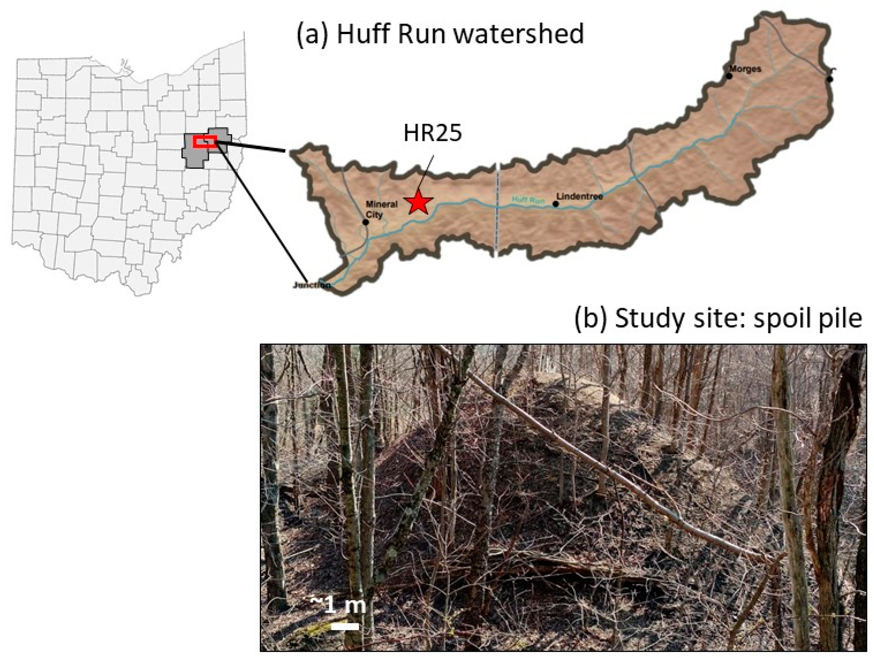
2.1. Site Description

This research was conducted in sub-watershed HR25 of the Huff Run Watershed (31.9 km2), which is located in the unglaciated portion of the Allegheny Plateau region of northeastern Ohio (Figure 1). Local lithology consists of Pennsylvanian sandstones and siltstones interbedded with claystone, limestone, and coal [32]. The Huff Run (15.9 km) flows southwest through Carroll and Tuscarawas Counties before joining the Conotton Creek near Mineral City, Ohio (OH). The lower two-thirds of the watershed were mined for coal and other resources starting in the early 1800s, with the majority of deep mining occurring between 1850–1930 [33]. Acid mine drainage (AMD) from abandoned coal operations has impaired the Huff Run and many of its tributaries and is the focus of current reclamation efforts [34].
Sub-watershed HR25 (0.44 km2) is located northeast of Mineral City and contains a 0.72-km long tributary that flows through unreclaimed coal mine spoil and receives AMD discharge from an underground coal mine that was abandoned in 1922 [34]. Numerous piles of vegetated mine spoil exist within the catchment. While some piles were capped with clay and seeded with grassy vegetation during reclamation, older piles remain unreclaimed and host forest vegetation that developed after waste emplacement. Additional small piles of mine spoil that are scattered throughout the catchment remain non-vegetated. Our research focuses on one mound of forested, unreclaimed mine spoil (~9 m tall and 26 m wide) that hosts trees but little to no grass or other understory (Figure 1).

2.2. Weather Data and Evapotranspiration Calculations

Average annual evapotranspiration (L m−2 y−1) was calculated at the scale of the Huff Run watershed as the difference between total precipitation and discharge for each year from 1998 to 2015. Precipitation records were obtained from National Trends Network site OH71 located 32 miles northwest of Mineral City, OH [35]. Reported precipitation (cm y−1) was converted to an annual volume per square land area (L m−2 y−1). Discharge (ft3 s−1) that was reported at the United States Geological Survey (USGS) site 03121850 monitoring station from 1998 until April 2015 [36] was also converted to an annual volume normalized to the drainage area (L m−2 y−1).
Evapotranspiration was also estimated by the Penman–Monteith equation using the UC Davis Daily Reference Evapotranspiration Calculation [37]. Weather data (precipitation, wind speed and direction, solar radiation) were recorded at 10-minute intervals by a micrometeorological station and EM50 datalogger (Decagon Devices, Inc.) from 1 October 2015 to 30 September 2016 (Table S1). Precipitation was measured with a tipping bucket rain gauge with 0.2-mm precision (ECRN-High Resolution Rain Gauge, Decagon Devices, Inc.). Precipitation and wind data were compared to weather data collected from a National Oceanic and Atmospheric Administration weather station at Clever Field Airport in New Philadelphia, Ohio (40.7194, –81.4236) located approximately nine miles southwest of the research site (272.8 m elevation). The anemometer in the weather station repeatedly failed to report wind speed; consequently, wind data collected at Clever Field in New Philadelphia (WBAN:04852) were used in evapotranspiration calculations. Precipitation records at Clever Field were used to replace inaccurate precipitation measurements collected at HR25 from June through September 2016. Monthly precipitation records were within 5% similarity on average between HR25 and Clever Field from October 2015 through May 2016 (Table S1).

2.3. Soil Collection and Analysis

2.3.1. Bulk Characterization

A soil core (HR25-BY1) was collected from the hilltop of the spoil pile during lysimeter installation. The core was excavated with a 2.25-inch (5.7 cm) stainless-steel bucket auger in 10-cm increments to 140-cm maximum depth. Leaf litter was removed from the land surface before the soil cores were collected, and no organic horizon was present. Collected bulk soils were air dried at room temperature in the laboratory. The dried soils were split into representative subsamples using a Riffle-type sample splitter. Each subsample was ground into a fine powder by first breaking down large rock fragments with a mortar and pestle, and then pulverizing all of the material into silt-sized particles in a Spex 8000 ball mill with tungsten carbide vials. Another unground subsample was sieved to <1 mm for particle size analysis.
Particle size analysis was completed on the <1 mm soil fraction using a Malvern Instruments Mastersizer 2000 with a Hydro 2000 MU pump accessory. Small scoops of soil were mixed with 1 L of deionized water, sonicated for 60 seconds, and pumped into the Mastersizer 2000. The relative abundance of clay-sized (<2.1 µm), silt-sized (2.1 to 67 µm), and sand-sized (67 to 1891 µm) particles were calculated as the sum of all the particles within the indicated bin size, which were set by the instrument parameters. Standard deviation was determined from the triplicate analysis of each soil.
Soil pH was measured on powdered soils mixed with either ultrapure water (pHw) or 1 mol L−1 KCl (pHKCl) in a 1:5 soil to solution mass ratio. Approximately four grams of powdered soil were mixed with 20 ml of solution in a 50-mL centrifuge tube, vortexed to mix, and then agitated for ~10 minutes. Larger soil particles were allowed to settle out of solution (~10 minutes). The pH of the supernatant solution was measured with a benchtop Orion electrode pH meter calibrated with 7.00 and 4.01 pH standards at 25 °C. Specific conductance (µS cm−1) of the supernatant solution was also measured for soils mixed with ultrapure deionized water.
Loss-on-ignition (LOI) was performed to estimate soil organic content. Approximately one gram of ground soil was combusted in a muffle furnace at 550 °C for four hours. LOI550 (% wt.) was calculated as the mass loss during combustion. Soils combusted at 550 °C were subsequently combusted at 950 °C, and loss-on-ignition at 950 °C (LOI950; % wt.) was reported as the total mass loss at 550 °C + 950 °C.
The sequential extraction protocol reported by Tessier et al. (1979) [38] was used to extract exchangeable, acid-soluble, reducible, and oxidizable Al, Ca, Fe, K, Mn, and P from soil. To obtain the exchangeable fraction, ground soil (~1 g) was mixed with 20 mL of 1 mol L−1 magnesium chloride solution (pH 7) in a 50-ml metal-free centrifuge tube. Samples were vortexed to mix and secured to an end-over-end rotator for five hours of continuous agitation. The slurries were then centrifuged at 4000 × g for 20 minutes to pelletize the soil particles. The supernatant was filtered (0.2-µm nylon filter) into a clean 50-mL centrifuge tube and acidified with one to two drops of concentrated ultrapure nitric acid (HNO3). The soil pellet was rinsed with 10 mL of ultrapure deionized water, vortexed, and centrifuged for 20 minutes. The rinse was filtered and added to the extract solution. Next, the acid-soluble fraction was extracted with 20 mL of 1 mol L−1 sodium acetate solution buffered to pH 4.75 with concentrated ultrapure glacial acetic acid. Slurries were mixed at room temperature for five hours, and then centrifuged, filtered, and rinsed. The reducible fraction was extracted with 20 mL of 0.04 mol L−1hydroxylamine hydrochloride (NH2OH·HCl) in 25% acetic acid. Slurries were heated at 96 °C for six hours and periodically agitated, then centrifuged, filtered, and rinsed. The oxidizable fraction was extracted at 85 °C for three hours with three ml of 0.02 mol L−1 HNO3 and five mL of 30% H2O2 acidified to pH 2 with ultrapure HNO3. Then, 3.4 mol L−1 of ammonia acetate was added, and the samples were continuously agitated at room temperature for an additional 30 minutes. The slurry was centrifuged, filtered, and rinsed as described previously.
All of the solutions were stored at 4 °C prior to analysis by inductively coupled plasma optical emission spectrophotometry (ICP-OES; Optima 8000). Element concentrations in extract solutions were quantified using calibration standards that were prepared in matrix solutions. All of the calibration standards were analyzed in duplicate or triplicate. Blanks were analyzed to ensure minimal contamination from the extract solution, which was defined as values either below detection or two orders of magnitude lower than in a sample extract. Element concentrations in the residual silicate fraction were determined as the difference between the bulk geochemical composition (measured by x-ray fluorescence) and the sum of the extractions. Soil concentrations were normalized to dry soil mass.

2.3.2. X-ray Absorption Spectroscopy

X-ray absorption spectroscopy (XAS) measurements were collected at beamline 12-BM at the Advanced Photon Source (Argonne National Laboratory). Powdered soils were packed into a sample holder and sealed with Kapton tape. The incident beam (~500 µm) was generated with a Si(111) monochromator to yield a reported flux of 4 × 10¹¹ s−1 @ 12 keV. XAS spectra were collected from –50 to +550 eV around the Mn K-edge (E0 = 6539 eV) in fluorescence mode using a Canberra 13-element Ge detector. Energy calibration, the merging of replicate scans, background subtraction, and normalization were completed in Athena software (Demeter v.0.9.25). All of the spectra were referenced to a zero-valent Fe foil (E0 = 7110.7 eV) [39]. Linear combination fits to normalized µ(E) spectra were performed from –20 to 30 eV around the K-edge using single-valence standards for Mn [40] to determine the average oxidation state. The sum of fitted components equaled 100% in all of the cases except for the 0–10 cm soil, where it equaled 106%; correspondingly, reported components for that soil were normalized to equal 100%.

2.4. Water Collection and Analysis

Five suction lysimeters (1900L, Soilmoisture Equipment Corp.) were installed in the spoil pile in June 2015 to depths of 10 cm, 30 cm, 50 cm, 80 cm, and 105 cm. Water collected by negative pressure lysimeters may be considered to be mobile water that infiltrates through the soil profile. Each lysimeter was constructed from polyvinyl chloride pipe and a ceramic porous cup with a maximum pore size of 1.3 µm. To install the lysimeters, the ceramic cups were set in silica slurry poured in the bottom of each excavated hole. The space around each lysimeter was backfilled with the excavated soil, and thin layers of bentonite clay pellets were placed above the silica slurry and at the soil surface to prevent preferential vertical flow. The lysimeters were capped with a rubber stopper fit with neoprene tubing and left undisturbed until pore water sampling began in March 2016.
A negative pressure gradient (–0.5 bars) was applied using a hand pump to draw soil water through the porous cup into the lysimeter. Water was extracted with an acid-washed plastic syringe and tubing that was rinsed with ~five mL of sample prior to collection. Soil water was collected from 30 March to 24 May in 2016 and from 1 April to 9 June in 2017. No soil water could be collected from June through the end of autumn due to dry conditions. Rain water (n = 2) was collected in a rain gauge that was installed in an open field on the same hilltop as the weather station.
Unfiltered soil water and rain water were analyzed on site for pH and specific conductance. Remaining water was filtered through 0.2-µm nylon filters and aliquoted into acid-rinsed plastic bottles for cation analysis (acidified with ultrapure nitric acid) and anion analysis, or into acid-rinsed and combusted amber glass vials for dissolved organic carbon analysis (acidified with ultrapure hydrochloric acid). Water was stored at 4 °C prior to analysis. Dissolved cations (Al, Ca, Fe, K, Mg, Mn, and P) were analyzed by ICP-OES. Anions (Br⁻, Cl⁻, F⁻, NO₃⁻, SO₄2⁻, and PO₄3⁻) were measured on a ThermoScientific Dionex ICS-2100 using 30 mmol L⁻1 potassium hydroxide eluent. Dissolved organic carbon (DOC) was measured by the combustion method on a Shimadzu TOC-L analyzer.

2.5. Vegetation Collection and Analysis

All of the trees growing on the spoil pile were tagged and identified (Table S2). Diameter at breast height (DBH, cm) was measured at 1.3 m with a DBH measuring tape (Forestry Suppliers, Inc.). Leaf biomass was calculated as a function of DBH using a reported allometric equation [41]. Green leaves were sampled throughout the growing season from trees growing on the spoil pile. The green leaves were collected by using a pole cutter to snip the highest reachable tree branches in the mid-to-upper canopy. Understory was sparse on the hill and was not included in biomass calculations. Leaf litter samples were collected weekly to biweekly from 3 October to 20 November 2016 from five leaf litter traps installed one meter above the ground surface at the same sites where green leaves were sampled (Table S3). Leaf litter traps were constructed from plastic rectangular containers (0.262 m2) with drainage holes drilled in the bottom and plastic mesh lining (1.27 cm × 1.90 cm) secured to the inside of the container with zip-ties.
Green leaves and leaf litter were air-dried in the laboratory. A subsample of the homogenized material was powdered in the ball mill. The high temperature dry oxidation method was used to prepare the plant leaf tissue for the quantitative determination of the concentrations of metals in the green leaves [42]. Precisely 0.5 g of ground material was combusted at 550 °C for four hours, and the ash was dissolved in 10.0 mL of 1.0 mol L−1 HNO3 solution in a 15-mL falcon tube. Then, three mL of concentrated (~34%) ultrapure hydrogen peroxide (H2O2) was added, and the mixture was heated at 85 °C to dissolve the remaining organic matter. Samples were filtered (<0.45 µm) prior to analysis by ICP-OES for Mn, Fe, Al, K, Mg, Ca, and P. A reference standard (NIST SRM 1570a spinach leaves) was also ashed and dissolved in nitric acid following the same procedure.

2.6. Mass Balance Model

A mass balance model was used to calculate annual fluxes to and from the system (atmospheric deposition and leaching) and internal cycling between soil and vegetation. Here, the system was defined as the soil core extending from the land surface (0 cm) to the maximum core depth (140 cm), which we take to represent one square meter of surface area for a total volume of 1.40 m3. Since we are considering fluxes that occur over short subdecadal timescales, we do not include inputs from bedrock weathering or losses to soil erosion. The mass of each element in the soil core, Mi, was calculated as the product of total element concentration (mmol kg−1), core depth (m), and soil bulk density (~1500 kg m−3).
Atmospheric deposition inputs (A, mmol m−2 y−1) were calculated as the product of the concentration of each species (subscript i) measured in precipitation (Ci,p, mmol L−1) and the volume of precipitation that fell on one square meter of land surface each year (Vp, L m−2 y−1):
A i = C i , p × V p
Mass loss from the soil in chemical weathering (Wi, mmol m−2 y−1) was calculated as the product of the concentration of each species i measured in soil water at 105-cm depth (Ci,w, mmol L−1) and the volume of water that drained through the soil profile each year (Vd, L m−2 y−1):
W i = C i , w × V d
Here, Vd (430 ± 160 L m−2 y−1) was determined from discharge recorded in the Huff Run at Mineral City (USGS site 03121850), which comprised 44.9% ± 11.9% of annual precipitation for the period of record between 1998–2015. Annual precipitation averaged 95.1 ± 13.5 cm y−1, as measured at the National Atmospheric Deposition Program (NADP) site OH71. An independent value for Vd was also calculated as the difference between Vp and the volume of water lost to the atmosphere through evapotranspiration (VET, L m−2 y−1), which was calculated using the Penman–Monteith model. The models that were used to calculate ET produced Vd values less than watershed-scale Vd, and two out of three models produced values exceeding annual precipitation; therefore, we use the Vd value determined as the watershed-scale as an upper bound on the volume of water infiltrating the soil profile. The lower bound on Wi for each element would then be zero in a scenario where all of the precipitation was lost to evapotranspiration, and none could infiltrate; however, this is unlikely, since water collected in the lysimeters below the rooting zone during periods of the year. Low infiltration values that were obtained using the Penman–Monteith calculation indicated that ET reduced infiltration through the spoil.
Element cycling out of and into the system occurred each year through uptake by vegetation and subsequent litterfall. Uptake by vegetation (Ui, mmol m−2 y−1) was calculated as the product of the concentration of each species i measured in green foliage (Ci,f, mmol kg−1) and the area-normalized mass of foliage on the hill (mf, kg m−2):
U i = C i , f × m f
Foliar mass was determined using an allometric equation that derives leaf mass for each tree from the diameter at breast height [41].
Element return to the soil in litterfall (Li, mmol m−2 y−1) was calculated as the product of the concentration of each species i measured in leaf litter (Ci,l, mmol kg−1) and the total area-normalized mass of leaf litter that collected in littertraps over the autumn (ml, kg m−2):
L i = C i , l × m l
Uptake and litterfall calculations assume that elements are delivered from pore water to the leaves each year and subsequently deposited back to the soil in leaf litter with relatively low retention in the standing biomass. Although Mn and Ca are preferentially translocated into foliage and are not reabsorbed during senescence [43,44], non-negligible quantities may be stored in woody tissue each year and contribute to longer retention times in standing biomass.

3. Results

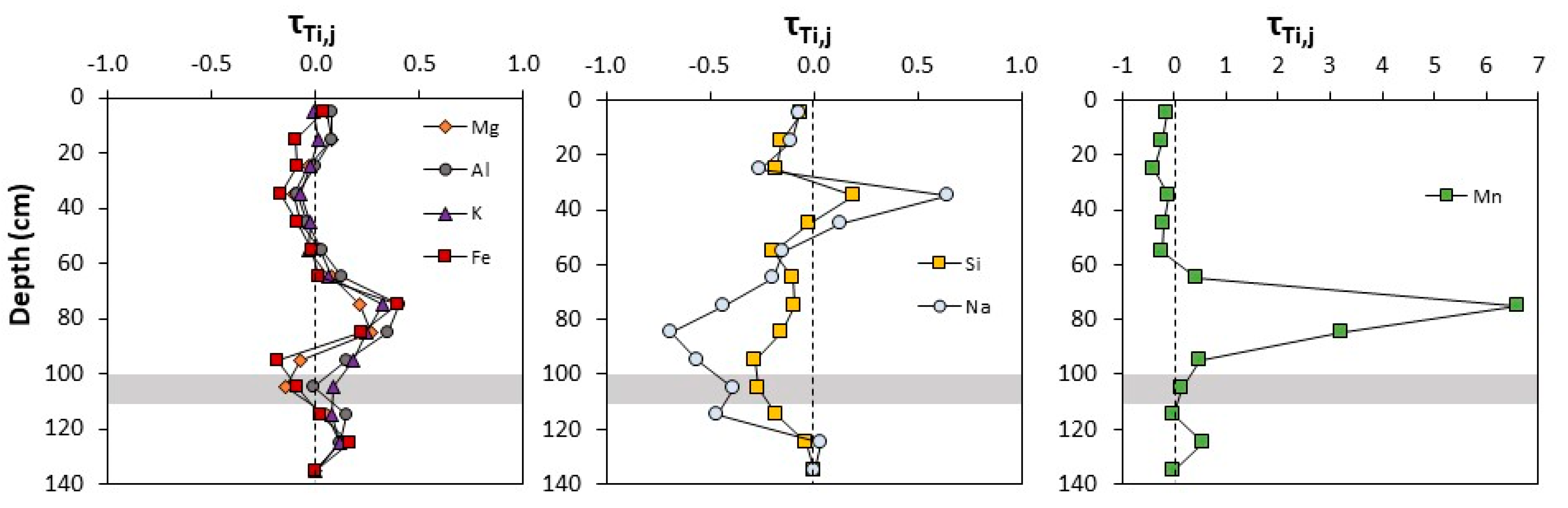
3.1. Soil Geochemistry

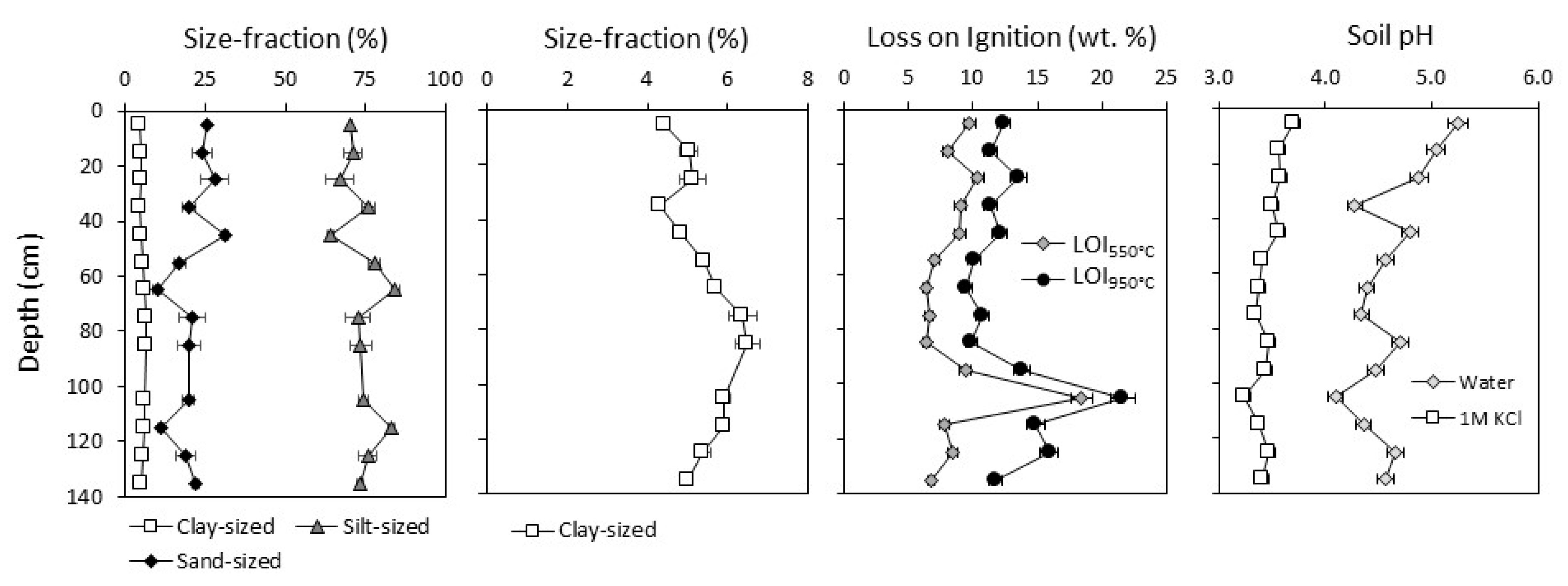
3.1.1. Soil Properties

Soil geochemistry and physical properties varied with depth in the soil profile, indicating the presence of heterogeneous soil layers (Figure 2). Soil had a silt loam texture at all of the depths that varied by <20% in the proportions of silt-sized and sand-sized fractions. The clay-sized fraction increased with depth and was highest (6.5% ± 0.3%) between 80–90 cm before declining to 5.0% in the deepest soil. Loss-on-ignition at 550 °C ranged from 6.4 to 10.4 wt.% across all of the depths with a pronounced peak of 18.4 wt.% between 100–110 cm. Loss-on-ignition at 950 °C was ~2–4 wt.% higher than LOI550 at all of the depths except between110–130 cm, where it was ~7 wt.% higher. Soil was acidic (pHH2O = 5.3 ± 0.1) at the surface, and pHH2O decreased with depth to a minimum pH of 4.1 ± 0.1 between 100–110 cm. Exchangeable acidity was higher but less variable across all of the depths, yielding pHKCl values that decreased from 3.7 near the surface to 3.2 between 100–110 cm.
Major soil elements exhibited distinct depth profiles that varied both in total concentration (Table 1) and in the proportions of different extracted phases (Figure 3; Table S4). Averaged across all depths, Si (9750 ± 640 mmol kg−1), Al (3340 ± 490 mmol kg−1), and K (774 ± 105 mmol kg−1) were the most abundant elements, which is consistent with a soil composed of (alumino)silicate minerals. Soil Fe (908 ± 128 mmol kg−1) was also high, while base cations Mg (275 ± 35 mmol kg−1), Na (145 ± 50 mmol kg−1), and Ca (< DL) were relatively low. Titanium concentrations were low (68 ± 6 mmol kg−1) and varied little with depth. Soil Mn was distinct from the other major elements in that it was low through the soil profile (<10 mmol kg−1) with the exception of a Mn-rich layer between 70–80 cm where concentrations increased to 46 mmol kg−1.
The mass transfer coefficient, τi,j, was used to evaluate depth profiles for mobile elements (subscript j) in the weathered soil (subscript w) normalized to an immobile element (i = Ti) and to the parent material (subscript p) [45,46,47]:
τ i , j = ( C j , w × C i , p ) / ( C j , p × C i , w ) 1
Here, we assumed that the soil profile weathered from a homogeneous parent material with a composition represented by the deepest sample (130–140 cm), and that variation in τi,j values derived from weathering processes that occurred after the spoil was deposited. It is also possible that heterogeneous layers of material were sequentially deposited during mining excavation, in which case τi,j variation would derive at least partially from differences in source material relative to the deepest sample.
The major elements Al, K, Fe, and Mg had similar depth profiles, with small depletions (τTi,j <0) occurring in shallow soils, but enrichment (τTi,j >0) occurring between 60–90 cm (Figure 4; Table 2). This trend was similar to the depth distribution of clay-sized particles (Figure 2). In contrast, Si and Na showed enrichment between 30–40 cm, but depletion from 50 to 130 cm. Maximum Na depletion (~70% depleted) was higher than for Si (~30% depleted). Soil Mn was unique, with slight depletion occurring near the surface but strong enrichment below 60 cm, reaching as high as τTi,Mn = 6.6 from 70–80 cm. This enrichment occurred in the clay-rich layer that was also slightly enriched in Mg, K, Al, and Fe, but depleted in Na and Si.

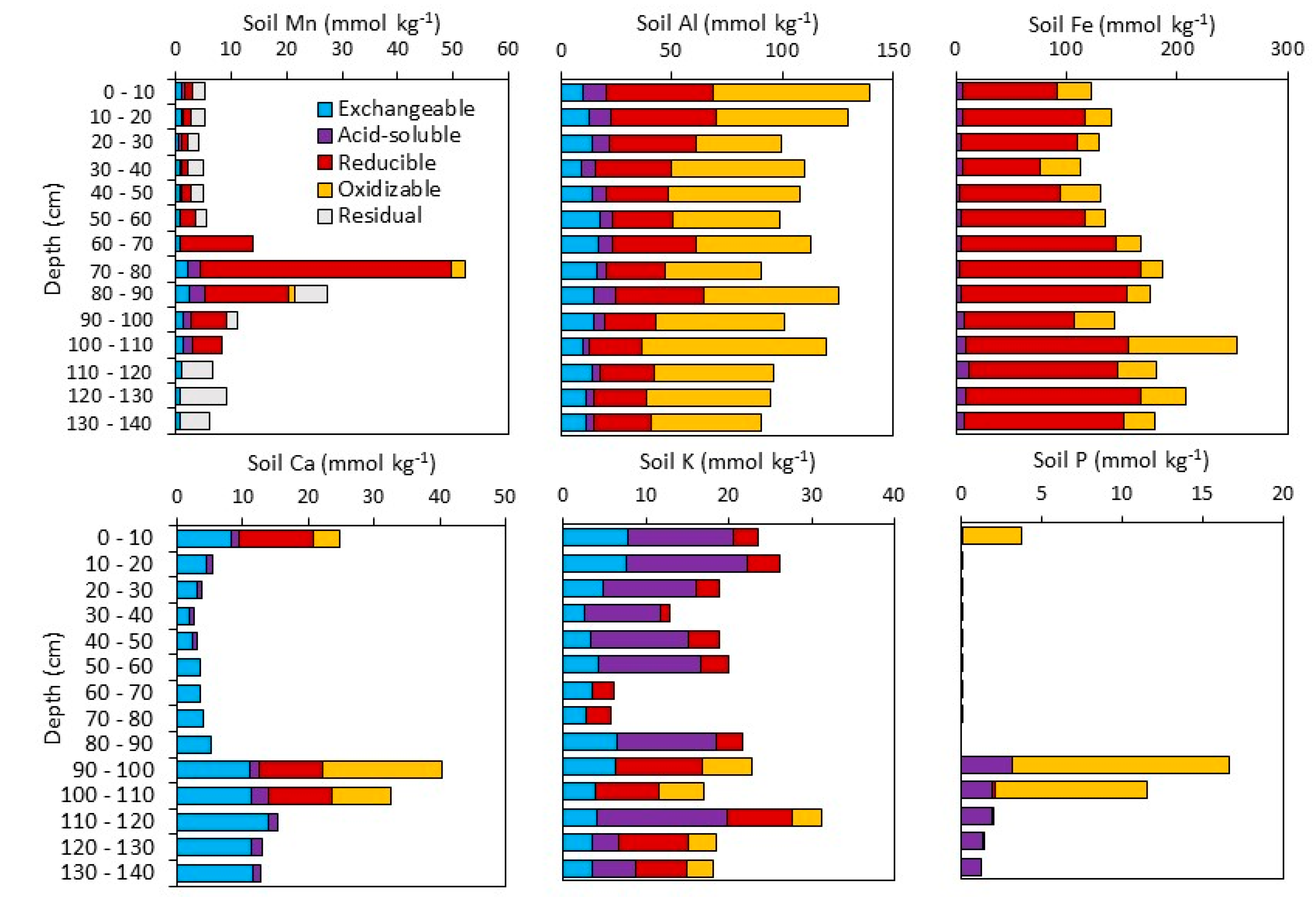
3.1.2. Sequential Extractions
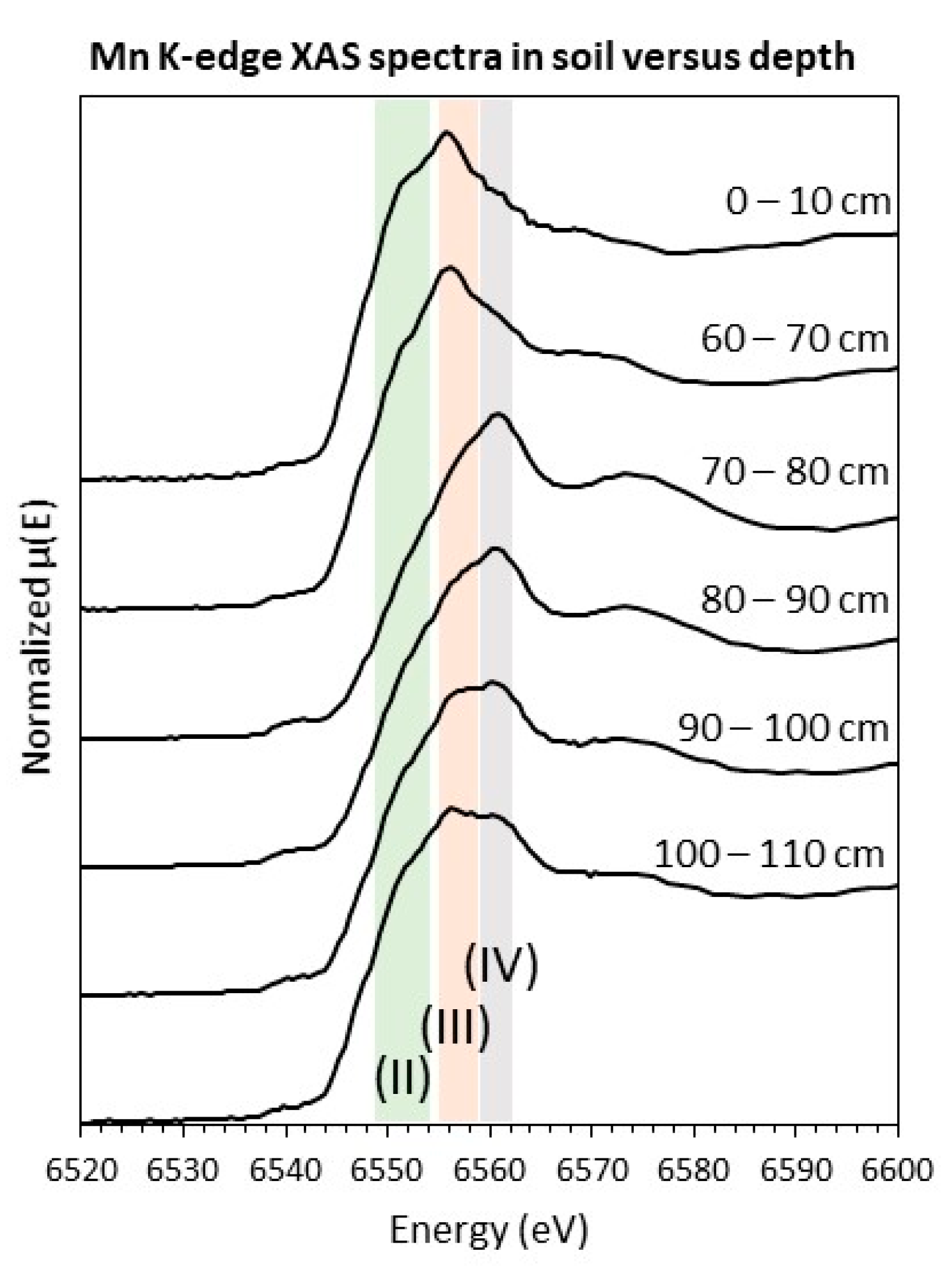
Reducible Mn comprised the majority of Mn in the Mn-enriched zone (Figure 3). Shallower, Mn-poor soils contained <50% reducible Mn, while no reducible Mn was detected below 110 cm. Exchangeable Mn concentrations were also highest in the enriched zone but comprised a smaller proportion of total Mn (<10%) than in shallower soils (up to 23%). Oxidizable Mn was only detected in the Mn-rich zone between 70–90 cm, and residual Mn was the primary phase in the deepest soils.
Iron, Al, and K were primarily present in the residual fraction (Table S4), which is consistent with their occurrence in silicate minerals. Reducible Fe comprised 13.4% ± 2.4% of total Fe and increased slightly with depth, whereas oxidizable Fe was relatively low (3.9% ± 2.5% of total Fe) at all of the depths except the 100–110 cm soil layer (11.2% of total Fe) (Figure 3). Exchangeable and acid-soluble Fe comprised <1% of total Fe. Extractable Al decreased slightly with depth and was present mainly in the reducible and oxidizable fractions with smaller quantities of exchangeable and acid-soluble Al. Only small quantities of soil K (<2%) could be extracted, and these were distributed amongst the different fractions with oxidizable K present only below 90 cm.
Soil Ca was low (average sum of extracted phases = 12 ± 12 mmol kg−1) and present mainly in the exchangeable fraction with contributions of reducible and oxidizable Ca present at the surface and from 90–110 cm depth. Low concentrations (<3 mmol kg−1) of acid-soluble Ca were present at <50 cm and >90-cm depth. Soil P was below detection in most of the soil profile with the exception of oxidizable P in the surface and from 90–110 cm, and <4 mmol kg−1 acid-soluble P below 90 cm. Some major elements were not measured in the extracted fractions due to either their presence in extract solution (Na, Mg) or their low solubility (Si, Ti).

3.1.3. Spectroscopy

X-ray absorption spectroscopy was used to investigate Mn speciation in surface soil (0–10 cm) and in soils spanning the Mn-rich layer (60–70 cm, 70–80 cm, 80–90 cm, 90–100 cm, and 100–110 cm) (Table S5). A Mn K-edge spectrum from the Mn-rich layer (70–80 cm) was consistent with Mn (IV) oxides such as birnessite (Figure 5a) and yielded an average Mn oxidation state of +3.66 (Table 3). Soils above and below the Mn-rich layer contained higher proportions of Mn(II) and Mn(III) species, which was evident by a shift of the µ(E) peak to lower energy and by increasing absorbance in the Mn(II) region (Figure 5a). Correspondingly, the average Mn oxidation state in these layers ranged from 2.5 to 3.4 (Table 3). These results are consistent with an abundance of reducible Mn(IV)-oxides in Mn-rich layers, but exchangeable Mn2+ and Mn(II)-bearing silicates in Mn-poor layers (Figure 3) [48,49].

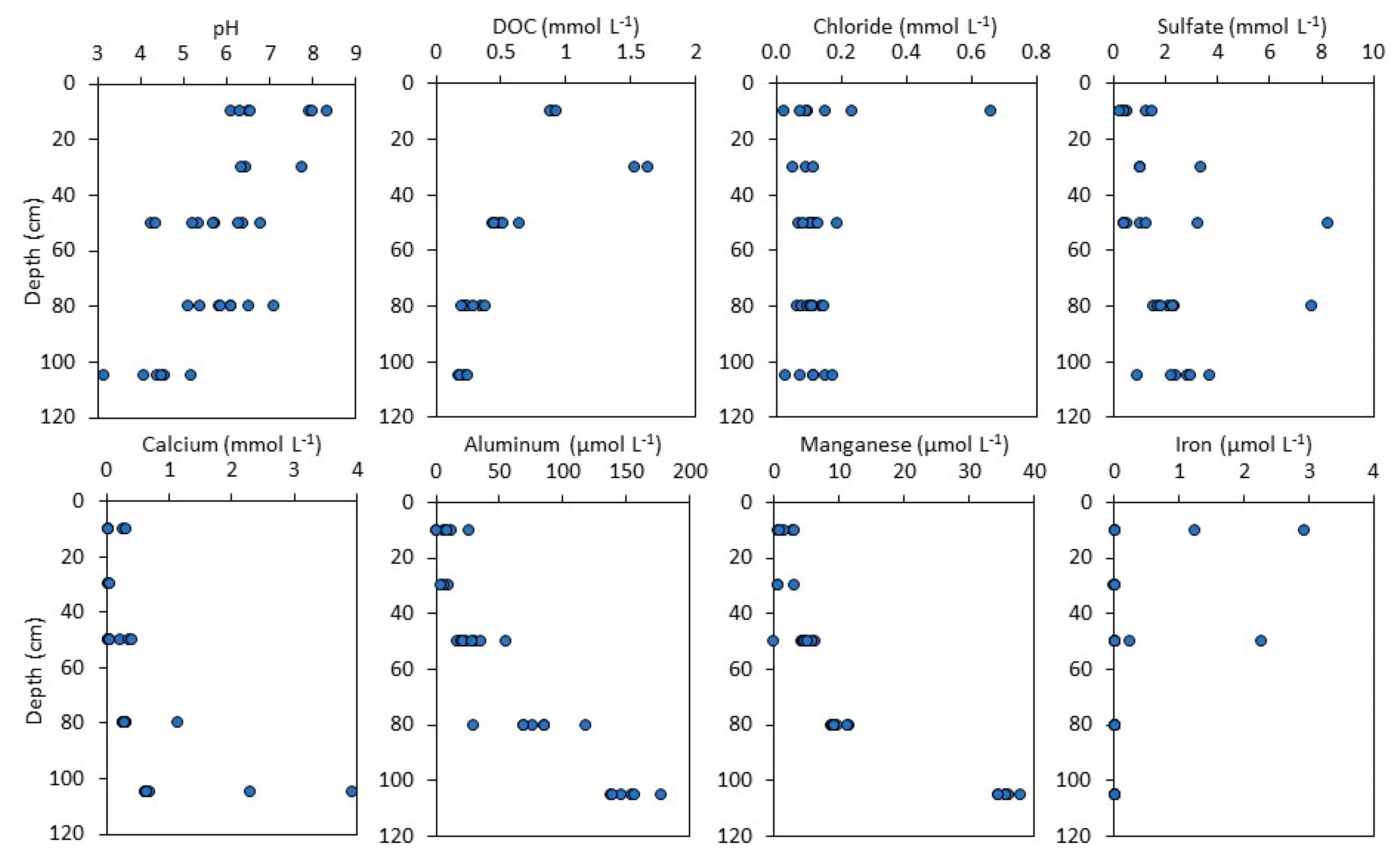
3.2. Soil Water Chemistry

Soil water was circumneutral near the surface but increasingly acidic with depth, reaching pH values as low as 3.2 at 105 cm (Figure 6; Table S6). At each depth, pH varied by approximately two units. Iron and DOC were higher in shallow soils than at depth, and dissolved Fe was typically below detection in deeper soils. Dissolved Mn, Al, and Ca concentrations were low above 60 cm, but increased by a factor of three at 105 cm, reaching concentrations as as high as 38 µM, 177 µM, and 3.9 mM, respectively. Sulfate increased slightly with depth and was highly variable, typically < 3.0 mmol L−1 but reaching concentrations as high as 8.3 mmol L−1. Chloride concentrations (0.13 ± 0.11 mmol L−1) were similar across all of the depths, which is consistent with a conservative (non-reactive) behavior. Rain water was below detection for all of the metals (<0.01 µM).

3.3. Vegetation Chemistry

Forty-nine trees with DBHs ranging from 1.6 to 61.2 cm (median = 5.0 cm) were identified growing on the spoil pile (Table S2). Seventy-five percent of the trees were identified as red maples (Acer rubrum; n = 37). The remaining trees were identified as American elm (Ulmus americana), autumn olive (Elaeagnus umbellata), bitternut hickory (Carya cordiformis), black cherry (Prunus serotina), black oak (Quercus velutina), choke cherry (Prunus virginiana), common dogwood (Cornus sanguinea), and sassafrass (n ≤ three each). Foliar biomass that accumulated over the growing season was calculated as 480 g m−2 y−1 averaged over the canopy area ([41]; Table S2).
Foliar Ca (170 ± 14 mmol kg−1) and Fe (0.94 ± 0.09 mmol kg−1) were within the normal ranges reported for each element in mature leaf tissue [50]. In contrast, foliar Mn (25 ± 2 mmol kg−1) and Al (3.4 ± 1.3 mmol kg−1) exceeded standard and/or healthy ranges (0.4 to 5.4 mmol kg−1 for Mn [50]; 2.4 mmol kg−1 for Al [51]). Foliar Al may even have been underestimated by as much as ~50%, given that Al recovery on ashed and acid-digested NIST-1570a reference material was only 53%. Better recoveries were obtained for Mn and Ca (80–85%).
Leaf litter deposition averaged 8.6 ± 5.3 g m−2 d−1 from 6 October through 10 November, yielding an estimated total deposition of 302 ± 185 g m−2 litter mass during that time (Table S3). This value was similar to the estimated foliar biomass at our site and to the annual litter deposition reported for a comparable but undisturbed, shale-underlain temperate forest in Pennsylvania (384 g m−2 y−1) [29]. It is possible that litter deposition was slightly underpredicted, because no litter was collected in September or late November; however, these early and late dates likely only represent a small portion of collected leaves. Litter may also have moved laterally off the steep hill, resulting in mass transfer from the hilltop downslope. Litter chemistry was similar to green leaf chemistry for Ca (234 ± 129 mmol kg−1), Mn (21.9 ± 8.0 mmol kg−1), Fe (1.2 ± 0.3 mmol kg−1), and Al (1.8 ± 0.8 mmol kg−1), indicating negligible change during senescence.

4. Discussion

4.1. Soil and Pore Water Geochemistry

The weathered mine spoil was characterized by physically and geochemically distinct layers that reflect the pedogenic weathering processes following spoil deposition. Notably, a reaction front was observed at approximately 90-cm depth, where soil enriched in weathering products (clays and metal oxides) transitioned to deeper soil enriched in reduced materials (organic matter, metals in oxidizable soil fractions). Between 70–90 cm, clay enrichment was indicated by an increase in clay-sized particles (Figure 2), residual Fe and Al, and total Fe, Al, K, and Mg (Figure 3). Metal oxide enrichment was indicated by high concentrations of reducible Mn and Fe (Figure 3), and Mn K-edge XAS spectra consistent with birnessite (Figure 5). These results indicate the presence of a soil layer where metal oxides and clay particles have accumulated following precipitation and translocation, respectively. Similar subsurface distributions of organic matter, Fe and Mn, were observed in a spoil pile located approximately 20 m from this study site (Figure S1).
An exceptionally organic-rich layer was present at 105 ± 10 cm depth, which is coincident with increased soil acidity, decreased total cation concentrations, and increased concentrations of oxidizable elements (Fe, Ca, K, and P) (Figure 2 and Figure 3). We infer that this layer is composed of high amounts of organic-rich coal and black shale that contain reduced minerals such as sulfides. The persistence of reduced minerals indicates that pyrite oxidation within these soils continues to produce a non-point source of pollution after nearly a century of weathering. Indeed, sulfide oxidation can also explain the high concentrations of dissolved metals (Mn, Al) and acid within this layer (Figure 6). These metals could be released from the reduced materials (sulfides and organics) during oxidative weathering or dissolved from other minerals such as oxides and aluminosilicates due to the increased acidity. For example, Mn can substitute into pyrite and be mobilized when pyrite dissolves [52,53]. The organic-rich layer contained increasing proportions of Mn(II) that may in part derive from Mn(II)-bearing pyrite (Figure 5), although the specific phase could not be identified here. Although concentrations of dissolved Mn increased just below the Mn-rich layer, indicating some dissolution and leaching from Mn oxides, they again tripled in the organic-rich layer, suggesting mobilization from a reduced phase contained within this soil (Figure 6). Consequently, the Mn that leached from the soil was derived primarily from the organic-rich layer rather than the Mn-oxide layer. Although Mn-oxides were present in greater abundance than trace sulfide phases, sulfides weather rapidly in the presence of water and oxygen and could disproportionately contribute to high dissolved Mn. Dissolved Al increased linearly with depth from 30 to 105 cm, implicating an aluminosilicate source rather than any minerals that were present strictly within the coal-rich layer (Figure 6). Although sulfate concentrations increased only slightly with depth, it is likely that sulfate concentrations produced by sulfide oxidation were much lower than the sulfate derived from atmospheric deposition and cannot provide a tracer for sulfide oxidation.
The deep, organic-rich layer also had low concentrations of DOC, indicating that the organic material was insoluble and not readily leached into solution, which is consistent with geologic C contained in refractory coal [54]. Dissolved organic C was instead highest in shallow soils where the decomposition of young leaf litter released labile organic molecules into solution (Figure 6). Recent plant-derived organic molecules can be degraded by microorganisms during soil water infiltration or may adsorb to coal particles in the subsurface [55].
In contrast to Mn, dissolved and exchangeable Fe were generally below detection. Spikes in dissolved Fe occurred only sporadically in shallow soils that were depleted in Fe relative to deep soils (Figure 6). Iron mobility in shallow soils was likely controlled by the formation of organic complexes, e.g., through ligand-promoted and/or the reductive dissolution of iron oxides. High concentrations of DOC in shallow soils may mobilize Fe through these means. Fe complexes may have been translocated downward in the soil where the Fe was released and precipitated as Fe oxides, contributing to subsurface Fe accumulation (Figure 3). Although the organic-rich layer contained a large fraction of oxidizable Fe, presumably as Fe sulfides, low concentrations of dissolved Fe at depth indicate that any Fe produced by sulfide oxidation also readily precipitated as iron oxides.
The depth trends that were observed for other elements support these interpretations. Non-silicate Al was primarily associated with soil organic matter (oxidizable Al), while lesser amounts were substituted into reducible Fe and Mn oxides. High concentrations of dissolved Al in deep soils were favored by the high soil acidity, and may have derived from either the acid dissolution of silicates or the oxidation of organic-bound Al. Phosphorus was low throughout the profile with the exception of high concentrations of oxidizable P in the surface soil and in the coal-rich layer at depth, representing P contained in soil organic matter and old, refractory organic material, respectively. Low concentrations of acid-soluble P in the deepest soils could represent apatite that has weathered completely out of shallow soils.

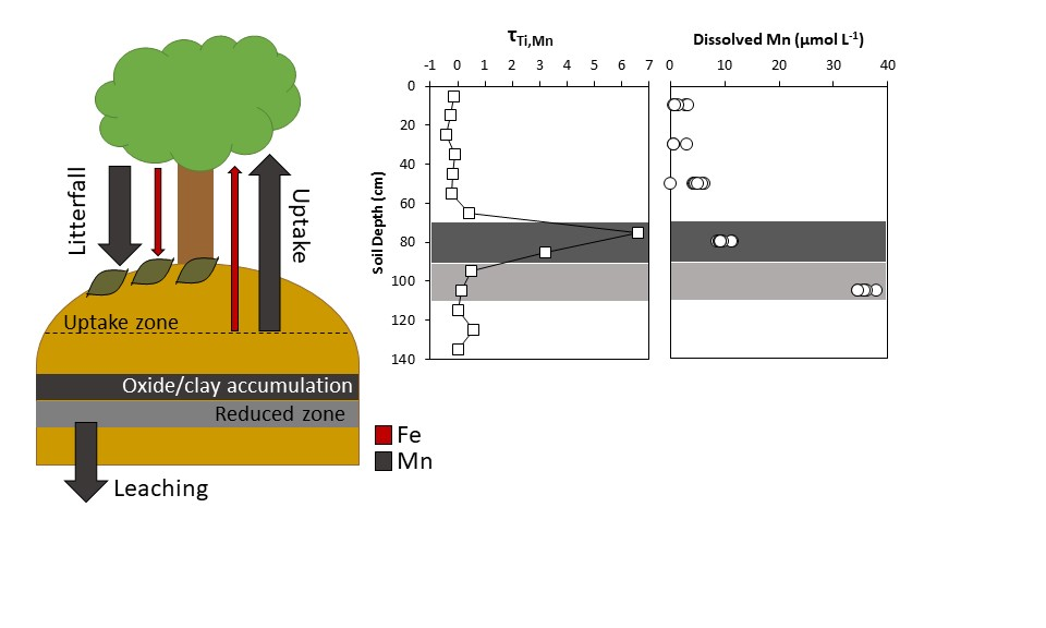
4.2. Biogeochemical Cycling between Plants and Mine Spoil

Iron and Mn exhibited distinct biogeochemical signatures that reflect the contrasting effects of forest vegetation. Specifically, biocycling by trees influenced Mn cycling to a far greater extent than that observed for Fe. Foliar Mn concentrations were 27× higher than foliar Fe concentrations even though soil Mn concentrations were equal to only ~1% of soil Fe (Table 1 and Table S2). Thus, trees accumulated large quantities of Mn, but only small amounts of Fe. Shallow soils contained high proportions of exchangeable Mn2+ that provide a readily bioavailable source (Figure 3 and Figure 5) and low concentrations of pore water Mn due to plant uptake (Figure 6). Although biocycling can lead to Mn enrichment in shallow soils [29,50,56], the soil examined here lacked the surface accumulation of organic matter that is needed to reintroduce Mn into the shallow soil. In contrast, forest vegetation accumulated little Fe, but the leaching of leaf litter provided high concentrations of dissolved organic molecules in shallow soils that increased Fe mobility (Figure 6).
A mass balance model was used to evaluate the biogeochemical cycling of Mn and Fe through forest vegetation relative to inputs to and outputs from the plant–soil system (Table 4). The plant uptake of Mn (UMn = 12 ± 1 mmol m−2 y−1) and return to the soil in litterfall (LMn = 6.6 ± 2.4 mmol m−2 y−1) were within the estimated range for Mn leaching from the soil profile via chemical weathering (WMn <15 ± 7 mmol m−2 y−1). Although Fe was ~100x more abundant than Mn in the soil, plant uptake (0.45 ± 0.04 mmol m−2 y−1) and litterfall (0.36 mmol m−2 y−1) fluxes for Fe were two to 20 times lower than for Mn, indicating minimal plant recycling. Iron leaching was negligible (<0.01 mmol m−2 y−1), because Fe concentrations in pore water were below detection. Wet atmospheric deposition for both elements was assumed to be zero, because metal concentrations in rain water were below detection.
Aluminum and Ca fluxes were evaluated for comparison. Aluminum had low cycling through vegetation (UAl = 1.6 ± 0.6 mmol m−2 y−1 and LAl = 0.55 ± 0.23 mmol m−2 y−1), although these values may be underestimated due to the low recovery of Al in leaf digests. Weathering losses of Al were relatively high (WAl = 65 ± 24 mmol m−2 y−1) and reflect high Al concentrations in deep, acidic pore waters. Relative to these metals, the major nutrient Ca had high uptake (UCa = 82 ± 7 mmol m−2 y−1) and litterfall fluxes (71 ± 39 mmol m−2 y−1). Leaching losses were also high (WCa = 630 ± 230 mmol m−2 y−1) and far exceeded rainfall inputs (ACa = 4.3 ± 0.7 mmol m−2 y−1).
Uptake and weathering fluxes (mmol m−2 y−1) were normalized to Mi (mol m−2), the mass of the element in the soil core, to calculate the fraction of each element present in the soil that was taken up by plants or leached by chemical weathering each year (y−1) (Table 4). The annual fractions of soil Mn that were either cycled through vegetation (52 ± 4 × 10⁻⁵ y−1) or chemically weathered and leached (67 ± 25 × 10−5 y−1) were orders of magnitude higher than those for Fe (0.02 ± 0.001 × 10⁻⁵ y−1 and <0.02 × 10⁻⁵, respectively). The fractions of biocycled and weathered Al were also quite small (< 1 × 10⁻⁵ y−1), reflecting the high proportion of immobile Al contained in silicate minerals. Greater fractions of Ca were biocycled (340 ± 29 × 10−5 y−1) and leached (2570 ± 954 × 10−5 y−1), reflecting high concentrations of exchangeable Ca.
Forest vegetation growing on spoil effectively accumulated and recycled mobile Mn. Foliar Mn concentrations were approximately five times higher than a reported healthy range [50] and similar to concentrations in deciduous forests growing on comparably acidic soils [57,58,59,60]. Previous studies have demonstrated that vegetation strongly regulates Mn export from watersheds in systems where Mn is readily bioavailable [29,60,61,62], and vegetation may play a similar role in modulating Mn losses from soils in mining-impacted watersheds. Indeed, Mn uptake rates (12 ± 1 mmol m−2 y−1) and the fraction of soil Mn taken up by plants each year (52 ± 4 × 10⁻⁵ y−1) were consistent with the values that had been reported for a temperate deciduous forest developed on undisturbed shale (18 ± 4 mmol m−2 y−1 and 75 ± 21 × 10−5 y−1, respectively) [29]. However, the fraction of Mn leached from the HR25 soil (67 ± 25 × 10−5 y−1 upper estimate, or ~15 × 10−5 y−1 lower estimate) far exceeded that in the undisturbed watershed (2.8 ± 0.7 × 10⁻⁵ y−1). The higher Mn leaching fluxes at HR25 derived from pockets of readily weatherable Mn-bearing minerals present at one meter depth in the soil), which is likely deeper than the soil layer where the trees would access water and nutrients. Humid temperate forests, and Acer species in particular, rely primarily on shallow soil water (<60 cm depth) rather than deeper soil or groundwater sources [63]. Consequently, although biocycling by forest vegetation can mitigate Mn leaching, its influence is limited to the effective rooting depth.

5. Conclusions

Vegetated coal mine spoil abandoned nearly a century ago in the Appalachian region contained reduced materials that continued to weather and release metals into solution, potentially contributing to the non-point source contamination of nearby water bodies. Our results indicated that forest vegetation growing on coal spoil influenced metal leaching through multiple processes. First, dissolved organic molecules derived from plant material increased Fe solubility in shallow soils; however, Fe was effectively retained in these well-drained soils via precipitation as iron oxyhydroxides. Second, vegetation partially mitigated Mn leaching by accumulating large quantities of mobile Mn from shallow soils and storing it in foliage. Evapotranspiration may also reduce metal leaching by limiting rain water infiltration through the forested spoil. Circumventing retention by vegetation, high concentrations of dissolved Mn were mobilized in deeper soils, presumably resulting from the oxidative dissolution of reduced materials, and leached from the soil. Although vegetation can partially offset leaching, spoil piles may serve as long-term sources of Mn in mining-impacted systems.

Supplementary Materials

The following are available online at https://www.mdpi.com/2571-8789/3/1/13/s1, Figure S1, Tables S1–S6.

Author Contributions

Conceptualization, E.H. and D.S.; Methodology, E.H., B.Y., H.F.; Formal Analysis, E.H., B.Y., H.F.; Resources, E.H., D.S.; Writing-Original Draft Preparation, E.H., B.Y., H.F.; Writing–Review and Editing, E.H., D.S.; Project Administration, E.H.; Funding Acquisition, E.H.

Funding

This research was funded by the Farris Family Innovation Award to E.M.H. from Kent State University.

Acknowledgments

The authors would like to acknowledge Daniel Wood, Bryan Agee, Laura Zemanek, and Mallory Klein for assistance with sample collection and processing, and Nicholas Johnson for technical assistance. We thank Marissa Lautzenheiser and the Huff Run Watershed Restoration Partnership for site access and logistical support, and Chad Kinney for assistance with plant identification. Beamline support at 12-BM was provided by Benjamin Reinhart. This research used resources of the Advanced Photon Source, a U.S. Department of Energy (DOE) Office of Science User Facility operated for the DOE Office of Science by Argonne National Laboratory under Contract No. DE-AC02-06CH11357.

Conflicts of Interest

The authors declare no conflict of interest. The funders had no role in the design of the study; in the collection, analyses, or interpretation of data; in the writing of the manuscript, and in the decision to publish the results.

References

  1. U.S. Department of the Interior. Office of Surface Mining Reclamation and Enforcement. Available online: https://www.osmre.gov/ (accessed on 10 November 2018).
  2. U.S. Congress. Surface mining control and reclamation act of 1977. Public Law 1977, 95, 30. [Google Scholar]
  3. Dixon, E.L.; Bilbrey, K. Abandoned Mine Land Program: A Policy Analysis for Central Appalachia and the Nation; AML Policy Priorities Group; Appalachian Citizen’s Law Center, The Alliance for Appalachia: Whitesburg, KY, USA, 2015. [Google Scholar]
  4. U.S. Environmental Protection Agency. The Effects of Mountaintop Mines and Valley Fills on Aquatic Ecosystems of the Central Appalachian Coalfields; EPA/600/R-09/138F; U.S. Environmental Protection Agency: Washington, DC, USA, 2011.
  5. Cravotta, C.A. Dissolved metals and associated constituents in abandoned coal-mine discharges, Pennsylvania, USA. Part 1: Constituent quantities and correlations. Appl. Geochem. 2008, 23, 166–202. [Google Scholar] [CrossRef]
  6. Blowes, D.W.; Jambor, J.L. The Pore-Water Geochemistry and The Mineralogy of The Vadose Zone of Sulfide Tailings, Waite-Amulet, Quebec, Canada. Appl. Geochem. 1990, 5, 327–346. [Google Scholar] [CrossRef]
  7. Nordstrom, D.K. Hydrogeochemical processes governing the origin, transport and fate of major and trace elements from mine wastes and mineralized rock to surface waters. Appl. Geochem. 2011, 26, 1777–1791. [Google Scholar] [CrossRef]
  8. Akcil, A.; Koldas, S. Acid Mine Drainage (AMD): Causes, treatment and case studies. J. Clean. Prod. 2006, 14, 1139–1145. [Google Scholar] [CrossRef]
  9. Gray, N.F. Environmental impact and remediation of acid mine drainage: A management problem. Environ. Geol. 1997, 30, 62–71. [Google Scholar] [CrossRef]
  10. Johnson, D.B.; Hallberg, K.B. Acid mine drainage remediation options: A review. Sci. Total Environ. 2005, 338, 3–14. [Google Scholar] [CrossRef] [PubMed]
  11. Singer, P.C.; Stumm, W. Acidic mine drainage: The rate-determining step. Science 1970, 167, 1121–1123. [Google Scholar] [CrossRef] [PubMed]
  12. Moses, C.O.; Nordstrom, D.K.; Herman, J.S.; Mills, A.L. Aqueous pyrite oxidation by dissolved oxygen and by ferric iron. Geochim. Cosmochim. Acta 1987, 51, 1561–1571. [Google Scholar] [CrossRef]
  13. Evangelou, V.P. Pyrite Oxidation and Its Control; CRC Press, Taylor Francis Group: Boca Raton, FL, USA, 1995. [Google Scholar]
  14. Dang, Z.; Liu, C.; Haigh, M.J. Mobility of heavy metals associated with the natural weathering of coal mine spoils. Environ. Pollut. 2002, 118, 419–426. [Google Scholar] [CrossRef]
  15. Cravotta, C.A. Dissolved metals and associated constituents in abandoned coal-mine discharges, Pennsylvania, USA. Part 2: Geochemical controls on constituent concentrations. Appl. Geochem. 2008, 23, 203–226. [Google Scholar] [CrossRef]
  16. Hallberg, K.B.; Johnson, D.B. Biological manganese removal from acid mine drainage in constructed wetlands and prototype bioreactors. Sci. Total Environ. 2005, 338, 115–124. [Google Scholar] [CrossRef] [PubMed]
  17. Jamieson, H.E.; Walker, S.R.; Parsons, M.B. Mineralogical characterization of mine waste. Appl. Geochem. 2015, 57, 85–105. [Google Scholar] [CrossRef]
  18. Diem, D.; Stumm, W. Is dissolved Mn2+ being oxidized by O2 in absence of Mn-bacteria or surface catalysts? Geochim. Cosmochim. Acta 1984, 48, 1571–1573. [Google Scholar] [CrossRef]
  19. Vogel, W.G. A Guide for Revegetating Coal Minesoils in the Eastern United States; No. PB-81-245011, GTR-NE-68; Forest Service Northeastern Forest Experiment Station: Broomall, PA, USA, 1981.
  20. Sheoran, V.; Sheoran, A.S.; Poonia, P. Soil Reclamation of Abandoned Mine Land by Revegetation: A Review. Int. J. Soil Sediment Water 2010, 3, 1–21. [Google Scholar]
  21. Berner, E.; Berner, R.; Moulton, K. Plants and mineral weathering: Present and past. Treatise Geochem. 2003, 5, 169–188. [Google Scholar]
  22. Bormann, B.T.; Wang, D.; Snyder, M.C.; Bormann, F.H.; Benoit, G.; April, R. Rapid, plant-induced weathering in an aggrading experimental ecosystem. Biogeochemistry 1998, 43, 129–155. [Google Scholar] [CrossRef]
  23. Drever, J.I. The effect of land plants on weathering rates of silicate minerals. Geochim. Cosmochim. Acta 1994, 58, 2325–2332. [Google Scholar] [CrossRef]
  24. Taylor, L.L.; Leake, J.R.; Quirk, J.; Hardy, K.; Banwart, S.A.; Beerling, D.J. Biological weathering and the long-term carbon cycle: Integrating mycorrhizal evolution and function into the current paradigm. Geobiology 2009, 7, 171–191. [Google Scholar] [CrossRef] [PubMed]
  25. Akafia, M.A.; Harrington, J.M.; Bargar, J.R.; Duckworth, O.W. Metal oxyhydroxide dissolution as promoted by structurally diverse siderophores and oxalate. Geochim. Cosmochim. Acta 2014, 141, 258–269. [Google Scholar] [CrossRef]
  26. Duckworth, O.W.; Bargar, J.R.; Sposito, G. Coupled biogeochemical cycling of iron and manganese as mediated by microbial siderophores. BioMetals 2009, 22, 605–613. [Google Scholar] [CrossRef] [PubMed]
  27. Hausrath, E.M.; Neaman, A.; Brantley, S.L. Elemental release rates from dissolving basalt and granite with and without organic ligands. Am. J. Sci. 2009, 309, 633–660. [Google Scholar] [CrossRef]
  28. Balogh-Brunstad, Z.; Keller, C.K.; Bormann, B.T.; O’Brien, R.; Wang, D.; Hawley, G. Chemical weathering and chemical denudation dynamics through ecosystem development and disturbance. Glob. Biogeochem. Cycles 2008, 22. [Google Scholar] [CrossRef]
  29. Herndon, E.M.; Jin, L.; Andrews, D.M.; Eissenstat, D.M.; Brantley, S.L. Importance of vegetation for manganese cycling in temperate forested watersheds. Glob. Biogeochem. Cycles 2015, 29, 160–174. [Google Scholar] [CrossRef]
  30. Guo, L.; Cutright, T. Remediation of Acid Mine Drainage (AMD)-Contaminated Soil by Phragmites Australis And Rhizosphere Bacteria. Environ. Sci. Pollut. Res. 2014, 21, 7350–7360. [Google Scholar] [CrossRef] [PubMed]
  31. Johnson, N.M.; Likens, G.E.; Bormann, F.H.; Fisher, D.W.; Pierce, R.S. A working model for the variation in stream water chemistry at the Hubbard Brook Experimental Forest, New Hampshire. Water Resour. Res. 1969, 5, 1353–1363. [Google Scholar] [CrossRef]
  32. Lamborn, R.E. Geology of Tuscarawas County; DNR Division of Geological Survey Bulletin: Columbus, OH, USA, 1956; Volume 55.
  33. Gannett Fleming, Inc. Huff Run Watershed Acid Mine Drainage and Abatement Plan; Gannett Fleming, Inc.: Camp Hill, PA, USA, 2000. [Google Scholar]
  34. Kinney, C. Huff Run Acid Mine Drainage Abatement and Treatment Plan Addendum; Division of Mineral Resources Managements, Ohio Department of Natural Resources: New Philadelphia, OH, USA, 2013.
  35. NADP. National Atmospheric Deposition Program (NRSP-3); NADP Program Office, Wisconsin State Laboratory of Hygiene: Madison, WI, USA, 2018. [Google Scholar]
  36. NWIS. USGS 03121850 Huff Run at Mineral City OH; U.S. Geological Survey National Water Information Systems. Available online: https://waterdata.usgs.gov/usa/nwis/ (accessed on 17 October 2016).
  37. Snyder, R.L.; Eching, S. Daily Reference Evapotranspiration (ETref) Calculator; Regents of the University of California: Oakland, CA, USA, 2006.
  38. Tessier, A.; Campbell, P.G.C.; Bisson, M. Sequential extraction procedure for the speciation of particulate trace metals. Anal. Chem. 1979, 51, 844–851. [Google Scholar] [CrossRef]
  39. Kraft, S.; Stümpel, J.; Becker, P.; Kuetgens, U. High resolution X-ray absorption spectroscopy with absolute energy calibration for the determination of absorption edge energies. Rev. Sci. Instrum. 1996, 67, 681–687. [Google Scholar] [CrossRef]
  40. Manceau, A.; Marcus, M.A.; Grangeon, S. Determination of Mn valence states in mixed-valent manganates by XANES spectroscopy. Am. Miner. 2012, 97, 816–827. [Google Scholar] [CrossRef]
  41. Harris, W.F.; Goldstein, R.A.; Henderson, G.S. Analysis of Forest Biomass Pools, Annual Primary Production and Turnover of Biomass for a Mixed Deciduous Forest Watershed; IUFRO Biomass Studies: Nancy, France, 1973; pp. 43–64. [Google Scholar]
  42. Miller, R.O. High-temperature oxidation: Dry ashing. In Handbook and Reference Methods for Plant Analysis; CRC Press: New York, NY, USA, 1998; pp. 53–56. [Google Scholar]
  43. McCain, D.C.; Markley, J.L. More manganese accumulates in maple sun leaves than in shade leaves. Plant Physiol. 1989, 90, 1417–1421. [Google Scholar] [CrossRef] [PubMed]
  44. Kirkby, E.A.; Pilbeam, D.J. Calcium as a plant nutrient. Plant Cell Environ. 1984, 7, 397–405. [Google Scholar] [CrossRef]
  45. Brimhall, G.H.; Dietrich, W.E. Constitutive mass balance relations between chemical composition, volume, density, porosity, and strain in metasomatic hydrochemical systems: Results on weathering and pedogenesis. Geochim. Cosmochim. Acta 1987, 51, 567–587. [Google Scholar] [CrossRef]
  46. Anderson, S.P.; Dietrich, W.E.; Brimhall, G.H. Weathering profiles, mass-balance analysis, and rates of solute loss: Linkages between weathering and erosion in a small, steep catchment. Bull. Geol. Soc. Am. 2002, 114, 1143–1158. [Google Scholar]
  47. Brantley, S.L.; Goldhaber, M.B.; Vala Ragnarsdottir, K. Crossing disciplines and scales to understand the critical zone. Elements 2007, 3, 307–314. [Google Scholar] [CrossRef]
  48. Herndon, E.M.; Martínez, C.E.; Brantley, S.L. Spectroscopic (XANES/XRF) characterization of contaminant manganese cycling in a temperate watershed. Biogeochemistry 2014, 121, 505–517. [Google Scholar] [CrossRef]
  49. Keiluweit, M.; Nico, P.; Harmon, M.E.; Mao, J.; Pett-Ridge, J.; Kleber, M. Long-term litter decomposition controlled by manganese redox cycling. Proc. Natl. Acad. Sci. USA 2015, 112, E5253–E5260. [Google Scholar] [CrossRef] [PubMed]
  50. Kabata-Pendias, A.; Pendias, H. Trace Elements in Soils and Plants; CRC Press Taylor Francis Group: Boca Raton, FL, USA, 1984. [Google Scholar]
  51. Houle, D.; Tremblay, S.; Ouimet, R. Foliar and wood chemistry of sugar maple along a gradient of soil acidity and stand health. Plant Soil 2007, 300, 173–183. [Google Scholar] [CrossRef]
  52. Huerta-Diaz, M.A.; Morse, J.W. Pyritization of trace metals in anoxic marine sediments. Geochim. Cosmochim. Acta 1992, 56, 2681–2702. [Google Scholar] [CrossRef]
  53. Morse, J.W.; Luther, G.W. Chemical influences on trace metal-sulfide interactions in anoxic sediments. Geochim. Cosmochim. Acta 1999, 63, 3373–3378. [Google Scholar] [CrossRef]
  54. Ussiri, D.A.N.; Lal, R. Method for Determining Coal Carbon in the Reclaimed Minesoils Contaminated with Coal. Soil Sci. Soc. Am. J. 2008, 72, 231. [Google Scholar] [CrossRef]
  55. Cornelissen, G.; Gustafsson, O.; Bucheli, T.D.; Jonker, M.T.; Koelmans, A.A.; van Noort, P.C. Extensive sorption of organic compounds to black carbon, coal, and kerogen in sediments and soils: Mechanisms and consequences for distribution, bioaccumulation, and biodegradation. Environ. Sci. Technol. 2005, 39, 6881–6895. [Google Scholar] [CrossRef] [PubMed]
  56. Jobbagy, E.G.; Jackson, R.B. The uplift of soil nutrients by plants: Biogeochemical consequences across scales. Ecology 2004, 85, 2380–2389. [Google Scholar] [CrossRef]
  57. Kogelmann, W.J.; Sharpe, W.E. Soil acidity and manganese in declining and nondeclining sugar maple stands in Pennsylvania. J. Environ. Qual. 2006, 35, 433–441. [Google Scholar] [CrossRef] [PubMed]
  58. St Clair, S.B.; Lynch, J.P. Element accumulation patterns of deciduous and evergreen tree seedlings on acid soils: Implications for sensitivity to manganese toxicity. Tree Physiol. 2005, 25, 85–92. [Google Scholar] [CrossRef] [PubMed]
  59. Richardson, J.B.; Friedland, A.J. Influence of coniferous and deciduous vegetation on major and trace metals in forests of northern New England, USA. Plant Soil 2016, 402, 363–378. [Google Scholar] [CrossRef]
  60. Richardson, J.B. Manganese and Mn/Ca ratios in soil and vegetation in forests across the northeastern US: Insights on spatial Mn enrichment. Sci. Total Environ. 2017, 581, 612–620. [Google Scholar] [CrossRef] [PubMed]
  61. Shanley, J.B. Manganese biogeochemistry in a small Adirondack forested lake watershed. Water Resour. Res. 1986, 22, 1647–1656. [Google Scholar] [CrossRef]
  62. Navrátil, T.; Shanley, J.B.; Skřivan, P.; Krám, P.; Mihaljevič, M.; Drahota, P. Manganese biogeochemistry in a central Czech Republic catchment. Water. Air. Soil Pollut. 2007, 186, 149–165. [Google Scholar] [CrossRef]
  63. Gaines, K.P.; Stanley, J.W.; Meinzer, F.C.; McCulloh, K.A.; Woodruff, D.R.; Chen, W.; Adams, T.S.; Lin, H.; Eissenstat, D.M. Reliance on shallow soil water in a mixed-hardwood forest in central Pennsylvania. Tree Physiol. 2015, 36, 444–458. [Google Scholar] [CrossRef] [PubMed]
Figure 1. (a) A red star indicates the position of sub-watershed HR25 within the Huff Run watershed (black outline) in Ohio (base image from watersheddata.com); (b) Photograph of the vegetated spoil pile examined in this study that was taken during winter dormancy.
Soilsystems 03 00013 g001
Figure 2. Soil properties measured on bulk soil collected in 10-cm depth increments. Error bars represent the maximum standard deviation of triplicate analyses on select soils.
Soilsystems 03 00013 g002
Figure 3. Element concentrations (mmol kg−1) in sequentially extracted exchangeable, acid-soluble, reducible, oxidizable, and residual soils fractions. Residual K, Al, and Fe concentrations are not shown. Error bars are omitted for clarity.
Soilsystems 03 00013 g003
Figure 4. Mass transfer coefficient τTi,j versus depth for mobile elements (subscript j) in the bulk soil. Elements in each panel are grouped by similar patterns. τTi,j <0 indicates element loss relative to the parent material with τTi,j = –1 denoting complete depletion. τTi,j >0 indicates an element addition relative to the parent material. Here, the deepest soil sample was chosen to represent the parent. The depth of the organic-rich soil layer is shown by the horizontal grey bar.
Soilsystems 03 00013 g004
Figure 5. Mn K-edge X-ray absorption near the edge structure spectra collected on powdered soils collected from depths indicated by the labels. Vertical bars show the range in white line energies of single-valance Mn(II) (green), Mn(III) (orange), and Mn(IV) (grey) standard spectra.
Soilsystems 03 00013 g005
Figure 6. pH and solute concentrations (either mmol L−1 or µmol L−1) in soil water collected from suction lysimeters installed in the spoil pile. Each point represents an individual sample or measurement.
Soilsystems 03 00013 g006
Table 1. Soil geochemical properties for core HR25-BY1. LOI: loss-on-ignition.
Depth (cm)LOI550 (%)LOI₉₅₀ (%)pHwpHKClNa (mmol/kg)Mg (mmol/kg)Al (mmol/kg)Si (mmol/kg)K (mmol/kg)Mn (mmol/kg)Fe (mmol/kg)Ti (mmol/kg)
0–109.7512.395.33.7159267312098716855.389465
10–208.0711.335.03.61723083524100347855.287173
20–3010.3913.554.93.6144280331298207714.289474
30–409.0011.404.33.52502012345111305674.963658
40–508.9912.074.83.61922342764102866684.978165
50–607.0610.084.63.4170303350198897795.798576
60–706.379.494.43.41472933484101367829.593170
70–806.5910.694.33.3932983934921488145.6115863
80–906.409.834.73.5563354081930989427.3109968
90–1009.4013.754.53.4892793958899897011.183477
100–11018.4121.634.13.2118241320885838338.087873
110–1207.8114.854.43.4100292365794608196.896371
120–1308.4615.914.73.5166268304595337259.294361
130–1406.7711.754.63.41672482836102806766.184364
Table 2. Soil mass transfer coefficient, τTi,j (Equation (5)), for the HR25-BY1 soil core.
Depth (cm)τTi,NaτTi,MgτTi,AlτTi,SiτTi,KτTi,MnτTi,Fe
0–10−0.070.050.08−0.06−0.01−0.150.04
10–20−0.110.080.08−0.150.01−0.25−0.10
20–30−0.26−0.040.00−0.18−0.02−0.40−0.09
30–400.64−0.11−0.090.19−0.08−0.11−0.17
40–500.13−0.08−0.04−0.02−0.03−0.20−0.09
50–60−0.150.020.03−0.20−0.04−0.22−0.02
60–70−0.190.080.12−0.100.060.430.01
70–80−0.440.210.40−0.090.326.600.39
80–90−0.690.260.35−0.150.243.210.22
90–100−0.56−0.080.15−0.280.180.50−0.18
100–110−0.38−0.15−0.01−0.270.080.15−0.09
110–120−0.470.050.15−0.180.080.000.02
120–1300.030.120.11−0.040.110.570.16
130–1400.000.000.000.000.000.000.00
Table 3. Average Mn oxidation state determined by linear combination fits.
Soil Depth (cm)Average MnMn(II) (%)Mn(III) (%)Mn(IV) (%)Red. χ2 (× 10−4)
0–102.5425806.2
60–702.8257054.8
70–803.7161823.7
80–903.41921601.9
90–1003.12634403.9
100–1103.03241274.2
Table 4. Element fluxes (± standard error) through the plant–soil system.
Fluxes (mmol m−2 y−1)MnFeAlCa
Plant uptake12 ± 10.45 ± 0.041.6 ± 0.682 ± 7
Litterfall6.6 ± 2.40.36 ± 0.100.55 ± 0.2371 ± 39
Atmospheric deposition<DL<DL<DL4.3 ± 0.7
Chemical weathering (upper)15.4 ± 5.7<DL65 ± 24630 ± 234
Chemical weathering (lower)3.60.0015149
Element mass in the soil core (mol m−2)231907701624
Plant uptake (× 10−5 y−1)52 ± 40.02 ± 0.0010.02 ± 0.001340 ± 29
Chemical weathering (× 10−5 y−1)67 ± 25<DL0.93 ± 0.342,570 ± 954

