Accurate and Precise Prediction of Soil Properties from a Large Mid-Infrared Spectral Library

Abstract

Diffuse reflectance spectroscopy (DRS) is emerging as a rapid and cost-effective alternative to routine laboratory analysis for many soil properties. However, it has primarily been applied in project-specific contexts. Here, we provide an assessment of DRS spectroscopy at the scale of the continental United States by utilizing the large (n > 50,000) USDA National Soil Survey Center mid-infrared spectral library and associated soil characterization database. We tested and optimized several advanced statistical approaches for providing routine predictions of numerous soil properties relevant to studying carbon cycling. On independent validation sets, the machine learning algorithms Cubist and memory-based learner (MBL) both outperformed random forest (RF) and partial least squares regressions (PLSR) and produced excellent overall models with a mean R² of 0.92 (mean ratio of performance to deviation = 6.5) across all 10 soil properties. We found that the use of root-mean-square error (RMSE) was misleading for understanding the actual uncertainty about any particular prediction; therefore, we developed routines to assess the prediction uncertainty for all models except Cubist. The MBL models produced much more precise predictions compared with global PLSR and RF. Finally, we present several techniques that can be used to flag predictions of new samples that may not be reliable because their spectra fall outside of the calibration set.

1. Introduction

Soil is an essential part of the natural environment that not only influences the distribution of plants, animals and landforms but also plays key roles in providing ecosystem services necessary for mankind, including climate regulation, soil fertility and fiber and food production [1,2]. Anthropogenic activities have greatly altered the composition and functioning of soils [3,4]. Quantifying the impact of anthropogenic activities on soil carbon sequestration and loss requires at least sporadic monitoring of soil physical, chemical and biological properties that are most relevant to controlling soil carbon cycling rates. However, current technologies for monitoring and characterizing most soil properties are expensive and often time-consuming. For example, the total cost of standard soil characterization procedures at the US National Soil Survey Center is about $2500 per pedon with processing times of 6–12 months [5]. As a result, there is an increasing need to develop rapid and cost-effective techniques to characterize soil resources.

Diffuse reflectance spectroscopy (DRS) has been demonstrated to be a viable alternative for rapidly characterizing and measuring soil properties compared with time-consuming and expensive conventional soil laboratory analysis [6]. Visible (vis; 400–700 nm), near-infrared (NIR; 700–2500 nm), and mid-infrared (MIR; 2500–25,000 nm) regions have been used widely to characterize soil minerals and organic matter at the global [5,7,8], regional [9,10], national [11,12] and local scale [13]. Vis–NIR can be preferable to MIR due to its low instrumental cost and potential for field deployment [14]. Therefore, for soil surveys that require high sampling density with basic soil properties measurement (for, e.g., organic carbon, soil texture), vis–NIR may be preferable. In contrast, the MIR region contains strong molecular vibrations of most important soil minerals and organic components [7,15]. As a result, models built using MIR databases often perform better compared with the vis–NIR database for many soil properties, particularly for more minor soil constituents [6,16].

Accurate quantification of soil properties requires building predictive models by selecting the most diverse calibration set and applying the model to a new set of samples (validation set) that were not used during the calibration process [17]. The most common calibration methods for building these models are based on partial least squares regression (PLSR) [12,18,19]. PLSR is particularly useful for building models that contain a large number of predictor variables by taking into account the correlation between spectra and soil attributes [20]. The spectra are decomposed into a set of eigenvectors and scores, followed by regression analysis of soil attributes. Since PLSR performs decomposition and regression simultaneously, it is very useful in soil spectroscopy because it successfully deals with collinearity and is computationally faster when dealing with large predictor variables [21].

Some difficulties appear when calibration models derived from large and spatially diverse spectral libraries are used to predict soil properties of a small area [22]. PLSR models built using diverse spectral libraries can introduce extraneous information when predicting soil properties from a small area, and this subsequently results in large prediction errors [23]. The extraneous information is due to the intrinsic nonlinearity of very heterogeneous spectral libraries [24]. As a result, linear PLSR models are not able to effectively deal with complex and heterogeneous spectral libraries [25,26]. To address this shortcoming, different approaches focusing on enhancement of the predictive power of local samples have been developed [27,28,29]. These include adding new samples relevant to the local site, selecting a subset of spectrally similar samples to make predictions and using a distance-weighted matrix to impart more influence to the spectra closer to the prediction samples [30,31,32]. Locally based approaches (e.g., Ramirez-Lopez et al. [24]) have been developed to specifically deal with this issue by only selecting a small number of the most spectrally similar samples to build a PLSR calibration model.

Recently, machine learning (ML) algorithms, such as artificial neural networks (ANN), support vector machines (SVM), Cubist, random forest (RF) and memory-based learning (MBL), have been increasingly used to model and map soil properties at local to global scales [19,25,30,33,34]. Because ML methods are able to deal with complex nonlinear relationships between the predictor and response variables [35], their application to soil spectroscopy often results in improved calibration and validation results for most soil properties compared with PLSR [36]. Among different ML methods used to make predictions, SVM, ANN, Cubist and MBL have been found to perform better than PLSR for most of the soil properties [16,37,38]. SVMs are kernel-based algorithms that follow data transformation into a high-dimensional space to construct a hyperplane by maximizing the distance to the nearest data point of any of the input classes [39]. ANNs use a supervised learning approach to fit the relationship between predictor and response variables by adjusting the weights through an optimization process until the error between the observed and predicted value is minimized [40]. The Cubist model is a classification and regression tree approach, where the prediction is based on intermediate linear models that are subsequently formed at each tree node [38,41]. MBL is a data-driven approach, conceptually similar to Cubist, where linear (e.g., PLSR) models are built to predict each new sample on the basis of a set of locally stable samples [42]. Although SVM, ANN, Cubist and MBL perform better compared with other machine learning (e.g., random forest) and linear multivariate methods (PLSR, multivariate adaptive regression splines: MARS), inconsistent results in terms of model performance have been reported for some soil properties. For example, Wijewardane et al. [16] used an MIR spectral library to show superior model performance using ANN compared with PLSR for all soil properties (9 out of 12) except clay, silt and sand. In contrast, PLSR models were superior compared with ANN when predicting soil pH at soil moisture levels below 20% using a vis–NIR spectral library [43]. Similarly, a comparison between PLSR and Cubist using MIR data showed that Cubist outperformed the former in the prediction of total carbon and clay, but the prediction of cation exchange capacity was better using a PLSR model [38]. Inconsistencies in the prediction performance of machine learning and multivariate linear regression for some soil properties can be attributed to (1) the size of the spectral library used to the build calibration model; (2) the lack of standardized methodology applied during sample preparation, spectrum acquisition and pretreatment; and (3) the representativeness of the samples used to build calibration models across heterogeneous soil conditions.

Although it has been suggested that, for calibration, MIR spectra outperform vis–NIR spectra for many soil properties, the vis–NIR research community has invested more resources in developing techniques for dealing with large and complex spectral libraries [36,42]. Relatively few studies have used large MIR spectral libraries to predict soil and mineral properties, and fewer have tested different statistical approaches. Madari et al. [44] used the MIR spectra of 1135 soil samples collected from diverse locations in Brazil to predict total carbon, while Terhoeven-Urselmans et al. [8] used 971 soil samples on the basis of globally distributed soil profiles to build calibration models for different soil properties. Baldock et al. [11] acquired MIR spectra of 20,495 soil samples collected from 4526 locations across Australia and found that PLSR models developed for different regions outperformed a single national PLSR model for inorganic, organic and total carbon. Recently, Wijewardane et al. [16] used an MIR spectral library containing 20,000 soil samples in the US and found that machine learning approaches were necessary to build successful models for most soil properties.

Existing studies using soil spectroscopy have focused on developing accurate models by assessing model performance with independent samples using validation statistics, such as R-square, root-mean-square error (RMSE), bias and ratio of performance to deviation (RPD) [11,36,45]. While these validation statistics are useful in determining the overall model performance, uncertainty estimates of each new sample in the validation sets are often not provided [11,16,28]. Reporting uncertainty of individual samples in the validation sets is useful for determining the precision and trustworthiness of individual predictions and considered a good analytical practice [46]. It is also important for many applications relevant to understanding soil carbon cycling from the carbon accounting perspective [47]. Common approaches used to estimate uncertainty using PLSR include U-deviation, as implemented in the Unscrambler software, and jackknifing, which is based on ordinary least squares regression [48,49]. U-deviation is an empirically derived formula that considers the variance in validation sets and the error in the product of scores and loadings to provide uncertainty estimates for each new prediction [50]. Jackknife is a resampling technique aimed at retrieving a set of regression coefficient vectors that provide information about the variability and the standard error of regression coefficients [51,52]. Although uncertainty estimation of multivariate regression models has been implemented in several commercial software (e.g., Unscrambler, MATLAB), relatively few studies have reported the uncertainty estimates of each new prediction. Likewise, uncertainty estimates using machine learning (e.g., random forest) are mostly accomplished by using quantile regression, where a full conditional distribution of response variables is generated to retrieve the 95% confidence interval using the range between the 2.5 and 97.5 percentiles of the distribution [53].

In this study, we utilized the USDA National Soil Survey Center’s Kellogg Soil Survey Laboratory (NSSC KSSL) MIR spectral library and associated soil characterization database, which now includes >50,000 MIR spectra collected on soils from the United States. We present our evaluation of the capability of this large spectral library to make routine predictions of several soil properties that are critical to understanding soil carbon cycling. We hypothesized that machine learning approaches, because of their ability to find patterns in complex data, outperform traditional PLSR models. Therefore, three machine learning approaches (MBL, Cubist and RF) and a global PLSR model were tested for their ability to produce accurate and precise (i.e., low uncertainty) predictions.

2. Materials and Methods

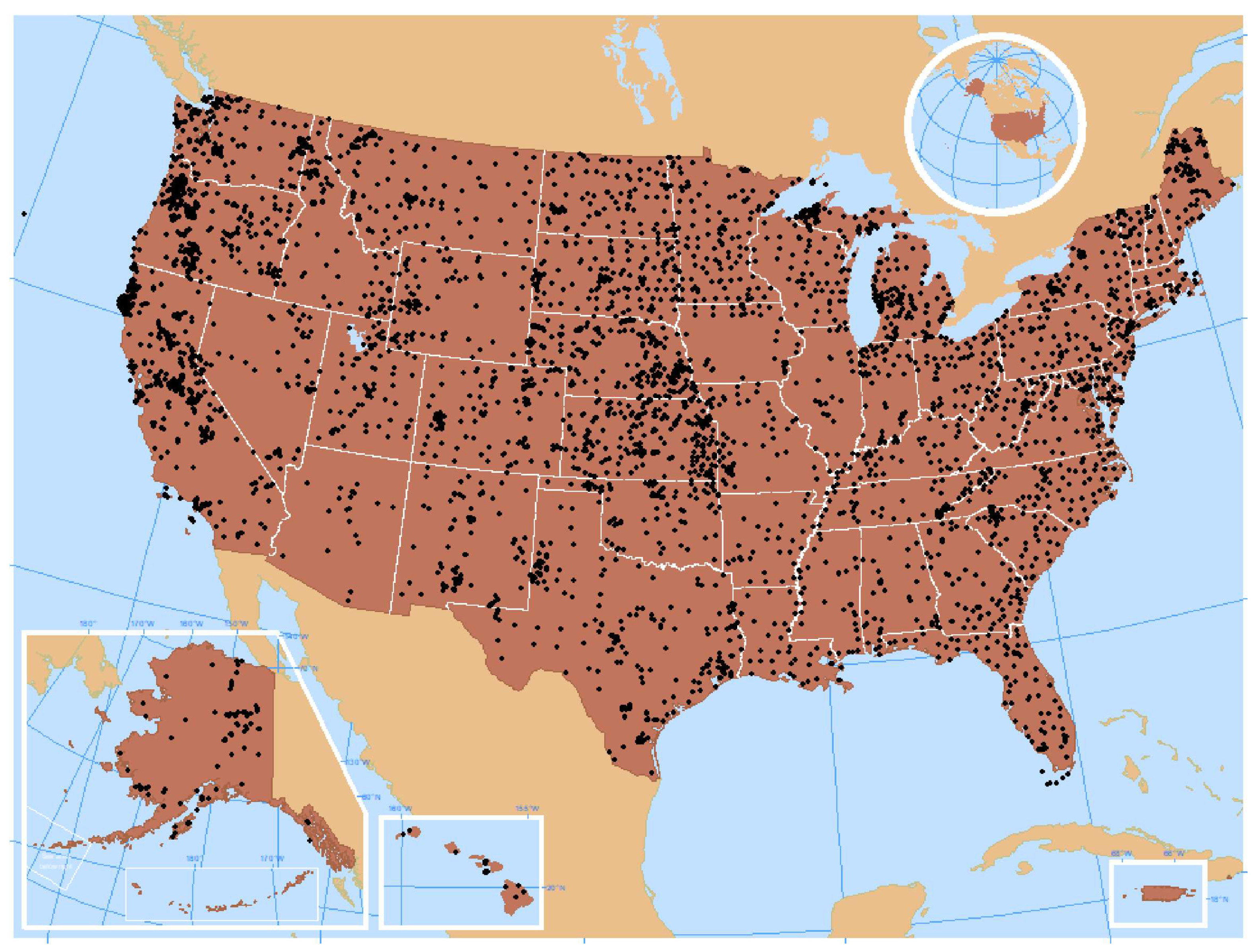
2.1. The NSSC-KSSL Spectral Library

The soil samples used in this study are extracted from the existing soil spectral library at the USDA NSSC-KSSL. While the current NSSC-KSSL soil characterization database contains >110,000 soil samples, the current (as of June 2018) MIR spectral library consists 15,118 pedons, representing 54,211 samples that have some associated analytical data (Figure 1). The 54,211 samples represent the wide range of land use and geologic conditions, allowing us to test several statistical approaches relevant to developing robust calibration models. All data are publicly available via request from the USDA National Soil Survey Center.

In this study, we focused on 10 soil physical and chemical properties, including organic carbon (OC, %), which was measured as total carbon by elemental analysis minus any inorganic carbon measured manometrically; calcium carbonate (CO₃, %) measured by manometer; cation exchange capacity (CEC, cmolc kg${}^{-1}$) and exchangeable calcium (Ca, cmolc kg${}^{-1}$) measured by displacement with ammonium oxalate, buffered at pH 7; clay (%) by sedimentation, pH in 1:1 water suspension; bulk density (BD, g/cm${}^{-3}$); dithionite citrate extractable aluminum (Al, %); acid oxalate extractable iron (Fe, %); and organic carbon density (OCD, kg m${}^{-3}$) calculated as the product of OC × BD × (1 − CF), where CF is coarse fragments (>2 mm) by volume. Detailed lab protocols can be found elsewhere [54].

The existing soil spectral library at the USDA NSSC-KSSL consists of BD data obtained with two different measurement techniques [55]: (1) clod and (2) core methods. The clod method involves extraction of an intact soil clod followed by the determination of the dry weight of the soil. The volume of the clod is measured after equilibration at 1/3 bar water tension. In contrast, the core method involves extracting soil samples using a known volume of a metal cylinder. The extracted samples are then oven-dried, sieved and weighed to determine the BD of the fine earth fraction. The clod has been the standard soil survey method but is only successful in soils with a fair degree of coherence; therefore, the method is biased away from sandy or organic-rich topsoils. In this study, we evaluated the models using clod, core and combined (clod and core together) methods.

The MIR spectra were acquired on air-dried and ground soil samples (to pass an 80-mesh sieve) using a Bruker Vertex 70 FTIR spectrometer with an HTS-XT high-throughput accessory. The sampling plate in the spectrometer consists of standardized 96-well microplates. On each 96-well microplate, 23 samples were prepared in quadruplicate, while the four remaining blank spots were used for reference readings. At each spot, 32 co-added scans were collected at a resolution of 4 cm${}^{-1}$. Both the sample MIR and reference scans are available in OPUS format, which was converted to text file for developing calibration models using an open-source programming platform [56].

2.2. Pre-Processing of MIR Spectra and Analytical Data

The four replicates of spectra corresponding to each sample were averaged to create a dataset containing both laboratory measurements of soil properties and MIR spectra. Spectra were truncated to 6000–600 cm${}^{-1}$, and regions showing atmospheric CO₂ features (2389–2268 cm${}^{-1}$), which are not associated with changes in soil samples [57], were removed. Spectra were then baseline corrected using the baseline-offset transformation before developing the calibration models. Since multivariate regression methods intrinsically require the data to be normally distributed, we assessed different transformation approaches prior to building multivariate PLSR models. We first chose two analytical data with normal (pH) and non-normal (OC) distributions. The normality of these two analytical data was explored by building histograms and calculating skewness and kurtosis (Figure S1 in Supplementary Materials). We then built PLSR models using box-cox-, square-root- and log-transformed and untransformed analytical data by dividing the data into calibration (80%) and validation (20%) sets to assess the prediction performance of near-normally distributed pH and non-normally distributed OC. On the basis of this analysis, we found that PLSR models built with square-root-transformed analytical data were, on average, superior (low RMSE and high R²) compared with box-cox-transformed and untransformed data, particularly when PLSR calibration models were applied to independent validation sets (Table S1; Figure S2). However, for other calibration methods (random forest, Cubist and MBL), none of these data transformations improved the prediction performance of pH and OC (Table S1). Although machine learning methods, such as random forest, Cubist and MBL, do not require the data to be normally distributed, for consistency, analytical data were square-root-transformed prior to developing calibration models using all methods (Figures S3 and S4).

2.3. Sample Selection, Outlier Detection and Model Performance Assessment

Large datasets invariably have erroneous data. Those errors can occur in both analytical and spectral data. Therefore, to detect outliers in the spectral library, we followed a two-step procedure. In the first step, we built PLSR models and tested their performance using all samples in the spectral library. Then, we defined a criterion to detect outliers based on the predictive performance of the model. In this study, outliers are defined as those sample points that fall outside a defined standard deviation threshold from the fitted (one-to-one) line. The standard deviation threshold was optimized such that it removed a maximum of 1% of the samples that fell beyond the threshold value in both the calibration and validation datasets (

Table 1. Summary statistics of soil properties available through the NSSC KSSL MIR library.

Soil	Units	Ntotal	Noutlier	Mean	Median	SD	Q25	Q75	Skew	Kurt
Al	wt %	23,121	229	0.19	0.10	0.32	0.04	0.21	8.52	143.13
BDclod	g cm${}^{-3}$	10,653	100	1.35	1.38	0.27	1.22	1.52	−1.05	5.34
BDcore	g cm${}^{-3}$	7071	68	0.93	1.01	0.50	0.51	1.30	0.21	7.94
BDall	g cm${}^{-3}$	17,488	173	1.18	1.29	0.43	1.00	1.47	−0.73	7.02
Ca	cmol(+) kg${}^{-1}$	36,854	368	23.09	12.30	34.43	3.69	28.65	4.15	28.18
CEC	cmol(+) kg${}^{-1}$	36,936	349	22.81	16.58	25.73	8.47	26.10	3.64	27.25
Clay	wt %	33,156	313	22.44	20.49	15.92	9.39	32.36	0.80	3.40
CO3	wt %	12205	120	6.92	1.00	12.05	0.21	9.24	2.98	14.73
Fe	wt %	21,530	212	0.44	0.26	0.63	0.10	0.57	8.84	191.11
OC	wt %	42,893	404	7.72	1.33	14.15	0.42	4.95	2.14	6.28
OCD	kg m${}^{-3}$	15,812	158	19.84	12.25	24.72	4.62	26.37	5.39	87.29
pH	NA	35,297	348	6.42	6.26	1.30	5.43	7.56	0.12	2.25

BD_clod and BD_core measure weight per unit volume of the <2 mm fraction, with volume measured after equilibration at 1/3 bar water tension in the case of the clod method and at field moisture in the case of the core method. BD_all combines information from both the clod and core method, providing a much wider range of bulk density estimates. In the case of carbonates (CO₃), we first built a random forest classification model to detect the presence/absence of CO₃ (N = 18,592) according to the results of a fizz test. Then, we removed outliers and built multivariate and machine learning models on samples that had detectable CO₃ (N = 12,205). Abbreviations—BD: bulk density; CEC: cation exchange capacity; OCD: organic carbon density.

; Figure S5). This method of detecting outliers is predicated upon being able to build reasonably reliable PLSR models but is superior to any method that focuses only on the spectral data.

In the case of CO₃, we first built a random forest classification model to detect the presence/absence of CO₃ according to results from a fizz test using 1 N HCl. Random forest performed better (out-of-bag error rate of 12%) in classifying the presence/absence of CO₃ (N = 12,205 for presence and N = 6387 for absence) than PLSR model. For further analysis, we only used samples that had detectable CO₃ according to the random forest output.

Following outlier detection, we divided the MIR spectral library into calibration and validation datasets using a Kennard Stone (KS) algorithm [58]. The KS algorithm is a deterministic approach that uses Euclidean or Mahalanobis distance to select a set of samples uniformly distributed in principal component (PC) space. Using the prospectr package in R, we selected 80% of the most representative samples in the library to calibrate the model. The remaining 20% of the samples were assigned to validation datasets to assess the predictive performance of the MIR models. The performance of the MIR models was assessed using bias, R², RMSE and RPD on independent validation sets (detailed in Section 2.5).

2.4. Spectral Modeling

2.4.1. Partial Least Squares Regression (PLSR)

Partial least squares regression (PLSR) is a multivariate regression technique widely used in chemometrics to study the relationship between highly collinear multi-dimensional predictor variables and a response variable. The PLSR algorithm follows a linear multivariate model that selects orthogonal (latent) factors to maximize the covariance between predictor (e.g., MIR data) and response (e.g., soil properties) variables [20,59]. As we deal with 2737 predictor variables for every response variable, the PLSR procedure helps to reduce the number of predictor (spectra) variables to a few independent variables that explain the most variation in the MIR spectra. In this study, global PLSR models were developed using the pls package [59], which decomposes the predictor (X) and the response (y) variables into scores (T) and loadings (P and q) as follows:

$$X=T{P}^{\prime }+E$$

(1)

$$y=Tq+f$$

(2)

where E and f are the residuals associated with the predictor and response variables, respectively. The final regression model used to predict soil properties is of the following form:

$$y_i={\beta }_0+{\beta }_1{t}_{1i}+{\beta }_2{t}_{2i}+\dots \dots \dots \dots \dots +{\beta }_n{t}_{ni}$$

(3)

where $\beta$₀ is the intercept of the global PLSR model; $\beta$₁, $\beta$₂ … $\beta$_n are the regression slopes for n latent variables (principal components); and t_1i, t_2i … t${}_{ni}$ are the scores from principal component 1 to n for response variable i.

In global PLSR, the optimal number of principal components (PC) to retain in the final model is determined using a one-sigma heuristic approach [60]. In this approach, the number of PCs corresponding to the initial best model (lowest RMSE) is determined using 10-fold cross-validation by examining models with up to 20 PCs. Then, the model with the fewest components that still falls within one standard error of the residuals (observed–predicted) of the overall best model is retained as the optimal number of PCs. This was accomplished using the selectNcomp function in pls package [59].

2.4.2. Memory-Based Learning (MBL)

Memory-based learning (i.e., local modeling) is a lazy learning approach in which, for each new target spectrum requiring a prediction of a given response variable, a new target function is fitted using a relatively small subset of spectrally similar samples found in a large reference set [24]. The spectrally similar samples (neighbors) can be found by using different similarity search methods, such as the Pearson’s correlation coefficient between spectra or Mahalanobis distances in the principal component (PC) space (or PC distances). Common methods to fit the local target functions include PLSR, Gaussian process [24] and weighted-average PLSR [61]. In this study, we used PLSR models to fit the local target functions, while neighbor searches were performed using Mahalanobis distances in the PC space. The number of PCs to retain was selected using an optimized principal component approach (oPC-M) [24]. MBL was conducted using the resemble package in R. Modifications to the MBL were made to output spectrally similar neighbors based on Euclidean distance in the PC space and provide uncertainty estimates of each new prediction.

2.4.3. Random Forest (RF)

Random forest is an ensemble machine learning technique that was developed as an extension of classification and regression trees (CART) to improve the prediction performance of the model [62]. The model-building process is the same as that for CART, where a recursive partitioning of the dataset is done to explore the relationship between the response and predictor variables [63]. Unlike CART, numerous trees are generated by using a subset of predictor variables, and all the responses are aggregated to get one single prediction. While generating each tree, a bootstrap sample (samples with a replacement) of the original data is selected, and the performance of each tree is validated using one-third of the samples that were not used for building that tree (out-of-bag error estimate). Random forest was implemented in R using the ranger package [64], where the number of trees to build is provided using the num.trees parameter. The number of trees can substantially affect the accuracy of the random forest model and depend on the number of response variables and predictor variables. When observations are sufficiently larger than the number of predictor variables, fewer trees are required and vice versa. For example, Hengl et al. [65] indicated that 150 trees are optimal to achieve a stable random forest model, beyond which a trade-off between the computation time and model accuracy offers no additional benefits. Given that the number of response variables is much larger than the number of predictor variables, we used 150 trees as a compromise between accuracy and computational time in this study.

2.4.4. Cubist

Cubist is a machine learning algorithm that constructs model trees using the CART approach [63], with linear models at each terminal nodes [66]. Unlike other decision trees (for example, random forest) that retrieve the final model on the basis of discrete values, Cubist uses a set of multivariate models associated with a set of rules at each terminal node. The final prediction is based on the linear model that satisfies the set of conditions associated with the predictor variables [67]. The splitting criteria are also slightly different between CART and Cubist, with CART using the variance and Cubist using the standard deviation as a measure of error [68]. The Cubist model was implemented in R using the Cubist package [67], which is an extension of Quinlan’s M5 model tree. Cubist requires setting up a committees parameter, where iterative model trees are created in sequence according to the number of committees using a boosting-like scheme. However, as a compromise between accuracy and the computational time required to run the Cubist, we did not implement the boosting-like algorithm, and we set the number of committees to 1 during the course of this study.

2.5. Assessment of Model and Individual Prediction Performance

2.5.1. Model Performance

In this study, we assessed the overall accuracy and precision of each model using the coefficient of determination (R²), ratio of performance to deviation (RPD), root-mean-square error (RMSE) and model bias. The R², RPD, RMSE and bias were computed for each property and each modeling approach according to the following equations:

$$RMSE=\sqrt{\frac{1}{n}\sum _{i=1}^n{(y_i-{\widehat{y}}_i)}^2}$$

(4)

$$RPD=\frac{\sigma }{RMSE}$$

(5)

$$bias=\frac{1}{n}\sum _{i=1}^n(y_i-{\widehat{y}}_i)$$

(6)

where $yi$ is the observed value of the ith sample measured by conventional laboratory methods, ŷ_i is the predicted value of the ith sample, n is the number of samples and $\sigma$ is the standard deviation of the observed soil property in the calibration or validation set.

We further defined criteria to assess the relative fit of the model using RPD: (1) RPD ≥ 2.0 (excellent models); (2) 1.4 ≤ RPD < 2 (fair models); and (3) RPD < 1.4 (non-reliable models) [69]. However, it is important to note that the criteria to define excellent and poor models using RPD are rather arbitrary, and there is no statistical basis on how these classification thresholds are determined [70]. We feel it is more important that a user evaluates model performance with respect to the objective of the study.

2.5.2. Individual Prediction Uncertainty

In addition to overall model performance, characterizing the prediction uncertainty of each sample is crucial in order to know the quality or reliability of each new prediction when relying purely on spectral-based predictions [70]. Therefore, we estimated the uncertainty associated with each new prediction in the validation sets using two different approaches. In the case of the PLSR and MBL models, we used the U-deviation method, as implemented in the Unscrambler software package (CAMO) and subsequently improved by De Vries and Ter Braak [50]. The U-deviation method is an empirically derived formula that takes into account the residual variance in the validation sets and the error in the product of scores and loadings [50]. Mathematically, PLSR and MBL make new predictions using the following relationship:

$$y_{pred,i}=y_{cal}+t_{pred,i}\times q^T$$

(7)

where $t_{pred,i}$ is the score for predicted sample i, and $q^T$ is the y-loadings from the calibration set. Thus, U-deviation can be estimated from the error in y-mean and the error in the product of score and loadings. The final equation for estimating U-deviation is as follows:

$${\sigma }_{pred,i}=\sqrt{{\sigma }_{valid}\times (1-\frac{A+1}{n})\times (h_0+\frac{{\sigma }_X}{{\sigma }_{X,valid}}+\frac{1}{n})}$$

(8)

where ${\sigma }_{valid}$ is the y-residual variance in the validation set, ${\sigma }_X$ is the x-residual variance in the calibration set, ${\sigma }_{X,valid}$ is the average x-residual variance in the validation set, $H_0$ is the leverage of the prediction sample and can be seen as the distance of each sample in the validation sets to all the samples in the calibration set, A is the number of principal components used to build the model and n is the number of samples in the validation set.

In the case of random forest, we used the infinitesimal jackknife to provide the standard error associated with each new prediction in the validation datasets. The general approach of the jackknife follows a resampling technique whereby prediction is computed by omitting one observation at a time. These individual predictions are then combined to provide an estimate of the variance or bias correction [71,72]. In contrast, rather than remove one observation at a time, the infinitesimal jackknife approach assigns a weight to each observation to provide the estimate variance [73]. The infinitesimal jackknife approach has been considered to give more stable predictions compared with the jackknife approach [72]. Therefore, we used the infinitesimal jackknife approach to provide uncertainty estimates of each new prediction using the ranger package [56]. Unfortunately, assessing the prediction uncertainty in the Cubist model using a jackknife or other bootstrapping approach is currently computationally prohibitive with the large datasets used in this study.

Although the model uncertainty was estimated for all soil properties and summarized as the mean deviation of the validation set, we only show detailed uncertainty estimates for two soil properties (OC and BD) using the validation sets. These two soil properties were selected on the basis of the best (OC) and worst (BD) model performance in the validation sets using the local PLSR model.

2.5.3. Trustworthiness of New Predictions

Individual prediction uncertainty estimates were also used to assess the trustworthiness of new predictions. When an MIR-based prediction model is used independently of laboratory data, there must be a way of flagging when predictions should not be trusted because the new sample falls outside of the calibration space [74]. To determine the trustworthiness of the predicted soil property using PLSR and MBL models, we first determined the outliers in the spectra using F-ratios (F) [75]:

$$F_i=\frac{(M-1){\left({ϵ}_i\right)}^2}{{\sum }_{j\ne i}{\left({ϵ}_j\right)}^2}$$

(9)

where M is the number of samples in the calibration set, ${ϵ}_i$ denotes the spectral residuals for the ith sample in the calibration sets and ${ϵ}_j$ denotes the spectral residuals of all samples in the calibration set with the ith sample excluded.

The F-ratio and M − 1 degrees of freedom are used to derive the probability distribution such that spectra with a probability of greater than 0.99 are flagged as an outlier in the analysis:

$$F_{prob(F,1,M-1)}>0.99$$

(10)

In the case of the PLSR model, a prediction was considered unreliable if the spectra fell outside the calibration space with an F-ratio greater than 0.99. However, since MBL uses spectrally similar neighbors to make predictions for new samples, we defined an additional criterion to detect samples yielding unreliable predictions. New predictions were considered unreliable if the new sample used spectrally similar neighbors with an F-ratio greater than 0.99 to make the prediction. Since the RF model uses a different approach to make predictions and does not rely on the relative location of spectra in orthogonal space, we detected outliers using the probability distribution of the relative deviation (uncertainty/predicted value) from the validation sets. Samples were flagged as untrustworthy when the probability of the relative deviation was greater than 0.99.

Data processing, analysis and prediction were carried out using high-performance Google Cloud computing (https://cloud.google.com) with 52 GB RAM, Google bucket unlimited hard disk space and 8 cores running on a Debian GNU/Linux 9 operating system and R 3.2.3 platform. Multiple VM instances were created in Google Cloud to speed up data processing, analysis and prediction. Total computational time from scratch was approximately 121 CPU hours. The script used for processing, analysis and prediction of all soil properties is freely available in the WHRC GitHub (https://github.com/whrc).

3. Results

3.1. Exploratory Analysis of the KSSL MIR Library

Many of the soil properties in this study deviate substantially from the normal distribution, as indicated by their high skewness values (a measure of symmetry) and kurtosis (a measure of heavy or light tail relative to the normal distribution) (Table 1). Clay content, bulk density and pH appear to be normally distributed, as their skewness values are close to 0, and their kurtosis values are close to 3. On the other hand, CO₃, CEC, exchangeable Ca and the extractable phases of Al and Fe are skewed and heavily tailed, indicating a non-normal distribution. Across different soil horizons, OC was found to be the highest in the O horizon with a mean value of 35.7 wt %, while carbonates (CO₃) were the highest in the B, B/C and C horizons with mean values of 7.8, 8.5 and 9.2 wt %, respectively. While half of the samples did not have a recorded soil order, all soil orders except oxisols (n = 6) and gelisols (n = 214) are represented by >500 samples (

Table 2. Distribution of samples in the NSSC KSSL MIR library as a function of soil order and horizon.

Soil Horizons
Order	O	A	E	B	C	R	Undefined	Total
Alfisols	65	727	195	1918	216	1	289	3411
Andisols	157	368	13	616	116	2	20	1292
Aridsols	0	222	4	674	155	0	46	1101
Entisols	52	380	61	238	631	0	289	1651
Gelisols	72	13	0	32	59	0	38	214
Histosols	507	9	4	10	114	0	80	724
Inceptisols	191	729	42	1229	618	4	332	3145
Mollisols	47	2571	59	3608	823	0	1010	8118
Oxisols	0	1	0	5	0	0	0	6
Spodosols	129	116	212	744	221	1	20	1443
Ultisols	55	409	85	1002	130	0	235	1916
Vertisols	0	72	1	275	37	0	133	518
Undefined	514	1023	58	1243	371	0	24,145	27,354
Total	1789	6640	734	11,594	3491	8	26,637	50,893

).

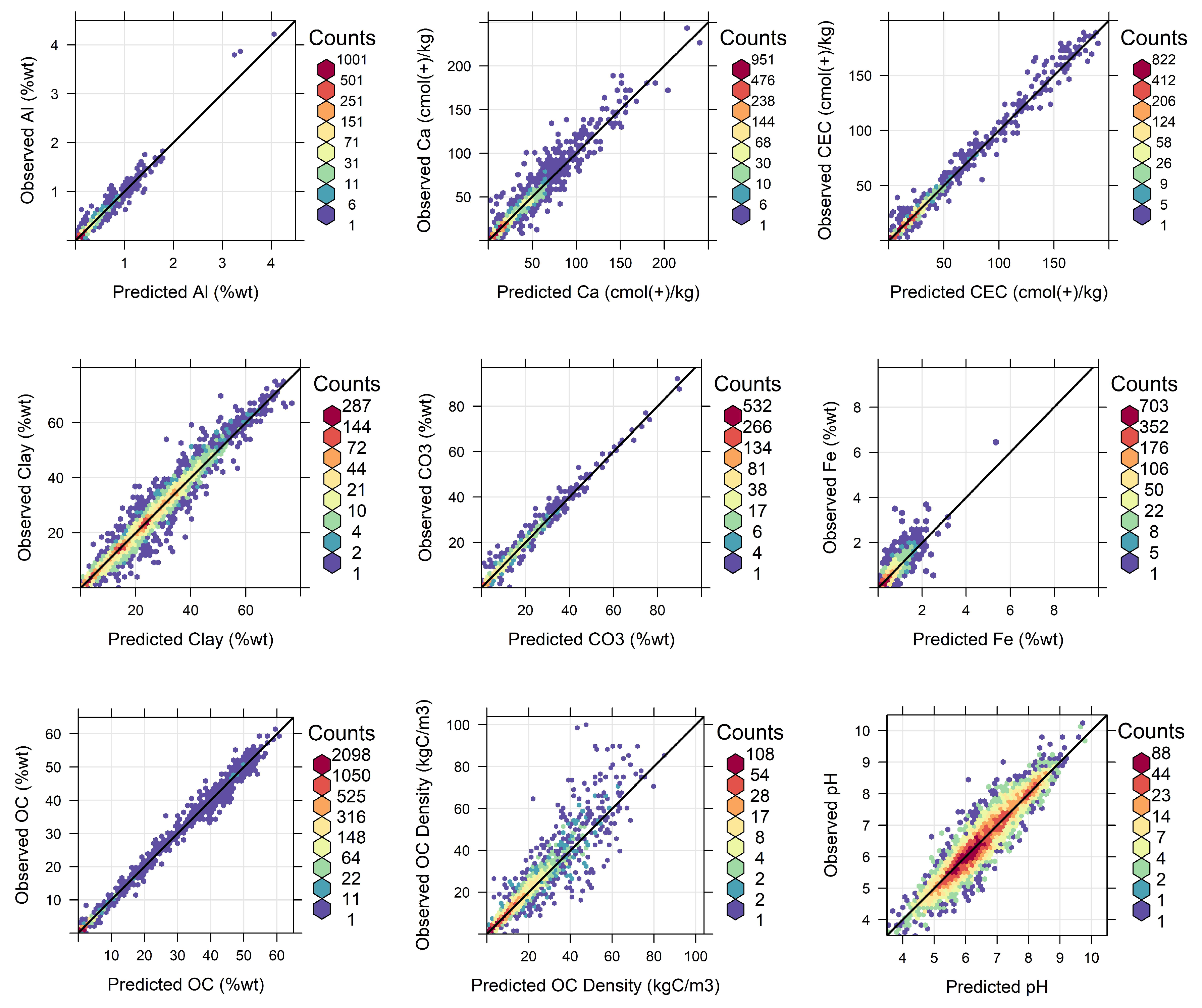
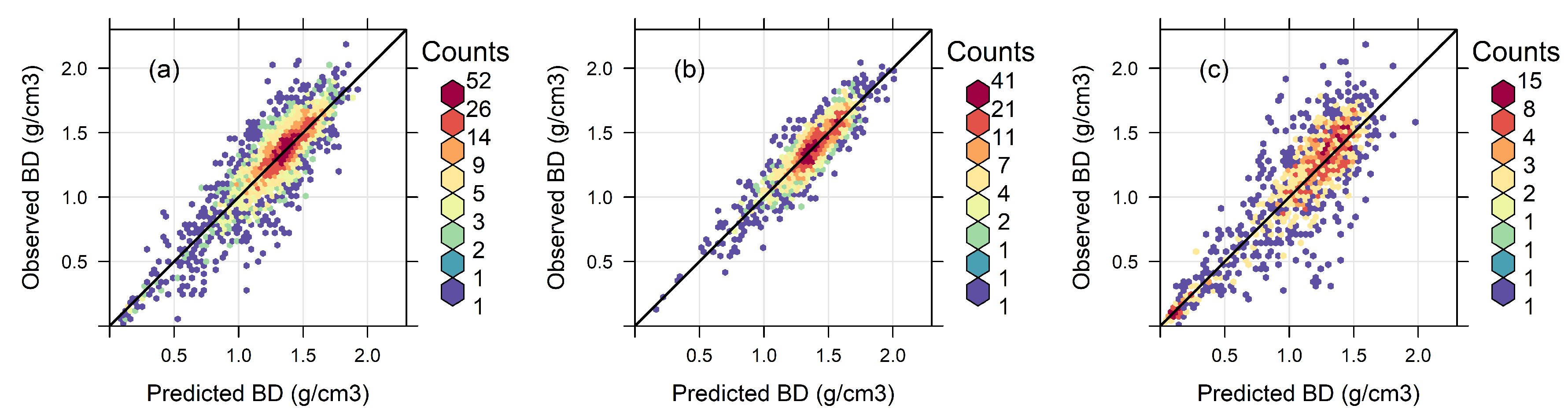
3.2. Overall Model Performance

Results show that excellent calibration models were obtained with RPD ≥ 2.0 for all soil properties using the Cubist and RF models (

Table 3. Calibration and validation results of nine soil properties using partial least squares regression (PLSR) and machine learning (memory-based learner (MBL), Cubist and random forest (RF)) models.

Soil Property	Method	Calibration					Validation
		N	Bias	R2	RPD	RMSE	N	Bias	R2	RPD	RMSE	MeanDev
OC	Cubist	33,991	0	1.0	16.9	0.85	8498	0.01	1.0	16.9	0.69
	MBL							0.03	1.0	18.2	0.64	0.08
	PLSR		0.05	0.98	8.0	1.8		0.12	0.99	9.8	1.19	0.26
	RF		0.05	1.0	20.7	0.69		0.11	0.99	12.5	0.93	0.39
CO3	Cubist	9668	0.04	0.99	11.1	1.18	2417	−0.01	0.98	8.0	1.35
	MBL							0.14	0.98	7.6	1.41	0.33
	PLSR		0.09	0.97	6.1	2.17		0.04	0.97	5.9	1.81	0.70
	RF		0.17	1.0	15.3	0.86		0.36	0.97	5.9	1.82	0.64
CEC	Cubist	29,270	0.16	0.98	7.3	3.45	7317	0.24	0.99	8.3	2.38
	MBL							0.07	0.99	8.6	2.3	0.33
	PLSR		0.25	0.94	4.1	6.1		0.45	0.96	4.9	4.02	1.38
	RF		0.26	0.99	10.2	2.48		0.51	0.97	5.8	3.44	1.52
Clay	Cubist	26,274	0.07	0.97	5.5	2.92	6569	0	0.96	5.1	2.69
	MBL							0.03	0.97	5.5	2.47	0.41
	PLSR		0.34	0.89	3.0	5.43		−0.24	0.92	3.5	3.95	1.86
	RF		0.41	0.98	7.2	2.25		0.2	0.93	3.8	3.57	3.79
Ca	Cubist	29,189	0.34	0.96	5.2	5.65	7297	0.27	0.95	4.7	4.41
	MBL							0.12	0.95	4.6	4.49	0.47
	PLSR		0.68	0.86	2.7	10.79		0.64	0.89	3.0	6.85	2.07
	RF		0.69	0.98	7.2	4.03		0.67	0.93	3.8	5.43	4.06
Al	Cubist	18,314	0	0.95	4.7	0.05	4578	0	0.9	3.1	0.08
	MBL							0	0.97	5.4	0.04	0.01
	PLSR		0.01	0.83	2.5	0.1		0.01	0.85	2.6	0.09	0.03
	RF		0.01	0.97	5.9	0.04		0.02	0.83	2.4	0.1	0.03
OCD	Cubist	12,523	0.42	0.89	3	6.2	3131	0.39	0.89	3.0	5.23
	MBL							0.95	0.89	3.0	5.17	0.61
	PLSR		0.49	0.82	2.3	8.09		1.19	0.86	2.6	5.93	1.96
	RF		0.42	0.97	6.0	3.13		0.8	0.87	2.8	5.6	1.66
pH	Cubist	27,959	0	0.95	4.4	0.31	6990	0.01	0.88	2.9	0.36
	MBL							0	0.89	3.1	0.34	0.05
	PLSR		0.01	0.8	2.3	0.59		0.04	0.74	1.9	0.54	0.27
	RF		0.01	0.98	6.4	0.21		0	0.82	2.4	0.45	0.21
Fe	Cubist	17,054	0.02	0.88	2.9	0.18	4264	0.01	0.71	1.9	0.27
	MBL							0.02	0.81	2.3	0.22	0.02
	PLSR		0.04	0.58	1.5	0.34		0.03	0.66	1.7	0.29	0.09
	RF		0.03	0.95	4.4	0.12		0.04	0.69	1.8	0.28	0.06

Ratio of performance to deviation (RPD) is calculated as the ratio of standard deviation of the observed soil property to the root-mean-square error in the prediction, and mean deviation (MeanDev) is the average of the uncertainty estimates for all samples in the validation sets. All predictions were back-transformed prior to calculating goodness-of-fit statistics.

). Global PLSR also produced excellent calibration models for all soil properties except Fe (fair model; RPD = 1.5). When the performance of the calibration models was assessed using R², RF produced calibration models with R² ≥ 0.95 for all properties. Cubist also produced calibration models with R² ≥ 0.95 for all properties except Fe (R² = 0.88) and BD (R² = 0.88, 0.87 and 0.88 using clod, core and combined clod and core approaches, respectively). The global PLSR models produced calibration models with R² ≥ 0.94 for OC, CO₃ and CEC, while it had slightly lower R² for clay, OCD, Ca, Al, pH and BD (using core and combined approach) (0.80 ≤R²< 0.90). The calibration models with the lowest R² were obtained for BD (R² = 0.77 using the clod approach) and Fe (R² = 0.58), respectively. The optimal number of principal components selected in the global PLSR models using the one-sigma approach was 20 for all soil properties except BD, for which 19 and 16 components were selected for the clod and core methods, respectively, and 18 components were used for the combined BD model. Since MBL produces new calibration models for the prediction of each sample, there are no calibration statistics for the local model.

When these models were tested on an independent validation set, MBL (Figure 2) demonstrated excellent performance, with RPD ≥ 2.0 for all soil properties. Cubist (Figure S6) and RF (Figure S7) also showed excellent model performance, with RPD ≥ 2.0 for all soil properties except Fe and BD using the combined clod and core methods (fair models; 1.7 ≤ RPD ≤ 1.9). The global PLSR (Figure S8) produced fair models when tested on an independent validation set for pH (RPD = 1.9), Fe (RPD = 1.7) and BD using the clod-only and combined clod and core methods (RPD = 1.8 and 1.7, respectively). When model R² was used to test the predictive performance of all models, Cubist (Figure S6) and MBL (Figure 2) predicted all soil properties with R² ≥ 0.90 except OCD, pH, Fe and BD (Table 3 and

Table 4. Calibration and validation results of soil bulk density using PLSR and machine learning (memory-based learner (MBL), Cubist and random forest (RF)) models. Prediction of soil bulk density was assessed by fitting the model using data from two analytical methods (clod—volume measured at 1/3 bar water tension and core—volume measured at field soil moisture condition) and the two analytical methods combined (BD_all). All predictions were back-transformed prior to calculating goodness-of-fit statistics.

Soil Property	Method	Calibration					Validation
		N	Bias	R2	RPD	RMSE	N	Bias	R2	RPD	RMSE	MeanDev
BDclod	Cubist	8442	0	0.88	2.9	0.1	2111	−0.01	0.75	2.0	0.11
	MBL							0	0.81	2.3	0.1	0.01
	PLSR		0	0.77	2.1	0.14		0.01	0.71	1.8	0.12	0.05
	RF		0	0.97	5.7	0.05		0	0.78	2.1	0.1	0.04
BDcore	Cubist	5602	0	0.87	2.8	0.17	1401	0.02	0.78	2.1	0.21
	MBL							0.02	0.79	2.2	0.21	0.02
	PLSR		0.01	0.82	2.4	0.21		0.06	0.77	2.1	0.22	0.1
	RF		0.01	0.97	5.9	0.08		0.05	0.79	2.2	0.21	0.06
BDall	Cubist	13,852	0	0.88	2.9	0.16	3463	0	0.67	1.8	0.16
	MBL							0.01	0.76	2.0	0.14	0.02
	PLSR		0.01	0.81	2.3	0.19		0.02	0.64	1.7	0.17	0.08
	RF		0.01	0.97	6.0	0.07		0.03	0.72	1.9	0.15	0.08

). The random forest models (Figure S7) showed the greatest drop in performance between calibration and validation sets, with R² values dropping by 0.16 and 0.26 for the more difficult to predict properties (pH and Fe, respectively). In the case of BD, model fit (R²) dropped by 0.19, 0.18 and 0.25 using the random forest models (clod, core and combined approaches, respectively). Cubist also demonstrated a tendency to overfit for these three properties (pH, Fe and BD using all three methods). On the other hand, the global PLSR models (Figure S8) held up to the independent validation data and produced very similar performance statistics (Table 3 and Table 4). For the properties with the best predictions (OC, CO₃, CEC and clay)—i.e., properties for which all models produced R² > 0.92—the RMSE values suggested that MBL outperformed the Cubist, PLSR and RF models. The RMSE values for RF and PLSR were 35–86% higher, while those of Cubist were 3–9% higher than the RMSE values for MBL for the top four properties (with R² > 0.92). For other soil properties, such as Ca, Al, pH and Fe, the RMSE values for the RF and PLSR models were 23–150% higher than the RMSE values using the MBL and Cubist models.

For bulk density, which is a more difficult to predict soil property, evaluation of model performance on independent validation sets indicated that MBL (Figure 3) and RF (Figure S9) were slightly superior compared with the Cubist and PLSR models (RMSE improved by 7–21%) using combined samples (clod and core) (Table 2 and Table 3). However, the MBL, Cubist and RF models showed a similar performance (RMSE = 0.21) in the case of BD estimated using the core method. For BD estimated using the clod method, MBL and RF slightly outperformed the Cubist and PLSR models (10–20% improvement in RMSE).

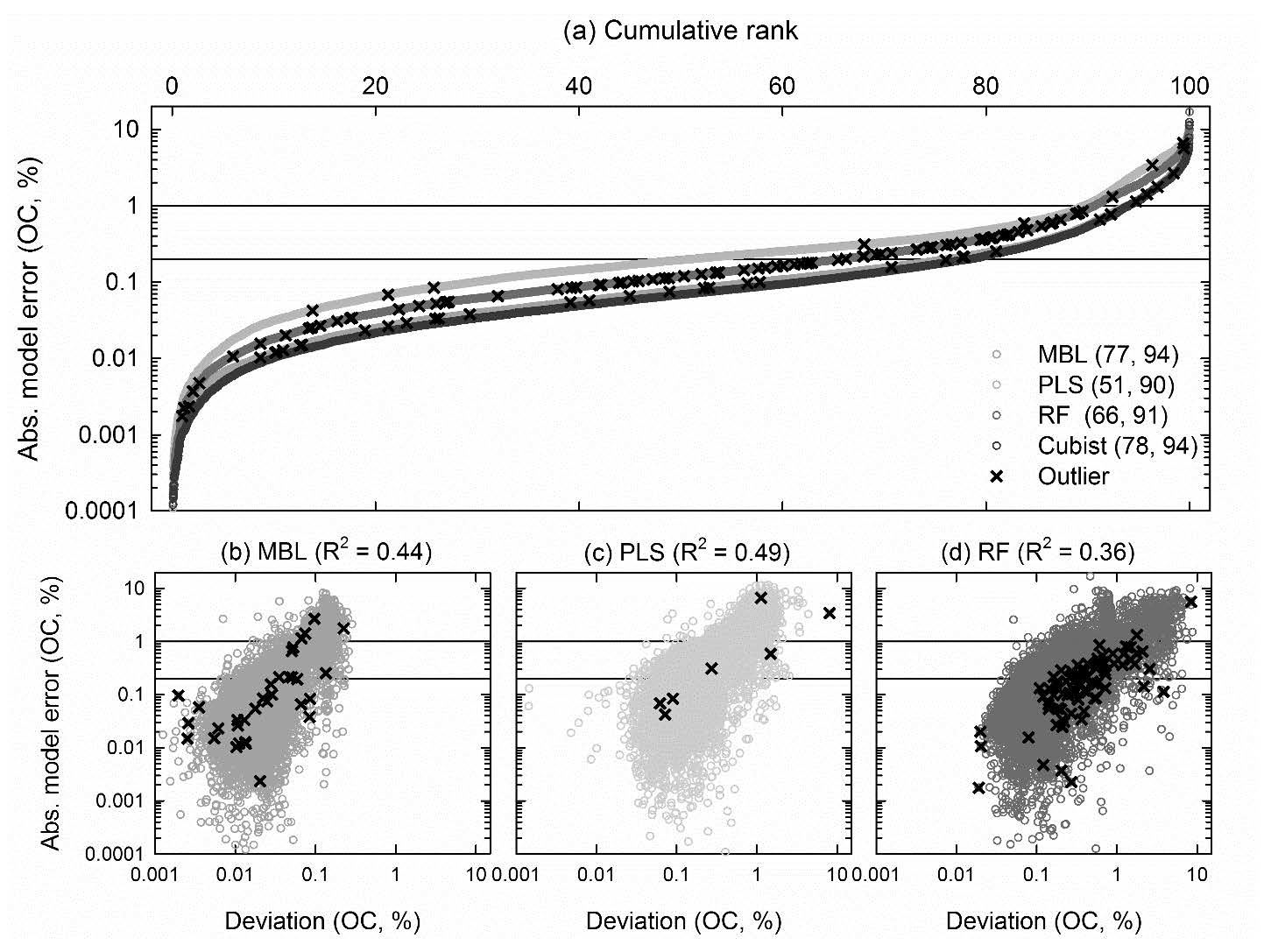
3.3. Absolute Model Error and Prediction Uncertainty

While the RPD, R² and RMSE values give an indication of overall model performance, examination of the absolute error (observed–predicted values) in the validation sets is particularly diagnostic. A comparison of absolute model error for OC shows that MBL predicted 77% and 94% of the samples, with absolute model error ≥ 0.2 wt % and ≥ 1.0 wt %, respectively (Figure 4a). Cubist produced very similar results, with 79 and 94% of the samples below the two thresholds. In the case of poorly predicted BD, MBL was still the superior model, predicting 58% and 85% of the samples with absolute model error ≥ 0.1 g/cm³ and ≥ 0.2 g/cm³, but was comparable to the absolute model error based on Cubist and RF (Figure S10). Despite an R² > 0.98 for the OC validation set using MBL and Cubist, about 6% of these samples were still predicted with poor accuracy (defined as absolute error > 1.0%). Figure S11 illustrates that these poor predictions can occur for almost any measured value of OC, but the relative error (model error/observed) was generally much lower for higher values.

Assessment of the prediction uncertainty for these soil properties indicated that the MBL model consistently provided a low prediction error compared with the PLSR and RF models. The mean prediction ± prediction error for OC in the independent validation sets was 5.17 ± 0.08, 5.06 ± 0.26 and 5.07 ± 0.39 (wt %) using the MBL, PLSR and RF models, respectively. Likewise, in the case of BD, mean prediction ± prediction error was 1.30 ± 0.02, 1.30 ± 0.08, 1.29 ± 0.08 (g/cm³) using the MBL, PLSR and RF models, respectively. Overall, our results show that the uncertainty estimates for OC using MBL (observed mean = 5.18 wt %) and BD (observed mean = 1.32 g/cm³) were within 1.5% and 2.3% of the predicted mean (5.17 wt % for OC and 1.3 g/cm³ for BD), respectively. Unfortunately, there is currently no method to assess the prediction uncertainty in Cubist. In the case of MBL, we further determined the samples with the highest and lowest prediction error for OC from the independent validation sets (N = 8498). The largest prediction error in the local model was often associated with picking neighboring samples that are farther apart in orthogonal space (Figure S12). For example, results show that the average distance between the neighbors and the prediction sample was 0.15 units for the sample with the largest prediction error. In contrast, the average distance in the case of the prediction sample with least prediction error was 0.10 units, indicating that prediction errors are low when samples that are spectrally similar are used to make predictions of any new samples.

We also assessed the trustworthiness of each new prediction in the validation sets by detecting outliers using the probability distribution of the relative deviation for RF and F-ratio (Equations (9) and (10)) for the MBL and PLSR models. The RF model flagged 86 samples, while the MBL and PLSR models flagged 33 and 7 samples, respectively, out of 8512 samples in the validation sets for OC (Figure 4 and Figure S13). In the case of BD, the RF model flagged 34 samples, while the MBL and PLSR models flagged 33 and 10 samples, respectively, out of 3306 samples in the validation sets (Figures S10 and S13). The samples flagged as having been unreliably predicted were distributed across the entire distribution of the absolute error and prediction uncertainty (Figure 4 and Figure S10), indicating that poorly predicted samples (high absolute error) were not flagged as outliers and did not have large prediction errors using all three models. Additionally, results show that the absolute error was significantly related to prediction uncertainty for OC but not for BD (Figure 4 and Figure S10).

4. Discussion

4.1. KSSL MIR Library and Its Non-Normal Distribution

In this study, we utilized a large nationally comprehensive soil MIR library (Figure 1) available through the USDA NSSC-KSSL soil database, which contains 15,118 unique pedons representing 50,893 samples with varying amounts of associated analytical data. As emphasized by Wijewardane et al. [16], the soil properties in the database mostly follow a non-normal distribution (Table 1). One way to improve the prediction of soil properties with data that follow a non-normal distribution is to transform the data using a variety of approaches, such as box-cox, natural log and square root transformation [8,11,30,45,76,77]. For example, Waruru et al. [77] applied natural log and square root transformation to highly skewed and slightly skewed soil properties, respectively. Baldock et al. [11] showed that square-root-transformed OC performed better than log-transformed OC by improving R² and reducing the model bias in both the calibration and validation sets. In this study, since some soil properties were highly skewed compared with others, we developed calibration models and tested their performance on independent validation sets using three different transformations (square root, box-cox and log) for two soil properties representing high skewness (OC) and near-normal distribution (pH) (Figures S1 and S2). The results from this exercise indicate that, for skewed data (OC), square root transformation produced the best PLSR model performance. For normally distributed data (pH), there was no improvement in performance. Additionally, for the machine learning (RF and Cubist) and local models (MBL), transformation was not necessary (Table S1).

4.2. Model Performance for a Range of Soil Properties

Our results indicate that MIR spectroscopy combined with a highly heterogeneous database can provide excellent predictions of most soil properties, with validation RPD ≥ 2.0, using both machine learning and regression approaches (Table 3 and Table 4). Only a few soil properties have RPD < 2.0 using the Cubist, RF and global PLSR models (Fe and BD_all for Cubist and RF models; Fe, BD_core and BD_all for PLSR model). Using R² to assess the prediction performance also produced similar results, with validation R² ≥ 0.98 for OC and CO₃ and validation R² ≥ 0.83 for CEC, clay, OCD, Ca and Al, regardless of the methodology used to develop the calibration models. For pH, Fe and BD (particularly for the clod and combined methods), the model choice made a significant difference in the quality of predictions (Table 3 and Table 4). Better prediction results were attributed particularly to strong absorption bands associated with soil mineral and organic bonds in the MIR region [6,7]. Additionally, due to the large spatial variation in soil properties, the relationship between spectra and soil attributes can be complex, requiring a large sample size to adequately represent the distribution of samples across space [5]. Models built using a large spectral database can help to minimize calibration errors and better predict soil attributes from independent datasets [45]. However, only a few large-scale vis–NIR databases and even fewer MIR libraries are available [78]. In addition, these spectral libraries have rarely been considered as an operational tool for the assessment and prediction of soil properties [10].

When the entire spectral library was used to build a single global model (global PLSR), soil properties such as OC and CO₃ were accurately predicted with an R² ≥ 0.98 (Table 3). Other studies using an MIR library to build global PLSR models have reported similar results for these properties. Baldock et al. [11] found a good prediction of OC (R² = 0.93) and CO₃ (R² = 0.93) in Australian soils. Similarly, McCarty et al. [15] reported a better prediction of OC (R² = 0.82) and CO₃ (R² = 0.87) using 273 samples from diverse locations in the central United States, while Grinand et al. [79] predicted OC with an R² of 0.89 and CO₃ with an R² of 0.97 in European soils using >1700 samples. The better PLSR performance in this current study in the prediction of OC and CO₃ is likely associated with the number of samples used to build the calibration models [25]. For example, using 10 different calibration intensities (from 10 to 100%), Clairotte et al. [25] found that the standard error of the validation samples decreased when the size of samples used to build the calibration model increased from 10 to 100%. Given the size of the MIR library used in this study, it is not surprising that the calibration models performed better when predicting OC and CO₃ compared with previous studies.

Assessment of the models on the basis of RMSE values presents a more nuanced picture, with greater discrepancies between different models (Table 3). While OC in an independent validation set was predicted with an R² of 0.99 by all models, the RMSE was 80% higher for the global PLSR model compared with Cubist and MBL. This increase in RMSE for the global model is most likely attributed to the fact that, for the prediction of any particular sample, there is a lot of extraneous information (i.e., samples with highly dissimilar properties) contained in the global PLSR model [76]. MBL, a nonlinear modeling approach, was designed to handle this exact problem [24] and had lower RMSE values for all properties compared with the global PLSR (Table S3). The superior performance of local PLSR compared with global PLSR is a result of local PLSR searching for spectrally similar neighbors in the PC space [24,80], thereby allowing the effective removal of uninformative and less relevant samples for each new prediction in the large spectral library. Using local regression, previous studies have found typically better prediction compared with global PLSR [24,25], although this is not always the case [26]. For example, the addition of new samples improved the prediction performance of CO₃ but led to the inaccurate prediction of other soil properties [26]. The improved model performance of CO₃ was due to the addition of new samples that were rich in carbonates.

Machine learning models can also handle this extraneous (nonlinear) information shortcoming in global PLSR models by finding patterns in the spectral library and sub-setting the data accordingly [37]. The Cubist and RF models generally outperformed the global PLSR models. Cubist consistently produced better prediction results with higher fitting R² and lower RMSE than RF for all soil properties except BD. Previous studies have demonstrated that the Cubist modeling approach is slightly superior in the prediction of soil properties compared with other machine learning approaches, such as support vector machines [10]. This is because Cubist is a form of piecewise linear decision trees that are able to make very efficient spectral variable selections and handle nonlinear relationships between dependent and independent variables [81]. The Cubist model constructs a regression tree in which each terminal node contains multivariate linear models instead of discrete values. The prediction of a soil property of a new sample is achieved first by identifying where the sample falls in the tree node, and then a linear model is fitted using all combinations of the samples within that node [82]. However, several studies have demonstrated that calibration models developed using Cubist tend to show a good model fit at low values, while the residuals increase at higher values [38,66]. Doetterl et al. [66] suggested that large residuals at high values are not a general feature of Cubist but are associated with a limited sampling density at high concentration values. In this study, we did not find any large residuals at higher values for all soil properties, which is possibly related to the inclusion of enough samples with high values. Interestingly, RF developed superior calibration models for all soil properties compared with Cubist, but the application of the calibration models to independent validation sets resulted in a significant decrease in performance compared with the Cubist model. This might possibly be associated with more continuous predicted values in the case of the Cubist algorithm, because each linear model at the terminal node in Cubist allows for a smoother transition in the prediction between trees [67]. However, in RF, a random subset of training data are selected through bagging, and the final prediction is the average of all individual tree outputs [62].

4.3. The Importance of Estimating Prediction Uncertainty

While the RMSE values reported in Table 3 give an indication of the overall model performance over a large range of each soil property (Table S3), those RMSE values do not give an indication of the uncertainty in individual predictions [68]. For example, all models produced excellent fits for OC (R² = 0.99), but the RMSE values were 0.70–1.27 wt %, which would be considered unacceptably high for most management applications. Therefore, we used approaches to provide uncertainty estimates for each prediction using the global PLSR, MBL and RF models. Here, there is a clear difference in model performance, with MBL producing significantly narrower prediction intervals compared with global PLSR and RF (Table 3, Figure 4).

Both the MBL and PLSR models use a similar approach to uncertainty estimation, but the models using MBL yielded a much narrower range of uncertainty estimates. This is because MBL searches for the most spectrally similar neighbors corresponding to each new prediction sample in the spectral library, thus introducing low residual variance to the calibration subset. The U-deviation uses four major parameters to estimate the prediction uncertainty: (1) x-residuals in the calibration set; (2) x-residuals in the validation set; (3) y-residuals in the validation set; and (4) the average distance of the validation samples to all the samples in the calibration sets used to make predictions [50]. Of the four parameters, the y-residuals in the validation set are the most difficult to estimate in the case of MBL, because this model uses different calibration subsets for predicting samples in the validation sets. As a result, the y-residual variance was estimated using a leave-group-out cross-validation. In the case of global PLSR, estimating the prediction uncertainty using U-deviation is fairly simple, because there is only one single model to make predictions for all samples in the validation sets. Therefore, y-residual variance is simply the variance in the response variable of the validation sets.

Prediction uncertainty using RF was higher than the global PLSR for OC but similar to the PLSR model for BD (Figure 2 and Figure 3). This difference may be due to the use of a different approach to estimating the prediction uncertainty. In the case of RF, we used the non-parametric infinitesimal jackknife approach, which is a modified jackknife approach [72]. In the jackknife approach, each observation is omitted to recompute the prediction of the remaining observations. This process is repeated for all the observations to produce an estimate of the variance. In the infinitesimal jackknife approach, rather than omitting one observation at a time, the observation is given a slightly lower weight compared with the other observations. Compared with the global PLSR and MBL uncertainty estimates, the infinitesimal jackknife approach relies more on the variance between the prediction and the observation.

Prediction uncertainty and outlier detection have two important functions in operationalizing soil spectroscopy as a routine analysis tool: (1) they give a true estimate of the uncertainty of new predictions and (2) they allow for an assessment of the trustworthiness of a new prediction. This second function is critical in that there needs to be a way to assess when a new sample has not been predicted well and should be sent to the lab for regular analysis [81]. In this study, a new prediction was defined as trustworthy when the spectra corresponding to each new prediction had an F-ratio ≤ 0.99 using the MBL and PLSR models. In the case of the RF model, the trustworthiness was assessed using the probability distribution of the relative deviation (uncertainty/predicted value), with values ≤ 0.99 considered representative of a reliable prediction. Typically, MBL model predictions were the most trustworthy on the basis of analyzing the absolute error in validation set prediction (Figure 4 and Figure S12). High trustworthiness in the case of MBL is likely associated with picking up k spectrally similar neighbors in the reference sets that are highly relevant to a sample in the validation sets. In contrast, prediction developed using the PLSR models was less trustworthy, particularly when the spectral library used to build the calibration models contained samples that cover a wide range of geographic and climatic conditions, thereby introducing high variance and bias to the calibration spectra. For example, using the PLSR model, only 51% of the samples were predicted with absolute error ≥ 0.2 wt % (Figure 4). In the case of RF, the jackknifing approach provides estimates of bias and variance by removing each sample at a time from the dataset, and therefore uses less information (fewer samples) than other bootstrapping techniques [83]. As a result, the prediction uncertainty estimated using jackknifing is more conservative and provides estimates with larger uncertainties compared with other approaches [84], but it is typically considered unbiased [85]. Additionally, since random forest uses an ensemble learning method for the prediction of a new sample, the trustworthiness of each new prediction is independent of the location of the samples in the calibration space (Figure S13).

4.4. Best Model Performance

Overall, our results indicate that MBL and Cubist outperformed the global PLSR and RF models. In large and complex datasets, the relationship between soil properties and spectra can be highly nonlinear [14,86]. As a result, both MBL and Cubist were able to better predict soil physical and chemical properties. The results of this study are consistent with previous studies reporting their best model performance using local models or Cubist [25,87,88]. In particular, MBL models are able to better manage nonlinearity and extraneous information in the spectra by using spectrally similar neighbors in the reference sets to fit a new target function for each sample in the validation set [89]. This allows MBL to remove unrelated and extraneous samples during calibrations [87].

While the performance of Cubist and MBL on independent validation sets was essentially a draw across all properties (Table 3, Figure 4a), MBL has two advantages, which we believe make this model a superior choice for developing soil spectroscopy into a robust and routine predictive tool. First, there is no unique calibration model, meaning that as the spectral library grows, there is no need to periodically update calibration models. Second, an estimate of uncertainty can be calculated for each prediction, and this is something that has not yet been implemented in Cubist. A prediction interval provides both a true estimate of the precision of an individual prediction and a way of assessing the trustworthiness of that new prediction when there are no lab data.

Although MBL and Cubist outperformed the global PLSR and RF models, the high computational demands for building MBL and Cubist can impede the application of these models, particularly when dealing with large and complex datasets. The PLSR model was approximately 9.0 and 5.0 times faster than MBL and Cubist, respectively, while the PLSR and RF models have similar computational times. The higher computational time associated with MBL is not surprising, because the MBL function requires locating spectrally similar neighbors in PC space to fit a local target function for each sample in the validation sets [24]. Regardless of the high computational demand associated with MBL, the improvement in RMSE and narrow prediction interval compared with the global PLSR and RF models indicates that the MBL should be used as a predictive tool when dealing with large and complex datasets.

5. Conclusions

The MIR library used in this study primarily comprises samples from the US soil survey conducted over broad geographic locations, representing a range of climate, land use and geologic conditions from the United States. We demonstrated that, when combined with sophisticated chemometric tools, this MIR spectral library can provide accurate and precise predictions of numerous soil properties of new samples collected from at least the broad soil distribution of the USA. These results are particularly promising given how labor-intensive many of the traditional methodologies are for the properties examined in this study. The results of this paper form a basis for moving forward with an operational system to provide routine predictions with uncertainty estimates of these soil properties. In order to turn DRS into a routine operational tool, we suggest that three sets of information be provided: (1) overall model accuracy assessment (R² and RMSE) on an independent validation set; (2) precision or confidence intervals about a new prediction and (3) an outlier assessment for flagging new samples that fall outside of the calibration space and predictions that might be untrustworthy. Importantly, this system, as validated in this study, is only appropriate for new samples scanned on the same instrument used to create the spectral library. For this tool to be of general use to any soil scientist with a diffuse reflectance FTIR spectrometer, additional research is necessary to establish the need for and the approach to effectively implementing calibration transfer between spectrometers.

References

1. Schmidt, M.W.; Torn, M.S.; Abiven, S.; Dittmar, T.; Guggenberger, G.; Janssens, I.A.; Kleber, M.; Kögel-Knabner, I.; Lehmann, J.; Manning, D.A. Persistence of soil organic matter as an ecosystem property. Nature 2011, 478, 49. [Google Scholar] [CrossRef] [PubMed]
2. Tiessen, H.; Cuevas, E.; Chacon, P. The role of soil organic matter in sustaining soil fertility. Nature 1994, 371, 783–785. [Google Scholar] [CrossRef]
3. Foley, J.A.; DeFries, R.; Asner, G.P.; Barford, C.; Bonan, G.; Carpenter, S.R.; Chapin, F.S.; Coe, M.T.; Daily, G.C.; Gibbs, H.K. Global consequences of land use. Science 2005, 309, 570–574. [Google Scholar] [CrossRef] [PubMed]
4. Sanderman, J.; Hengl, T.; Fiske, G.J. Soil carbon debt of 12,000 years of human land use. Proc. Natl. Acad. Sci. USA 2017, 114, 9575–9580. [Google Scholar] [CrossRef] [Green Version]
5. Brown, D.J.; Shepherd, K.D.; Walsh, M.G.; Mays, M.D.; Reinsch, T.G. Global soil characterization with VNIR diffuse reflectance spectroscopy. Geoderma 2006, 132, 273–290. [Google Scholar] [CrossRef]
6. Soriano-Disla, J.M.; Janik, L.J.; Viscarra Rossel, R.A.; Macdonald, L.M.; McLaughlin, M.J. The performance of visible, near-, and mid-infrared reflectance spectroscopy for prediction of soil physical, chemical, and biological properties. Appl. Spectrosc. Rev. 2014, 49, 139–186. [Google Scholar] [CrossRef]
7. Rossel, R.V.; Walvoort, D.J.J.; McBratney, A.B.; Janik, L.J.; Skjemstad, J.O. Visible, near infrared, mid infrared or combined diffuse reflectance spectroscopy for simultaneous assessment of various soil properties. Geoderma 2006, 131, 59–75. [Google Scholar] [CrossRef]
8. Terhoeven-Urselmans, T.; Vagen, T.G.; Spaargaren, O.; Shepherd, K.D. Prediction of soil fertility properties from a globally distributed soil mid-infrared spectral library. Soil Sci. Soc. Am. J. 2010, 74, 1792–1799. [Google Scholar] [CrossRef]
9. Reeves, J.B., III; Smith, D.B. The potential of mid-and near-infrared diffuse reflectance spectroscopy for determining major-and trace-element concentrations in soils from a geochemical survey of North America. Appl. Geochem. 2009, 24, 1472–1481. [Google Scholar] [CrossRef]
10. Stevens, A.; Nocita, M.; Tóth, G.; Montanarella, L.; van Wesemael, B. Prediction of soil organic carbon at the European scale by visible and near infrared reflectance spectroscopy. PLoS ONE 2013, 8, e66409. [Google Scholar] [CrossRef]
11. Baldock, J.A.; Hawke, B.; Sanderman, J.; Macdonald, L.M. Predicting contents of carbon and its component fractions in Australian soils from diffuse reflectance mid-infrared spectra. Soil Res. 2014, 51, 577–595. [Google Scholar] [CrossRef]
12. Shi, Z.; Ji, W.; Viscarra Rossel, R.A.; Chen, S.; Zhou, Y. Prediction of soil organic matter using a spatially constrained local partial least squares regression and the C hinese vis–NIR spectral library. Eur. J. Soil Sci. 2015, 66, 679–687. [Google Scholar] [CrossRef]
13. Kuang, B.; Mouazen, A.M. Influence of the number of samples on prediction error of visible and near infrared spectroscopy of selected soil properties at the farm scale. Eur. J. Soil Sci. 2012, 63, 421–429. [Google Scholar] [CrossRef] [Green Version]
14. Stenberg, B.; Rossel, R.A.V.; Mouazen, A.M.; Wetterlind, J. Visible and near infrared spectroscopy in soil science. In Advances in Agronomy; Elsevier: Burlington, MA, USA, 2010; Volume 107, pp. 163–215. [Google Scholar]
15. McCarty, G.W.; Reeves, J.B.; Reeves, V.B.; Follett, R.F.; Kimble, J.M. Mid-infrared and near-infrared diffuse reflectance spectroscopy for soil carbon measurement. Soil Sci. Soc. Am. J. 2002, 66, 640–646. [Google Scholar]
16. Wijewardane, N.K.; Ge, Y.; Wills, S.; Libohova, Z. Predicting Physical and Chemical Properties of US Soils with a Mid-Infrared Reflectance Spectral Library. Soil Sci. Soc. Am. J. 2018, 82, 722. [Google Scholar] [CrossRef]
17. Bellon-Maurel, V.; Fernandez-Ahumada, E.; Palagos, B.; Roger, J.M.; McBratney, A. Critical review of chemometric indicators commonly used for assessing the quality of the prediction of soil attributes by NIR spectroscopy. TrAC Trends Anal. Chem. 2010, 29, 1073–1081. [Google Scholar] [CrossRef]
18. Abdi, H. Partial least squares regression and projection on latent structure regression (PLS Regression). Wiley Interdiscip. Rev. Comput. Stat. 2010, 2, 97–106. [Google Scholar] [CrossRef]
19. Mouazen, A.M.; Kuang, B.; De Baerdemaeker, J.; Ramon, H. Comparison among principal component, partial least squares and back propagation neural network analyses for accuracy of measurement of selected soil properties with visible and near infrared spectroscopy. Geoderma 2010, 158, 23–31. [Google Scholar] [CrossRef]
20. Geladi, P.; Kowalski, B.R. Partial least-squares regression: A tutorial. Anal. Chim. Acta 1986, 185, 1–17. [Google Scholar] [CrossRef]
21. Vohland, M.; Besold, J.; Hill, J.; Fründ, H.C. Comparing different multivariate calibration methods for the determination of soil organic carbon pools with visible to near infrared spectroscopy. Geoderma 2011, 166, 198–205. [Google Scholar] [CrossRef]
22. Brown, D.J.; Bricklemyer, R.S.; Miller, P.R. Validation requirements for diffuse reflectance soil characterization models with a case study of VNIR soil C prediction in Montana. Geoderma 2005, 129, 251–267. [Google Scholar] [CrossRef]
23. Bellon-Maurel, V.; McBratney, A. Near-infrared (NIR) and mid-infrared (MIR) spectroscopic techniques for assessing the amount of carbon stock in soils–Critical review and research perspectives. Soil Biol. Biochem. 2011, 43, 1398–1410. [Google Scholar] [CrossRef]
24. Ramirez-Lopez, L.; Behrens, T.; Schmidt, K.; Stevens, A.; Demattê, J.A.M.; Scholten, T. The spectrum-based learner: A new local approach for modeling soil vis–NIR spectra of complex datasets. Geoderma 2013, 195, 268–279. [Google Scholar] [CrossRef]
25. Clairotte, M.; Grinand, C.; Kouakoua, E.; Thébault, A.; Saby, N.P.; Bernoux, M.; Barthès, B.G. National calibration of soil organic carbon concentration using diffuse infrared reflectance spectroscopy. Geoderma 2016, 276, 41–52. [Google Scholar] [CrossRef]
26. Gogé, F.; Gomez, C.; Jolivet, C.; Joffre, R. Which strategy is best to predict soil properties of a local site from a national Vis–NIR database? Geoderma 2014, 213, 1–9. [Google Scholar] [CrossRef]
27. Guerrero, C.; Zornoza, R.; Gómez, I.; Mataix-Beneyto, J. Spiking of NIR regional models using samples from target sites: Effect of model size on prediction accuracy. Geoderma 2010, 158, 66–77. [Google Scholar] [CrossRef]
28. Sankey, J.B.; Brown, D.J.; Bernard, M.L.; Lawrence, R.L. Comparing local vs. global visible and near-infrared (VisNIR) diffuse reflectance spectroscopy (DRS) calibrations for the prediction of soil clay, organic C and inorganic C. Geoderma 2008, 148, 149–158. [Google Scholar] [CrossRef] [Green Version]
29. Wetterlind, J.; Stenberg, B. Near-infrared spectroscopy for within-field soil characterization: small local calibrations compared with national libraries spiked with local samples. Eur. J. Soil Sci. 2010, 61, 823–843. [Google Scholar] [CrossRef] [Green Version]
30. Vasques, G.M.; Grunwald, S.; Sickman, J.O. Comparison of multivariate methods for inferential modeling of soil carbon using visible/near-infrared spectra. Geoderma 2008, 146, 14–25. [Google Scholar] [CrossRef]
31. Ji, W.; Viscarra Rossel, R.A.; Shi, Z. Accounting for the effects of water and the environment on proximally sensed vis–NIR soil spectra and their calibrations. Eur. J. Soil Sci. 2015, 66, 555–565. [Google Scholar] [CrossRef]
32. Guy, A.L.; Siciliano, S.D.; Lamb, E.G. Spiking regional vis-NIR calibration models with local samples to predict soil organic carbon in two High Arctic polar deserts using a vis-NIR probe. Can. J. Soil Sci. 2015, 95, 237–249. [Google Scholar] [CrossRef] [Green Version]
33. Hengl, T.; de Jesus, J.M.; MacMillan, R.A.; Batjes, N.H.; Heuvelink, G.B.; Ribeiro, E.; Samuel-Rosa, A.; Kempen, B.; Leenaars, J.G.; Walsh, M.G. SoilGrids1km—Global soil information based on automated mapping. PLoS ONE 2014, 9, e105992. [Google Scholar] [CrossRef] [PubMed]
34. Kuang, B.; Tekin, Y.; Mouazen, A.M. Comparison between artificial neural network and partial least squares for on-line visible and near infrared spectroscopy measurement of soil organic carbon, pH and clay content. Soil Tillage Res. 2015, 146, 243–252. [Google Scholar] [CrossRef]
35. Morellos, A.; Pantazi, X.E.; Moshou, D.; Alexandridis, T.; Whetton, R.; Tziotzios, G.; Wiebensohn, J.; Bill, R.; Mouazen, A.M. Machine learning based prediction of soil total nitrogen, organic carbon and moisture content by using VIS-NIR spectroscopy. Biosyst. Eng. 2016, 152, 104–116. [Google Scholar] [CrossRef]
36. Rossel, R.V.; Behrens, T.; Ben-Dor, E.; Brown, D.J.; Demattê, J.A.M.; Shepherd, K.D.; Shi, Z.; Stenberg, B.; Stevens, A.; Adamchuk, V. A global spectral library to characterize the world’s soil. Earth-Sci. Rev. 2016, 155, 198–230. [Google Scholar] [CrossRef]
37. Rossel, R.V.; Behrens, T. Using data mining to model and interpret soil diffuse reflectance spectra. Geoderma 2010, 158, 46–54. [Google Scholar] [CrossRef]
38. Minasny, B.; McBratney, A.B. Regression rules as a tool for predicting soil properties from infrared reflectance spectroscopy. Chemom. Intell. Lab. Syst. 2008, 94, 72–79. [Google Scholar] [CrossRef]
39. Steinwart, I.; Christmann, A. Support Vector Machines; Springer Science & Business Media: New York City, NY, USA, 2008. [Google Scholar]
40. Dayhoff, J.E.; DeLeo, J.M. Artificial neural networks: Opening the black box. Cancer Interdiscip. Int. J. Am. Cancer Soc. 2001, 91, 1615–1635. [Google Scholar] [CrossRef]
41. Ng, W.; Minasny, B.; Malone, B.; Filippi, P. In search of an optimum sampling algorithm for prediction of soil properties from infrared spectra. PeerJ 2018, 6, e5722. [Google Scholar] [CrossRef] [PubMed]
42. Kang, P.; Cho, S. Locally linear reconstruction for instance-based learning. Pattern Recognit. 2008, 41, 3507–3518. [Google Scholar] [CrossRef]
43. Tekin, Y.; Tümsavas, Z.; Mouazen, A.M. Comparing the artificial neural network with parcial least squares for prediction of soil organic carbon and pH at different moisture content levels using visible and near-infrared spectroscopy. Revista Brasileira de Ciência do Solo 2014, 38, 1794–1804. [Google Scholar] [CrossRef] [Green Version]
44. Madari, B.E.; Reeves, J.B., III; Machado, P.L.; Guimarães, C.M.; Torres, E.; McCarty, G.W. Mid-and near-infrared spectroscopic assessment of soil compositional parameters and structural indices in two Ferralsols. Geoderma 2006, 136, 245–259. [Google Scholar] [CrossRef]
45. Shepherd, K.D.; Walsh, M.G. Development of reflectance spectral libraries for characterization of soil properties. Soil Sci. Soc. Am. J. 2002, 66, 988–998. [Google Scholar] [CrossRef]
46. Bro, R.; Rinnan, Å.; Faber, N.K.M. Standard error of prediction for multilinear PLS: 2. Practical implementation in fluorescence spectroscopy. Chemom. Intell. Lab. Syst. 2005, 75, 69–76. [Google Scholar]
47. Bradford, M.A.; Wieder, W.R.; Bonan, G.B.; Fierer, N.; Raymond, P.A.; Crowther, T.W. Managing uncertainty in soil carbon feedbacks to climate change. Nat. Clim. Chang. 2016, 6, 751. [Google Scholar] [CrossRef]
48. Martens, H.; Martens, M. Modified Jack-knife estimation of parameter uncertainty in bilinear modelling by partial least squares regression (PLSR). Food Qual. Preference 2000, 11, 5–16. [Google Scholar] [CrossRef]
49. Bouckaert, R.R.; Frank, E.; Holmes, G.; Fletcher, D. A comparison of methods for estimating prediction intervals in NIR spectroscopy: Size matters. Chemom. Intell. Lab. Syst. 2011, 109, 139–145. [Google Scholar] [CrossRef] [Green Version]
50. De Vries, S.; Ter Braak, C.J. Prediction error in partial least squares regression: A critique on the deviation used in The Unscrambler. Chemom. Intell. Lab. Syst. 1995, 30, 239–245. [Google Scholar] [CrossRef]
51. Efron, B.; Gong, G. A leisurely look at the bootstrap, the jackknife, and cross-validation. Am. Stat. 1983, 37, 36–48. [Google Scholar]
52. Ismartini, P.; Sunaryo, S.; Setiawan, S. The Jackknife Interval Estimation of Parametersin Partial Least Squares Regression Modelfor Poverty Data Analysis. IPTEK J. Technol. Sci. 2010, 21, 118–123. [Google Scholar] [CrossRef]
53. Meinshausen, N. Quantile regression forests. J. Mach. Learn. Res. 2006, 7, 983–999. [Google Scholar]
54. Soil Survey Staff. Kellogg Soil Survey Laboratory Methods Manual; Burt, R., Soil Survey Staff, Eds.; Soil Survey Investigations Report No. 42, Version 5.0.; U.S. Department of Agriculture, Natural Resources Conservation Service: Washington, DC, USA, 2014.
55. Blake, G.R.; Hartge, K.H. Bulk Density 1. In Methods of Soil Analysis: Part 1—Physical and Mineralogical Methods; American Society of Agronomy—Soil Science Society of America: Madison, WI, USA, 1986; pp. 363–375. [Google Scholar]
56. R Core Team. R: A Language and Environment for Statistical Computing; R Foundation for Statistical Computing: Vienna, Austria, 2013. [Google Scholar]
57. Chalmers, J.M. Mid-Infrared Spectroscopy: Anomalies, Artifacts and Common Errors. In Handbook of Vibrational Spectroscopy; Chalmers, J.M., Ed.; John Wiley & Sons, Ltd.: New York City, NY, USA, 2006. [Google Scholar]
58. Kennard, R.W.; Stone, L.A. Computer aided design of experiments. Technometrics 1969, 11, 137–148. [Google Scholar] [CrossRef]
59. Mevik, B.H.; Wehrens, R.; Liland, K.H. pls: Partial Least Squares and Principal Component Regression, R Package Version 2.4-3.; Available online: https://cran.r-project.org/web/packages/pls/index.html (accessed on 28 January 2019).
60. Trevor, H.; Robert, T.; JH, F. The Elements of Statistical Learning: Data Mining, Inference, and Prediction; Springer: New York, NY, USA, 2009. [Google Scholar]
61. Ramirez-Lopez, L.; Wadoux, A.C.; Franceschini, M.H.D.; Terra, F.S.; Marques, K.P.P.; Sayão, V.M.; Demattê, J.A.M. Robust soil mapping at the farm scale with vis–NIR spectroscopy. Eur. J. Soil Sci. 2019. [Google Scholar] [CrossRef]
62. Breiman, L. Random forests. Mach. Learn. 2001, 45, 5–32. [Google Scholar] [CrossRef]
63. Breiman, L. Classification and Regression Trees; Routledge: New York City, NY, USA, 2017. [Google Scholar]
64. Wright, M.N.; Ziegler, A. Ranger: A fast implementation of random forests for high dimensional data in C++ and R. arXiv, 2015; arXiv:1508.04409. [Google Scholar]
65. Hengl, T.; de Jesus, J.M.; Heuvelink, G.B.; Gonzalez, M.R.; Kilibarda, M.; Blagotić, A.; Shangguan, W.; Wright, M.N.; Geng, X.; Bauer-Marschallinger, B. SoilGrids250m: Global gridded soil information based on machine learning. PLoS ONE 2017, 12, e0169748. [Google Scholar] [CrossRef] [PubMed]
66. Doetterl, S.; Stevens, A.; Six, J.; Merckx, R.; Van Oost, K.; Pinto, M.C.; Casanova-Katny, A.; Muñoz, C.; Boudin, M.; Venegas, E.Z. Soil carbon storage controlled by interactions between geochemistry and climate. Nat. Geosci. 2015, 8, 780. [Google Scholar] [CrossRef]
67. Kuhn, M.; Weston, S.; Keefer, C.; Coulter, N.; Quinlan, R. Cubist: Rule- and Instance-Based Regression Modeling, R Package Version 0.0.13; Available online: https://cran.r-project.org/web/packages/Cubist/index.html (accessed on 28 January 2019).
68. Henderson, B.; Bui, E.; Moran, C.; Simon, D.; Carlile, P. ASRIS: Continental-Scale Soil Property Predictions from Point Data; CSIRO Land and Water: Canberra, Australia, 2001. [Google Scholar]
69. Chang, C.W.; Laird, D.A.; Mausbach, M.J.; Hurburgh, C.R. Near-infrared reflectance spectroscopy–principal components regression analyses of soil properties. Soil Sci. Soc. Am. J. 2001, 65, 480–490. [Google Scholar] [CrossRef]
70. Minasny, B.; McBratney, A. Why you don’t need to use RPD. Pedometron 2013, 33, 14–15. [Google Scholar]
71. Meyer, J.S.; Ingersoll, C.G.; McDonald, L.L.; Boyce, M.S. Estimating uncertainty in population growth rates: Jackknife vs. bootstrap techniques. Ecology 1986, 67, 1156–1166. [Google Scholar] [CrossRef]
72. Wager, S.; Hastie, T.; Efron, B. Confidence intervals for random forests: The jackknife and the infinitesimal jackknife. J. Mach. Learn. Res. 2014, 15, 1625–1651. [Google Scholar]
73. Efron, B. Estimation and accuracy after model selection. J. Am. Stat. Assoc. 2014, 109, 991–1007. [Google Scholar] [CrossRef] [PubMed]
74. Hicks, W.; Rossel, R.V.; Tuomi, S. Developing the Australian mid-infrared spectroscopic database using data from the Australian Soil Resource Information System. Soil Res. 2015, 53, 922–931. [Google Scholar] [CrossRef]
75. Bruker. Opus Spectroscopy Software Version 7, Quant User Manual; BRUKER OPTIK: Ettlingen, Germany, 2011. [Google Scholar]
76. Lobsey, C.R.; Viscarra Rossel, R.A.; Roudier, P.; Hedley, C.B. rs-local data-mines information from spectral libraries to improve local calibrations. Eur. J. Soil Sci. 2017, 68, 840–852. [Google Scholar]
77. Waruru, B.K.; Shepherd, K.D.; Ndegwa, G.M.; Kamoni, P.T.; Sila, A.M. Rapid estimation of soil engineering properties using diffuse reflectance near infrared spectroscopy. Biosyst. Eng. 2014, 121, 177–185. [Google Scholar] [CrossRef] [Green Version]
78. Sila, A.M.; Shepherd, K.D.; Pokhariyal, G.P. Evaluating the utility of mid-infrared spectral subspaces for predicting soil properties. Chemom. Intell. Lab. Syst. 2016, 153, 92–105. [Google Scholar] [CrossRef] [PubMed] [Green Version]
79. Grinand, C.; Barthes, B.G.; Brunet, D.; Kouakoua, E.; Arrouays, D.; Jolivet, C.; Caria, G.; Bernoux, M. Prediction of soil organic and inorganic carbon contents at a national scale (France) using mid-infrared reflectance spectroscopy (MIRS). Eur. J. Soil Sci. 2012, 63, 141–151. [Google Scholar] [CrossRef]
80. Naes, T.; Isaksson, T.; Kowalski, B. Locally weighted regression and scatter correction for near-infrared reflectance data. Anal. Chem. 1990, 62, 664–673. [Google Scholar] [CrossRef]
81. Viscarra Rossel, R.A.; Webster, R.; Bui, E.N.; Baldock, J.A. Baseline map of organic carbon in Australian soil to support national carbon accounting and monitoring under climate change. Glob. Chang. Biol. 2014, 20, 2953–2970. [Google Scholar] [CrossRef] [Green Version]
82. Minasny, B.; McBratney, A.B.; Pichon, L.; Sun, W.; Short, M.G. Evaluating near infrared spectroscopy for field prediction of soil properties. Soil Res. 2009, 47, 664–673. [Google Scholar] [CrossRef]
83. Farris, J.S.; Albert, V.A.; Källersjö, M.; Lipscomb, D.; Kluge, A.G. Parsimony jackknifing outperforms neighbor-joining. Cladistics 1996, 12, 99–124. [Google Scholar]
84. Westad, F.; Kermit, M. Cross validation and uncertainty estimates in independent component analysis. Anal. Chim. Acta 2003, 490, 341–354. [Google Scholar] [CrossRef]
85. Efron, B.; Stein, C. The jackknife estimate of variance. Ann. Stat. 1981, 9, 586–596. [Google Scholar] [CrossRef]
86. Savvides, A.; Corstanje, R.; Baxter, S.J.; Rawlins, B.G.; Lark, R.M. The relationship between diffuse spectral reflectance of the soil and its cation exchange capacity is scale-dependent. Geoderma 2010, 154, 353–358. [Google Scholar] [CrossRef] [Green Version]
87. Nocita, M.; Stevens, A.; Toth, G.; Panagos, P.; van Wesemael, B.; Montanarella, L. Prediction of soil organic carbon content by diffuse reflectance spectroscopy using a local partial least square regression approach. Soil Biol. Biochem. 2014, 68, 337–347. [Google Scholar] [CrossRef]
88. Sorenson, P.T.; Small, C.; Tappert, M.C.; Quideau, S.A.; Drozdowski, B.; Underwood, A.; Janz, A. Monitoring organic carbon, total nitrogen, and pH for reclaimed soils using field reflectance spectroscopy. Can. J. Soil Sci. 2017, 97, 241–248. [Google Scholar] [CrossRef] [Green Version]
89. Ramirez-Lopez, L.; Stevens, A. Resemble: Regression and Similarity Evaluation for Memory-Based Learning in Spectral Chemometrics, R Package Version 1.2.2.; Available online: https://cran.r-project.org/web/packages/resemble/ (accessed on 28 January 2019).
Figure 1. Locations of the soil pedons with mid-infrared (MIR) spectra available through the USDA National Soil Survey Center’s Kellogg Soil Survey Laboratory (NSSC KSSL) soil database for samples from the United States. Soil pedons with an exact GPS location = 4744; soil pedons with county centroids = 10,302.
Soilsystems 03 00011 g001
Figure 2. Comparison of the memory-based learner (MBL) model predictions with an independent validation set of laboratory-measured Al, Ca, CEC, clay, CO3, Fe, OC, OCD and pH.
Soilsystems 03 00011 g002
Figure 3. Comparison of the MBL model predictions from an independent validation set with observations obtained using combined clod and core (a), clod-only (b) and core-only (c) methods for measuring bulk density (BD).
Soilsystems 03 00011 g003
Figure 4. Absolute model error and uncertainty estimates (deviation) of independent validation sets for OC using the MBL, PLSR, RF and Cubist models. The plot in the top panel (a) shows the cumulative rank of the absolute difference between the predicted and observed values (N = 8512). The numbers in parentheses are the % of samples above 0.2 and 1.0 wt % of absolute error. Only absolute error is shown for Cubist. The figures in the bottom panel (bd) show the relationship between absolute model error and deviation using the MBL, PLSR and RF models. The black cross symbols are the samples that were flagged as untrustworthy predictions using the MBL, PLSR and RF models.
Soilsystems 03 00011 g004