Appendix A. Common-Threshold Local Source-Informativity Criterion
For a local observation map
, the scaled-coordinate linearization is
For target block
, the threshold
is calculated from the leading singular value of
, with an absolute floor. Let
contain nuisance left singular vectors whose singular values exceed the same
. Then
This construction compares the nuisance and source blocks under one numerical scale and removes nuisance directions before the target rank is counted. The parameter-specific residual
uses the same truncated basis. The criterion is necessary for local structural separation but is not sufficient for practical identifiability.
For the auxiliary detectability check, is divided by declared independent observation standard deviations before nuisance projection. The calculation uses . Singular responses at or above are counted in one-standard-deviation units. This calculation is illustrative because cross-observation covariance and site-specific model error are not estimated.
Appendix B. Gas-Continuous Unsaturated Soil-Column Model
The reduced numerical model is formulated for a gas-continuous unsaturated soil column. It is not an anhydrous model. Liquid water may be present and may influence storage, gas–water partitioning, air-filled porosity and effective diffusivity. The model is valid only while the gas phase remains connected. Saturated or near-saturated conditions, perched water layers and sites requiring explicit two-phase flow are outside its scope.
For gas or tracer
i, the governing equation used in the synthetic experiments is
The storage factor is represented as
where
and
are air-filled and water-filled porosity,
is the dimensionless aqueous-over-gas partition coefficient under the concentration convention used here, and
is an optional solid-associated storage coefficient. The term
is treated as an effective gas-phase diffusivity controlled by air-filled porosity, tortuosity and hysteretic structure. In the numerical calculations it is implemented with the normalized gas-continuity closure
This closure is a reduced power-law scaling, not a full pedotransfer relation.
With
z positive downward, the coordinate flux is
where
is downward-positive. The upward surface emission flux is therefore
The upper boundary is written for the upward emission flux,
At the lower boundary the baseline solver uses a no-through-flow condition,
An imposed lower-boundary input can instead be written as the downward-positive coordinate flux
An upward geogenic input entering from below corresponds to negative
. These boundary conditions are deliberately simple. They are used to expose ambiguity classes, not to reproduce individual field sites.
Appendix C. Synthetic Experiments, Observation Sets and Sensitivity Calculation
The synthetic experiments use a one-dimensional domain with shallow, deep or distributed sources. The observation operator includes depth-specific concentration supports, a surface-flux support and companion forcing variables. A generic observation is
where
is the spatial support of the measurement. A point probe, a chamber flux, a line-integrated support and a depth-averaged observation are therefore not equivalent. They sample different parts of the soil filter.
The raw Jacobian is evaluated by central finite differences in scaled parameter coordinates. For structural analysis, observation rows are multiplied by the declared diagnostic weights and each parameter column is normalized over the complete 11-row observation universe before observation-set subsets are extracted. Source-amplitude and source-geometry blocks are then projected onto the complement of a nuisance basis truncated with the same absolute threshold used for the corresponding augmented matrix; the numerical rank of the projected source block is reported. A companion calculation repeats column normalization within each observation set to expose scaling sensitivity. For the auxiliary detectability check, the unnormalized raw Jacobian is divided by the independent illustrative observation standard deviations, with
, before nuisance projection. The
Supplementary Materials provide the raw, structural and noise-scaled Jacobians, the global-versus-within-set normalization comparison, rank scans, projected singular values and residuals, and the tables used to reproduce the numerical figures.
Appendix D. Soil-Type End-Member Translation and Field Use
The soil-type end-members translate pedological descriptions into model controls. Organic-rich topsoil and peat represent high biological masking. Sandy gas-continuous soils represent high connectivity and low storage. Clayey or compacted soils represent transport attenuation. Shrink–swell soils represent pathway activation. Volcanic ash and Andisol-like soils represent high porosity and high water retention. Carbonate-rich soils require carbonate and isotope context. Fractured regolith combines pathway control with possible deep input. Seasonally wet soils are valid only when gas connectivity persists.
This end-member translation is a pre-field diagnostic step, not a soil classification system. The purpose is to identify the dominant ambiguity before selecting sensors. If biological masking is expected, CO2 flux requires temperature, moisture and isotope or carbon-context information. If water-state filtering dominates, , , suction or water-table state must be reported. If pathway activation dominates, pressure forcing and short-range tracers such as 220 become more valuable. If deep/shallow ambiguity dominates, CO2 should be supported by non-redundant tracers such as Rn, He or isotope ratios. If the gas phase is disconnected, the reduced model should not be used for source attribution.
The practical sequence is therefore simple. First, classify the soil setting into one or more end-members. Second, identify the dominant ambiguity. Third, select the minimum observation set. Fourth, upgrade to enhanced or diagnostic observations only if source attribution is required. Fifth, assess whether the added observations create non-redundant source-informative directions. Finally, report support, depth, water state, forcing, calibration, and detection limits.
Appendix E. Requirements for Site-Scale Application to Published Datasets
The Cole Farm worked example uses published regression coefficients and open dataset metadata, but it does not calibrate the PDE or re-fit the full time series. A full site-scale application would require co-located raw observations, support geometry, uncertainty/covariance, water state, forcing, temperature, background correction, and compatible unit conventions.
Table A1 lists the minimum information required for a defensible site-scale application.
Table A1.
Minimum information required for a defensible site-scale application.
Table A1.
Minimum information required for a defensible site-scale application.
| Required Information | Reason | Consequence If Absent |
|---|
| Raw co-located gas observations | constructs and temporal/depth support | only summary-statistic or pattern-level use |
| Support geometry and transfer information | defines and instrument response | source/support ambiguity remains |
| Measurement covariance and detection limits | builds and detectability thresholds | structural rank only |
| Air-filled porosity, moisture/suction, water table | constrains gas continuity and diffusivity | water filtering can mimic source change |
| Pressure and meteorological forcing | constrains -related nuisance behavior | forcing can be misread as source variation |
| Temperature and soil physical context | affects diffusivity, biology, partitioning, detector response | thermal/seasonal effects fold into source |
| Pedological, geological, and mineralogical context | defines plausible source and partitioning alternatives | source class is under-specified |
| Open numerical tables and unit conventions | permits independent reconstruction | reproducibility is limited |
Appendix F. Glossary of Principal Symbols
| Symbol | Meaning | Main Use |
|---|
| gas-phase concentration/activity of species i | Equation (6) |
| reference and effective gas diffusivity | Equation (9) |
| diffusivity scale, reference air porosity, exponent | closure sweep |
| total, air-filled, water-filled porosity; | water states |
| storage/decay factor, aqueous/gas descriptor, bulk density, optional solid storage | Equation (7) |
| structural or hysteretic modifier in the general diffusivity notation | transport template |
| reduced velocity, coordinate flux, upward flux | transport and surface boundary |
| surface exchange coefficient and optional lower-boundary flux | boundary conditions |
| source term, integrated amplitude, unit-integral kernel, effective depth | Equation (8) |
| normalized observation support | observation operator |
| scaled coordinate, physical coordinate scale, finite-difference step | Equation (11) |
| raw scaled-coordinate Jacobian | Equation (11) |
| amplitude, geometry, nuisance sensitivity blocks | projected diagnostics |
| common absolute threshold and truncated nuisance projector | Equations (15)–(17) |
| nuisance-projected amplitude and combined source ranks | Table 15 |
| common-threshold projection residual | Equation (18) |
| illustrative diagonal covariance and noise-scaled raw Jacobian | Equation (12) |
| condition number of the retained nuisance-plus-amplitude spectrum | Table 15 |
| heuristic soil design-opportunity score | Equation (19) |
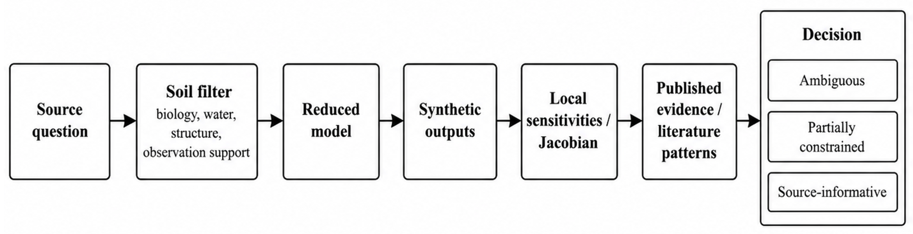
Figure 1.
Practical sequence used in the study. The source question is passed through the soil filter, including biology, water state, structure, and observation support. The reduced model generates synthetic outputs from which local sensitivities and the raw Jacobian are constructed. Nuisance-projected structural rank and the separate noise-scaled check are derived from this Jacobian and interpreted alongside published evidence and literature patterns to classify the observation set as ambiguous, partially constrained, or source-informative.
Figure 1.
Practical sequence used in the study. The source question is passed through the soil filter, including biology, water state, structure, and observation support. The reduced model generates synthetic outputs from which local sensitivities and the raw Jacobian are constructed. Nuisance-projected structural rank and the separate noise-scaled check are derived from this Jacobian and interpreted alongside published evidence and literature patterns to classify the observation set as ambiguous, partially constrained, or source-informative.
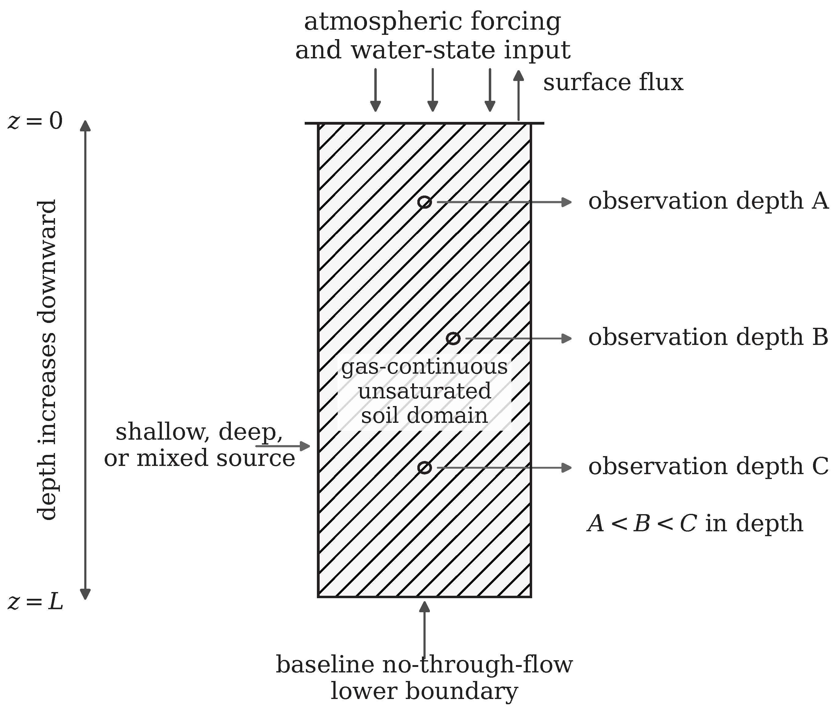
Figure 2.
Reduced one-dimensional diagnostic domain. Atmospheric forcing and the prescribed water state act at the upper boundary , while the upward arrow denotes surface emission. Integral-normalized internally distributed source supports may be shallow, deep, or mixed. Three depth-resolved observation supports satisfy . The baseline lower boundary is no-through-flow, ; no lower-boundary input is imposed in the numerical experiments.
Figure 2.
Reduced one-dimensional diagnostic domain. Atmospheric forcing and the prescribed water state act at the upper boundary , while the upward arrow denotes surface emission. Integral-normalized internally distributed source supports may be shallow, deep, or mixed. Three depth-resolved observation supports satisfy . The baseline lower boundary is no-through-flow, ; no lower-boundary input is imposed in the numerical experiments.
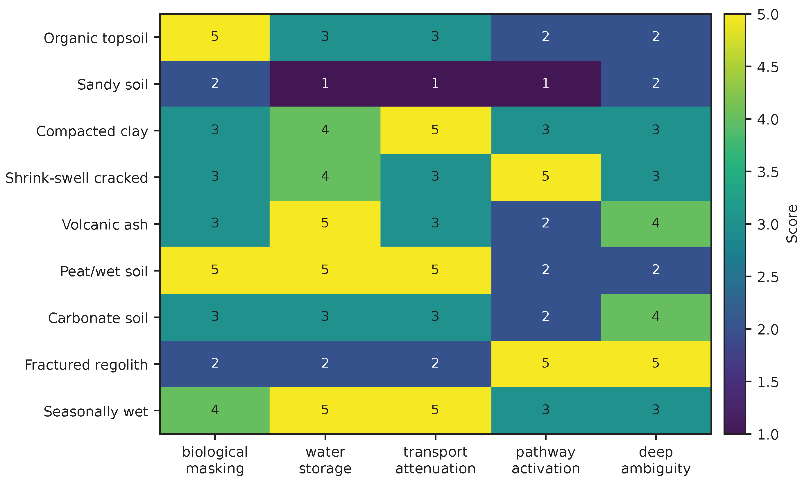
Figure 3.
Soil-type filtering scores used to connect the reduced numerical model to common soil settings. High biological masking indicates that biological carbon dioxide (CO2) production can dominate or obscure other signals. High water-state filtering indicates a strong risk of attenuation through reduced gas connectivity and, for decaying species or transient extensions, partitioning and storage. High pathway activation indicates a strong risk that structural change will be mistaken for source change.
Figure 3.
Soil-type filtering scores used to connect the reduced numerical model to common soil settings. High biological masking indicates that biological carbon dioxide (CO2) production can dominate or obscure other signals. High water-state filtering indicates a strong risk of attenuation through reduced gas connectivity and, for decaying species or transient extensions, partitioning and storage. High pathway activation indicates a strong risk that structural change will be mistaken for source change.
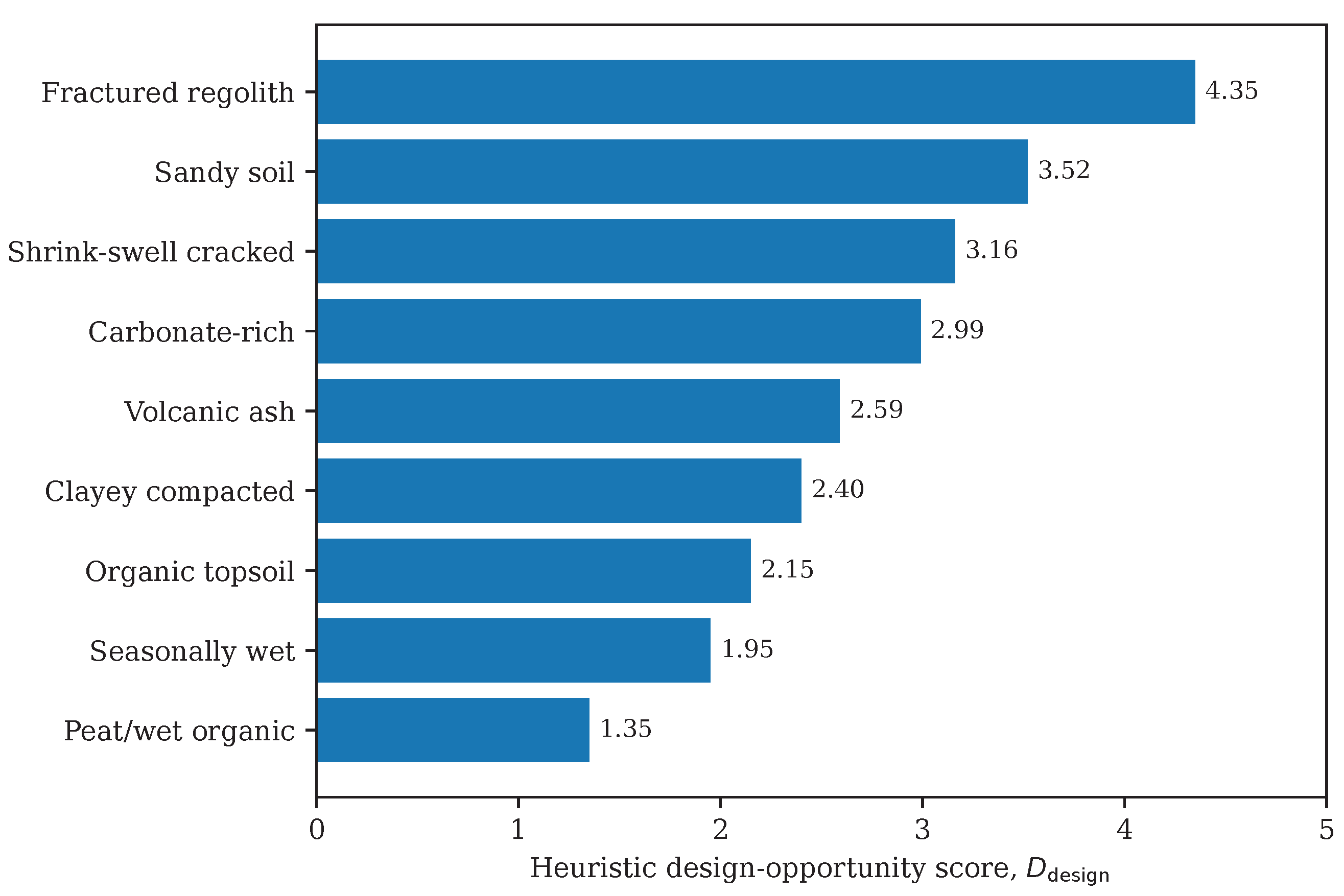
Figure 4.
Heuristic soil end-member design-opportunity score
. The formula and weights are given in the Methods, and the input scores are provided in the
Supplementary Materials. The score is an ordinal screening indicator; it is not a rank metric, a physical property, or a measure of practical source identification.
Figure 4.
Heuristic soil end-member design-opportunity score
. The formula and weights are given in the Methods, and the input scores are provided in the
Supplementary Materials. The score is an ordinal screening indicator; it is not a rank metric, a physical property, or a measure of practical source identification.
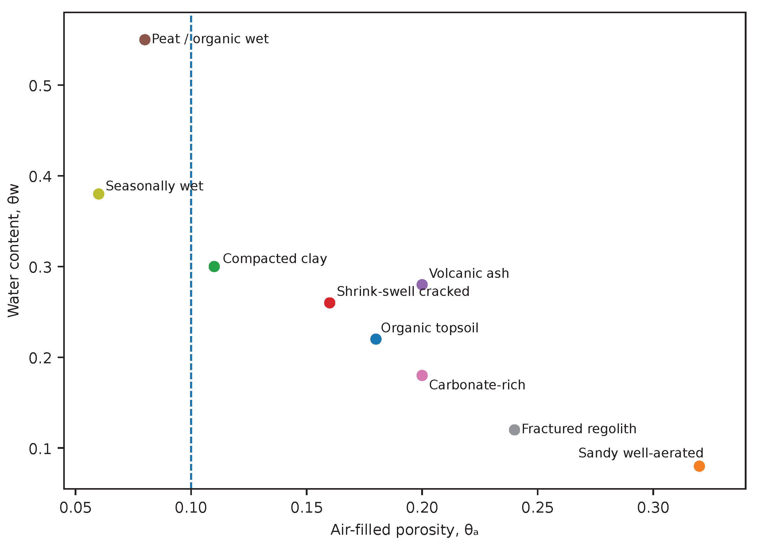
Figure 5.
Gas-continuity validity space for the synthetic soil end-members. The dashed vertical line indicates the approximate lower air-filled-porosity limit used here as a warning threshold. Points to the left are not treated as valid gas-continuous cases unless independent evidence shows connected gas pathways.
Figure 5.
Gas-continuity validity space for the synthetic soil end-members. The dashed vertical line indicates the approximate lower air-filled-porosity limit used here as a warning threshold. Points to the left are not treated as valid gas-continuous cases unless independent evidence shows connected gas pathways.
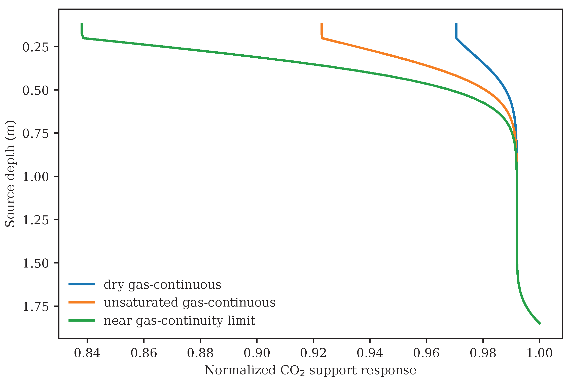
Figure 6.
Steady CO2 support response for a unit-integral source moved through the column under three prescribed water states. Lower air-filled porosity reduces effective diffusivity and changes the transmitted support response. The figure does not represent transient dissolved-gas storage or a calibrated hydraulic trajectory.
Figure 6.
Steady CO2 support response for a unit-integral source moved through the column under three prescribed water states. Lower air-filled porosity reduces effective diffusivity and changes the transmitted support response. The figure does not represent transient dissolved-gas storage or a calibrated hydraulic trajectory.
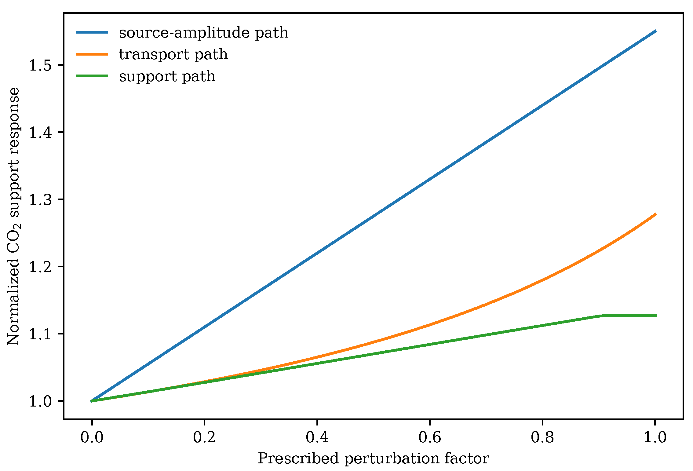
Figure 7.
Restricted-support CO2 ambiguity experiment. The horizontal axis is a prescribed perturbation coordinate, not time. Source-amplitude, transport, and support paths can generate overlapping normalized responses. The figure demonstrates attribution ambiguity, not absence of source sensitivity.
Figure 7.
Restricted-support CO2 ambiguity experiment. The horizontal axis is a prescribed perturbation coordinate, not time. Source-amplitude, transport, and support paths can generate overlapping normalized responses. The figure demonstrates attribution ambiguity, not absence of source sensitivity.
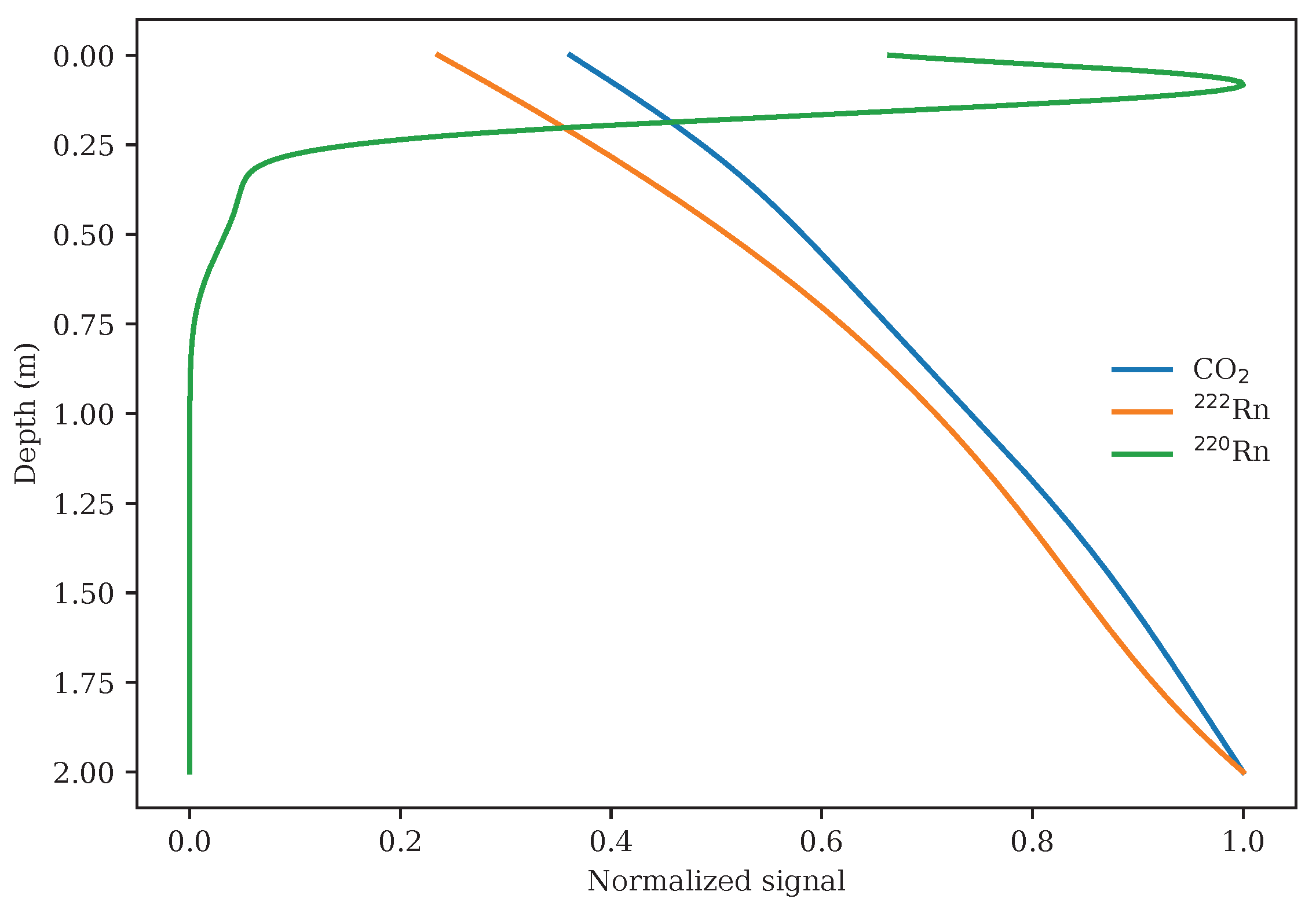
Figure 8.
Normalized steady profiles for CO2, 222, and 220. CO2 reflects the transport/source/support configuration; radon and thoron also include radioactive decay. The short thoron diffusion–decay length produces the strongest near-surface localization. Support-averaged thoron observables are the primary numerical target; pointwise near-surface profiles require finer resolution.
Figure 8.
Normalized steady profiles for CO2, 222, and 220. CO2 reflects the transport/source/support configuration; radon and thoron also include radioactive decay. The short thoron diffusion–decay length produces the strongest near-surface localization. Support-averaged thoron observables are the primary numerical target; pointwise near-surface profiles require finer resolution.
Figure 9.
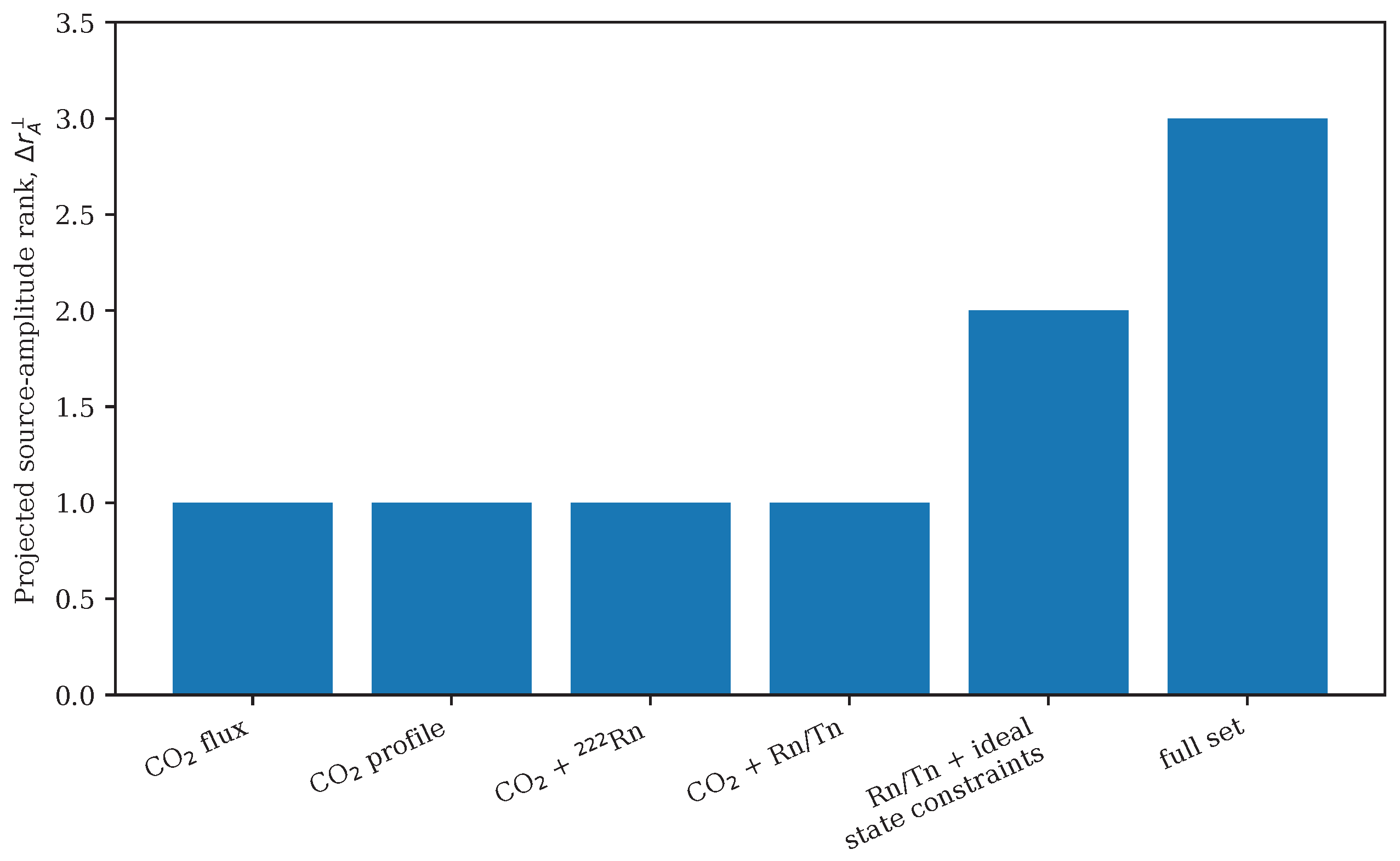
Common-threshold projected source-amplitude rank at under the primary global-before-subset column normalization. The bars count retained local source-amplitude directions after projection away from the truncated nuisance subspace. They do not count identifiable field sources and do not establish detectability.
Figure 9.
Common-threshold projected source-amplitude rank at under the primary global-before-subset column normalization. The bars count retained local source-amplitude directions after projection away from the truncated nuisance subspace. They do not count identifiable field sources and do not establish detectability.
Figure 10.
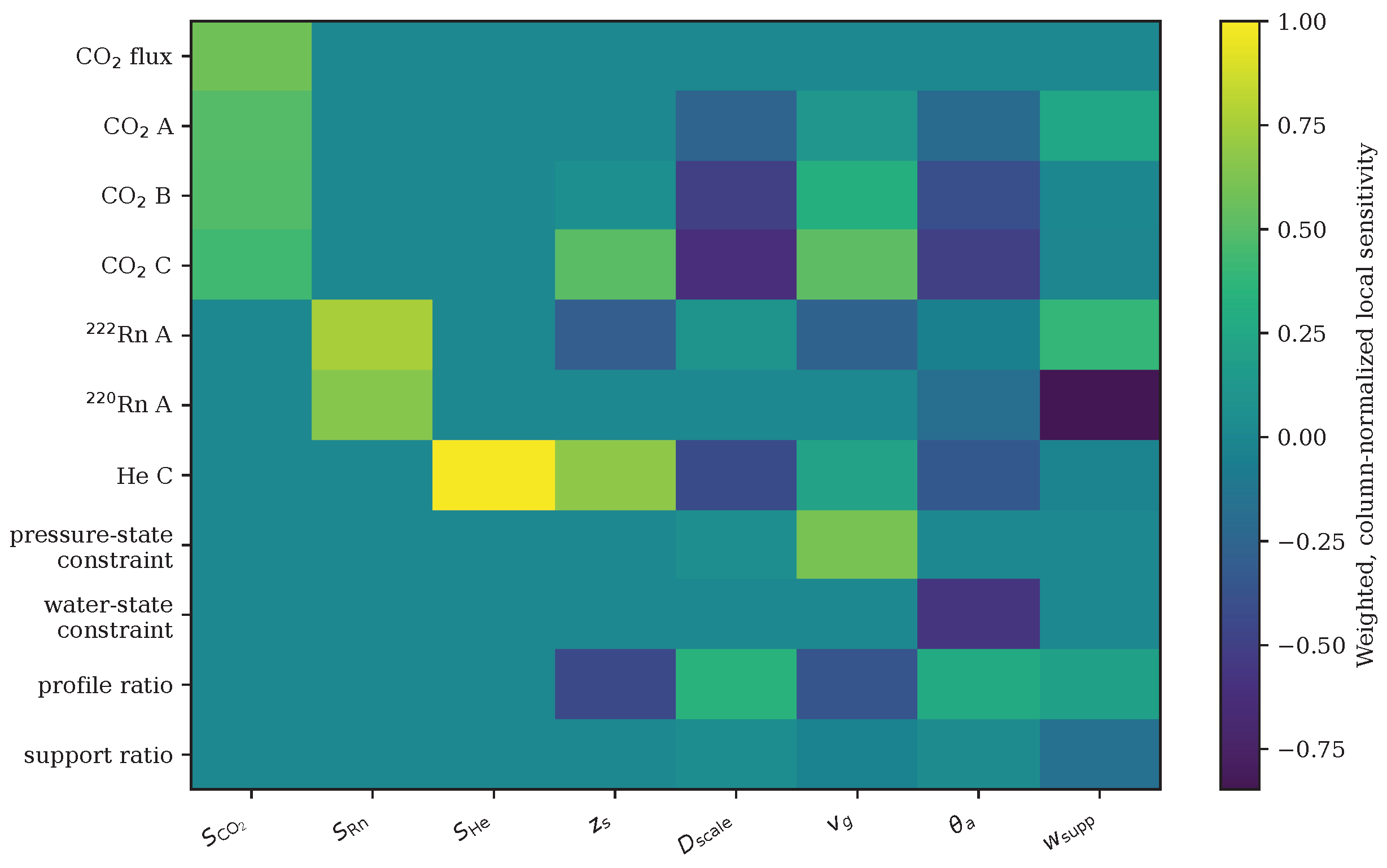
Structural sensitivity matrix for the full diagnostic set. Rows are weighted observations or idealized state constraints. Columns are , , , , , , , and . Colors show weighted, column-normalized local sensitivities used for structural screening, not raw response magnitude or a calibrated inverse solution.
Figure 10.
Structural sensitivity matrix for the full diagnostic set. Rows are weighted observations or idealized state constraints. Columns are , , , , , , , and . Colors show weighted, column-normalized local sensitivities used for structural screening, not raw response magnitude or a calibrated inverse solution.
Figure 11.
Procedure used for pattern-level consistency checking. Published studies are not used as calibration datasets. They are reduced to behavior classes, mapped to model components, assigned an evidence level, and used as targeted external consistency checks for the simulated ambiguity classes.
Figure 11.
Procedure used for pattern-level consistency checking. Published studies are not used as calibration datasets. They are reduced to behavior classes, mapped to model components, assigned an evidence level, and used as targeted external consistency checks for the simulated ambiguity classes.
Table 1.
Principal assumptions of the reduced theoretical–numerical analysis.
Table 1.
Principal assumptions of the reduced theoretical–numerical analysis.
| Assumption | Implementation | Implication |
|---|
| Geometry | one-dimensional column, m | vertical screening only; no lateral heterogeneity |
| Time treatment | steady diagnostic snapshots derived from a transient process template | no infiltration, evapotranspiration, or source-history reconstruction |
| Gas domain | gas-continuous unsaturated soil | gas-disconnected and saturated states require a multiphase model |
| Water state | prescribed , with and | hydrological state is not a Richards-equation solution |
| Spatial coefficients | , , , , and are uniform within each snapshot | depth-variable coefficients and layered flow require an extended model |
| Diffusivity closure | normalized power law | controlled closure, not a universal pedotransfer relation |
| Source representation | each Gaussian or uniform source kernel has unit depth integral before amplitude scaling | geometry changes support, not integrated source strength |
| Lower boundary | baseline with internal sources | deep scenarios are effective internal source supports |
| State constraints | pressure- and water-state rows are idealized independent nuisance constraints | they are not universal direct field measurements |
| Structural sensitivity | raw finite differences, diagnostic row weighting, then column normalization | evaluates local sensitivity geometry, not detectability |
| Noise-scaled check | raw Jacobian divided by declared observation standard deviations before any column normalization | illustrative detectability check, not a calibrated field error model |
Table 2.
Dimensional and numerical conventions used in the reduced transport equation.
Table 2.
Dimensional and numerical conventions used in the reduced transport equation.
| Quantity | Convention | Comment |
|---|
| concentration/activity per gas volume | positive model observable |
| amplitude times unit-integral depth kernel | separates source amplitude from geometry |
| spatially uniform within a snapshot | reduced air-filled-porosity closure |
| uniform reduced velocity, positive downward | negative values indicate upward motion |
| surface exchange velocity | defines |
| optional downward-positive lower-boundary flux | not used in the baseline experiments |
Table 3.
Gas-specific interpretation used in the synthetic experiments. Abbreviations: CO2, carbon dioxide; CH4, methane; He, helium; Rn, radon; Tn, thoron. CH4 is not simulated.
Table 3.
Gas-specific interpretation used in the synthetic experiments. Abbreviations: CO2, carbon dioxide; CH4, methane; He, helium; Rn, radon; Tn, thoron. CH4 is not simulated.
| Gas/Tracer | Retained Property | Interpretive Consequence |
|---|
| CO2 | mixed biological/geogenic sources; water/mineral partitioning possible | gas-phase observations may not equal total production |
| CH4 | buoyancy and oxidation sensitivity | extension relevant to landfill-cover systems |
| He | high diffusivity; atmospheric contamination | single concentration is illustrative, not a provenance proof |
| 222 | decay-limited transport over a larger support than thoron | transport-sensitive near-surface tracer |
| 220 | very short half-life | near-surface support and grid resolution are critical |
Table 4.
Main parameter groups and literature anchoring used in the synthetic experiments. Values are end-member or diagnostic choices rather than site-calibrated measurements; the full parameter table is provided in the
Supplementary Materials.
Table 4.
Main parameter groups and literature anchoring used in the synthetic experiments. Values are end-member or diagnostic choices rather than site-calibrated measurements; the full parameter table is provided in the
Supplementary Materials.
| Parameter Group | Symbol/Example | Use | Literature Basis | Limitation |
|---|
| Soil end-member labels | soil class | applicability matrix | [17,18] | not a formal site classification |
| Water and air-filled porosity | | gas-continuity and storage states | [19,20,21,22,23,24,25] | end-member ranges, not measurements |
| Gas diffusivity | | transport attenuation | [8,26,27,28,29] | reduced closure; regime-dependent |
| Gas–water partitioning | | storage/retardation | [31] | convention-dependent |
| Biological CO2 masking | , ordinal score | source ambiguity in topsoil | [32,33,34,35] | does not separate root and microbial dynamics |
| Radon/thoron behavior | , radiometric range | decay-limited sensitivity | [14,15,16,26,36,37] | not a site-calibrated radon model |
| Geogenic soil-gas ambiguity | CO2, Rn, He, source depth | deep/shallow ambiguity | [38,39,40,41,42,43,44,45,46] | pattern-level only |
| Rank diagnostics | | local separability analysis | [1,2,3] | local and tolerance-dependent |
Table 5.
Prescribed water-state cases. The phase fractions satisfy .
Table 5.
Prescribed water-state cases. The phase fractions satisfy .
| Case | | | Role |
|---|
| Dry gas-continuous | 0.32 | 0.13 | high gas connectivity with water retained |
| Unsaturated gas-continuous | 0.18 | 0.27 | baseline numerical state |
| Near gas-continuity limit | 0.10 | 0.35 | boundary-of-validity attenuation state |
Table 6.
Synthetic scenarios, hypothesis links, and evidential role.
Table 6.
Synthetic scenarios, hypothesis links, and evidential role.
| Scenario | Changed Quantity | Hypothesis | Evidence Supplied |
|---|
| CO2 ambiguity paths | , , support width | H1 | similar restricted-support responses can arise from different mechanisms |
| Water-state filtering | , with | H1/H3 | gas connectivity changes transmitted steady CO2 response |
| Radiometric profiles | decay and effective diffusivity | H2 | gas-specific depth response and short thoron length scale |
| Observation-set diagnostics | gas, profile, tracer, ideal state-constraint rows | H2 | projected source directions beyond a common-threshold nuisance subspace |
| Soil end-member translation | ordinal biological, water, attenuation, pathway, deep-source scores | H3 | heuristic, literature-anchored design implications |
Table 7.
Numerical implementation of the synthetic scenarios. Outputs are steady diagnostic snapshots rather than transient site simulations.
Table 7.
Numerical implementation of the synthetic scenarios. Outputs are steady diagnostic snapshots rather than transient site simulations.
| Scenario | Source/Boundary Treatment | Changed Quantity | Reported Output |
|---|
| CO2 ambiguity | unit-integral internal source; fixed lower boundary | source amplitude, diffusivity, support width | normalized support response paths |
| Water filtering | moving unit-integral CO2 kernel | , , source depth | normalized support response |
| Tracer profiles | fixed internal source kernels; decay retained | gas property and decay | normalized profiles |
| Structural diagnostics | linearization around baseline state | observation rows and parameter blocks | projected ranks, residuals, conditioning |
| Noise-scaled check | raw Jacobian scaled by declared observation uncertainty | same parameter blocks | singular response in one-sigma units |
Table 8.
Numerical settings used by the corrected solver.
Table 8.
Numerical settings used by the corrected solver.
| Component | Choice | Purpose |
|---|
| Domain/discretization | 2 m; 241 baseline nodes; 961-node reference | steady column and convergence test |
| Surface boundary | | upward flux observable |
| Lower boundary | | internal-source diagnostic baseline |
| Source kernels | unit-integral Gaussian/uniform mixtures | isolate amplitude from geometry |
| Structural singular-value-decomposition (SVD) floor | | suppress numerical-null nuisance directions |
| Display tolerance | , with six-value scan | transparent numerical-rank display |
| Finite differences | scaled-coordinate step | raw local Jacobian |
Table 9.
Local sensitivity coordinates. The finite-difference step is in each dimensionless coordinate.
Table 9.
Local sensitivity coordinates. The finite-difference step is in each dimensionless coordinate.
| Block | Parameters | Coordinate Scale | Mode |
|---|
| Source amplitude | | 10% log scale | multiplicative |
| Source geometry | | 0.25 m | additive |
| Transport | | 10% log scale | multiplicative |
| Gas continuity | | 0.05 volumetric fraction | additive |
| Observation support | | 0.10 m | additive |
Table 10.
Observation rows and diagnostic structural weights. The values are scale factors, not calibrated measurement-error standard deviations.
Table 10.
Observation rows and diagnostic structural weights. The values are scale factors, not calibrated measurement-error standard deviations.
| Observation Row | Weight |
|---|
| CO2 flux | 1.00 |
| CO2 A, B, C | 0.85, 0.82, 0.75 |
| 222 A; 220 A; He C | 0.80, 0.70, 0.70 |
| pressure-state constraint; water-state constraint | 0.55, 0.55 |
| profile ratio; support ratio | 0.65, 0.55 |
Table 11.
Robustness of the heuristic ranking to independent weight perturbations and renormalization over 10,000 draws.
Table 11.
Robustness of the heuristic ranking to independent weight perturbations and renormalization over 10,000 draws.
| Soil End-Member | Median Rank | Rank Range | Top-3 Prob. | Bottom-3 Prob. |
|---|
| Fractured regolith | 1 | 1–1 | 1.0000 | 0.0000 |
| Sandy soil | 2 | 2–3 | 1.0000 | 0.0000 |
| Shrink–swell cracked | 3 | 2–4 | 0.9999 | 0.0000 |
| Carbonate-rich | 4 | 3–4 | 0.0001 | 0.0000 |
| Volcanic ash | 5 | 5–5 | 0.0000 | 0.0000 |
| Clayey compacted | 6 | 6–6 | 0.0000 | 0.0000 |
| Organic topsoil | 7 | 7–8 | 0.0000 | 1.0000 |
| Seasonally wet | 8 | 7–8 | 0.0000 | 1.0000 |
| Peat/wet organic | 9 | 9–9 | 0.0000 | 1.0000 |
Table 12.
Soil-type applicability matrix for the source–transport–observation system. Scores indicate expected influence from 1, low, to 5, high. Model validity refers to the reduced gas-continuous formulation used in this study.
Table 12.
Soil-type applicability matrix for the source–transport–observation system. Scores indicate expected influence from 1, low, to 5, high. Model validity refers to the reduced gas-continuous formulation used in this study.
| Soil Setting | Bio. | Water | Atten. | Path. | Deep | Model Validity | Best Diagnostic Observations |
|---|
| Organic-rich topsoil/A horizon | 5 | 3 | 3 | 2 | 2 | Conditional | CO2 flux, C-CO2, moisture, temperature |
| Sandy well-aerated soil | 2 | 1 | 1 | 1 | 2 | Strong | CO2 profile, 222, pressure forcing |
| Clayey or compacted soil | 3 | 4 | 5 | 3 | 3 | Conditional if gas-continuous | Moisture, suction, pressure, Rn/Tn |
| Shrink–swell cracked soil | 3 | 4 | 3 | 5 | 3 | Strong with pathway term | Crack state, moisture, pressure, 220/222 |
| Volcanic ash/Andisol-like soil | 3 | 5 | 3 | 2 | 4 | Conditional; water-retention context important | CO2, Rn, water content, temperature |
| Peat/organic wet soil | 5 | 5 | 5 | 2 | 2 | Limited without hydrology | CO2/CH4, water table, redox, temperature |
| Calcareous or carbonate-rich soil | 3 | 3 | 3 | 2 | 4 | Conditional; carbonate context required | CO2, C-CO2, pH/carbonate context |
| Shallow fractured regolith/bedrock soil | 2 | 2 | 2 | 5 | 5 | Strong for mixed source–transport cases | CO2, He, Rn/Tn, pressure forcing |
| Seasonally wet or near-saturated soil | 4 | 5 | 5 | 3 | 3 | Outside reduced model when gas disconnected | Water table, redox, flux interpreted cautiously |
Table 13.
Synthetic soil end-member parameters used to translate soil class into model behavior. Values are illustrative, literature-anchored, and ordinally constrained rather than site-calibrated.
Table 13.
Synthetic soil end-member parameters used to translate soil class into model behavior. Values are illustrative, literature-anchored, and ordinally constrained rather than site-calibrated.
| Soil End-Member | | | Bio. Factor | Diff. Factor | Path. Factor | Primary Diagnostic Consequence |
|---|
| Organic-rich topsoil | 0.18 | 0.22 | high | moderate | low | CO2 masking; check temperature, moisture and isotopes |
| Sandy well-aerated soil | 0.32 | 0.08 | low | high | low | efficient gas transfer; screen with profiles and pressure |
| Clayey or compacted soil | 0.11 | 0.30 | moderate | low | moderate | verify gas continuity and hysteresis before attribution |
| Shrink–swell cracked soil | 0.16 | 0.26 | moderate | conditional | high | pathway activation may dominate anomaly |
Volcanic ash/
Andisol-like soil | 0.20 | 0.28 | moderate | conditional | low–moderate | water retention and gas connectivity control interpretation |
| Peat/organic wet soil | 0.08 | 0.55 | very high | very low | low | limited unless water-table control is measured |
| Carbonate-rich soil | 0.20 | 0.18 | moderate | moderate | low | use carbonate context; carbon isotopes |
| Fractured regolith | 0.24 | 0.12 | low–moderate | high | high | Rn/Tn/He and pressure are diagnostic |
| Seasonally wet soil | 0.06 | 0.38 | high | very low | conditional | wet gas disconnection can invalidate interpretation |
Table 14.
Pedological interpretation of the synthetic end-members. The table translates soil description into the main filter acting on source information and the practical observations needed before source attribution is attempted.
Table 14.
Pedological interpretation of the synthetic end-members. The table translates soil description into the main filter acting on source information and the practical observations needed before source attribution is attempted.
| Soil Setting | Dominant Information Filter | Main Risk If Ignored | Minimum Practical Control |
|---|
| Organic-rich topsoil | biological CO2 masking | weak non-biological signal misread | temperature, moisture, isotopes |
| Sandy well-aerated soil | fast gas connectivity | profile read as source without forcing | profile + pressure forcing |
| Clayey or compacted soil | attenuation and tortuosity | missed source or false transport change | air-filled porosity; suction/moisture |
| Shrink–swell cracked soil | pathway activation and memory | crack opening read as source pulse | pathway proxy; wet/dry state |
Volcanic ash/
Andisol-like soil | water retention and gas-connectivity filtering | attenuation read as weak source | water content; partitioning- or decay-sensitive tracers |
| Peat/organic wet soil | water table and redox control | model used outside validity range | water table, redox, temperature |
| Carbonate-rich soil | carbonate buffering and isotope exchange | CO2 assigned to wrong source | carbonate context; carbon isotopes |
| Fractured regolith | preferential pathways and lower input | pathway read as deep-source change | pressure; Rn/Tn; He or multi-gas |
| Seasonally wet soil | intermittent gas disconnection | gas anomaly read in invalid state | gas continuity and hydrological state |
Table 15.
Projected structural diagnostics at under the primary global-before-subset normalization. refers to source-amplitude directions; includes source geometry.
Table 15.
Projected structural diagnostics at under the primary global-before-subset normalization. refers to source-amplitude directions; includes source geometry.
| Observation Set | Interpretation | | | |
|---|
| CO2 surface flux | one source-related response; no attribution separation | 1 | 1 | – |
| CO2 profile | profile support adds a combined geometry direction | 1 | 2 | 6.78 |
| CO2 + 222 | one source-related direction with decay contrast | 1 | 1 | 3.03 |
| CO2 + Rn/Tn | radiometric contrast, but no extra amplitude rank alone | 1 | 1 | 4.15 |
| CO2 + Rn/Tn + ideal state constraints | two amplitude directions after nuisance-state constraints | 2 | 3 | 3.65 |
| full diagnostic set | three amplitude and four combined source directions | 3 | 4 | 4.77 |
Table 16.
Illustrative noise-scaled projected source response. The calculation uses the raw Jacobian divided by independent declared observation standard deviations before projection. Dimensions are counted at or above using a numerical tolerance of . It is not a site-specific instrument model.
Table 16.
Illustrative noise-scaled projected source response. The calculation uses the raw Jacobian divided by independent declared observation standard deviations before projection. Dimensions are counted at or above using a numerical tolerance of . It is not a site-specific instrument model.
| Observation Set | Dimensions | Largest -Scaled SV | Smallest -Scaled SV |
|---|
| CO2 surface flux | 1 | 1.000 | 1.000 |
| CO2 profile | 1 | 1.169 | 0.000 |
| CO2 + 222 | 1 | 1.059 | 0.000 |
| CO2 + Rn/Tn | 1 | 1.077 | 0.000 |
| CO2 + Rn/Tn + ideal state constraints | 1 | 1.292 | 0.000 |
| full diagnostic set | 1 | 1.472 | 0.476 |
Table 17.
Numerical robustness summary. Full outputs are provided in results/mesh_convergence.csv, results/thoron_resolution_check.csv, and results/closure_sensitivity.csv.
Table 17.
Numerical robustness summary. Full outputs are provided in results/mesh_convergence.csv, results/thoron_resolution_check.csv, and results/closure_sensitivity.csv.
| Check | Range | Outcome |
|---|
| Grid refinement | 61–961 nodes | all projected ranks unchanged |
| Baseline profile convergence | 241 versus 961 nodes | CO2 0.019%, 222 0.073%, 220 1.285% maximum normalized-profile difference |
| Thoron resolution | 0.0123 m characteristic length | support averages stable; pointwise near-surface profile needs finer resolution |
| Closure sweep | 27 closures, 6 sets, 6 tolerances | rank pattern unchanged; some high-tolerance combined ranks vary |
Table 18.
Published -data worked example based on Hodges et al. [
59] and the associated open dataset [
60]. Uncertainties are propagated from the reported regression standard errors.
Table 18.
Published -data worked example based on Hodges et al. [
59] and the associated open dataset [
60]. Uncertainties are propagated from the reported regression standard errors.
| Site | Context | Published Slope | | Diagnostic Reading |
|---|
| CFRT | non-carbonate ridgetop reference | | 0 | aerobic/diffusive reference |
| CFEMS | carbonate-bearing east midslope | | | gas deficit requires water/mineral context |
| CFWMS | carbonate-bearing west midslope | | | partial gas deficit; source-only reading unsupported |
Table 19.
Condensed targeted consistency matrix. The comparison tests whether the reduced model reproduces published behavior classes, not whether it reproduces individual sites. The complete DOI-traceable matrix is provided in the
Supplementary Materials.
Table 19.
Condensed targeted consistency matrix. The comparison tests whether the reduced model reproduces published behavior classes, not whether it reproduces individual sites. The complete DOI-traceable matrix is provided in the
Supplementary Materials.
| Literature Case | Extracted Pattern | Model Component | Comparison Type | Evidence |
|---|
| Hanson et al. [32] | root and microbial respiration can dominate soil CO2 | biological source term and topsoil masking | pattern-level | Level 1 |
| Deepagoda et al. [26] | diffusivity and air permeability depend on air-filled porosity and structure | and attenuation | semi-quantitative | Level 2 |
| Rouf et al. [11] | soil-gas transport parameters can be hysteretic | history-dependent transport state | mechanistic | Level 2 |
| Kuang, Takle and Harp [53,54,55] | pressure forcing can drive vadose-zone gas motion | reduced forcing velocity | pattern-level | Level 1–2 |
| Gil-Loaiza et al. [47] | probe design and flow affect representativeness | observation support | methodological | Level 2 |
| Nazaroff, the International Atomic Energy Agency (IAEA), and Spoto [14,15,36] | radon/thoron signals depend on production, emanation, transport, decay and closure | decay-limited radiometric module | process-level | Level 1–2 |
| Chiodini, Bini, Lombardi and Voltattorni [39,42,43] | CO2, Rn, He and isotopes reduce deep/shallow ambiguity | non-redundant tracer family | interpretive | Level 1–2 |
| Pumpanen, Kutzbach and Xu [48,49,50] | chamber and pressure conditions affect flux estimates | surface observation operator [51] | metrological | Level 2 |
Table 20.
Practical translation of the diagnostic analysis. The evidence basis is stated explicitly.
Table 20.
Practical translation of the diagnostic analysis. The evidence basis is stated explicitly.
| Ambiguity | Typical Setting | Minimum Context | Diagnostic Upgrade | Basis |
|---|
| Biological masking | organic topsoil, peat | CO2, temperature, moisture | carbon isotopes/radiocarbon when source age matters | literature and expert |
| Water-state filtering | clayey, ash, seasonally wet, compacted soils | gas profile, or moisture/suction | repeated wetting–drying and water-table context | numerical and literature |
| Transport/forcing | sandy or structured gas-continuous soil | profile, pressure, surface flux | sensitivity screen for and | numerical |
| Pathway activation | cracked clay, fractured regolith | pressure, moisture, depth-resolved gas | Rn/Tn and repeated event monitoring | literature and expert |
| Deep/shallow source class | volcanic, tectonic, carbonate settings | CO2, Rn, pressure/geology | He/Ne, He isotopes, carbon isotopes | literature and expert |
| Observation support | probe/chamber/line systems | support geometry, flow, pressure, timing | transfer and support-sensitivity correction | numerical and literature |