Article

Integrating Tacit Knowledge and AI for Digital Soil Mapping in Eastern Amazonia: Ensemble Learning, Model Performance, and Uncertainty Incorporation


by
Rômulo José Alencar Sobrinho
1,
José Odair da Silva
2,
Lívia da Silva Santos
2,
Fabrício do Carmo Farias
1,
Alessandra Noelly Reis Lima
1,
Nelson Ken Narusawa Nakakoji
1,
Daniel De Bortoli Teixeira
3,
Rose Luiza Moraes Tavares
4,
Gener Tadeu Pereira
3,
Daniel Pereira Pinheiro
5 and
João Fernandes da Silva-Júnior
1,6,*
1
Graduate Program in Agronomy (PGAGRO), Federal Rural University of the Amazon, Belém 66077-530, PA, Brazil
2
Capanema Campus, Federal Rural University of the Amazon, Capanema 68700-665, PA, Brazil
3
Department of Exact Sciences, Faculty of Agricultural and Veterinary Studies, São Paulo State University (FCAV–UNESP), Jaboticabal 14884-900, SP, Brazil
4
Graduate Program in Crop Production, Faculty of Agronomy, University of Rio Verde, Rio Verde 75901-970, GO, Brazil
5
Institute of Agricultural Sciences, Federal Rural University of the Amazon, Belém 66077-530, PA, Brazil
6
Cyberspace Institute, Federal Rural University of the Amazon, Belém 66077-530, PA, Brazil
*
Author to whom correspondence should be addressed.
Soil Syst. 2026, 10(3), 41; https://doi.org/10.3390/soilsystems10030041
Submission received: 22 December 2025 / Revised: 27 February 2026 / Accepted: 5 March 2026 / Published: 17 March 2026

Abstract

Predictive Digital Soil Mapping (PDSM) in Eastern Amazonia faces challenges due to its environmental complexity, difficult access, and scarce legacy data. While legacy soil maps contain valuable tacit knowledge, updating them requires methods that can handle uncertainty. This study evaluates the integration of old soil maps with machine learning to update soil information in Tracuateua, Pará, with a specific focus on the performance of ensemble learning and the explicit incorporation of uncertainty metrics in soil mapping units under hydromorphic influence, which, in addition to being difficult to access, are influenced by complex pedogenetic processes. We combined 270 sampling points, equivalent to the total pixels that captured the variability of soil mapping units, with environmental covariates and historical data. Several algorithms were tested, including an ensemble approach, to predict mapping units and quantify uncertainty through entropy and confusion indices. The ensemble model demonstrated improved stability and reduced classification uncertainty compared to single models, particularly in challenging hydromorphic environments. Although accuracy gains were modest, the models captured soil–environment relationships, with climate as: Annual Mean Temperature 22,000 years ago (Tmean_22k), relief: Channel Network Base Level (CNBL and altitude) and organism variables: Land Surface Temperature (LST) emerging as the main predictors. Spatialized uncertainty estimates, expressed through entropy and the confusion index, provide a practical decision-support tool for guiding field surveys and identifying areas of low mapping reliability. By explicitly transferring the pedologist’s mental model—encoded as tacit knowledge in legacy soil maps—into ensemble learning, this study presents a robust and transferable framework for updating soil maps in data-scarce tropical regions, balancing predictive performance, spatial consistency, and uncertainty-aware interpretation.

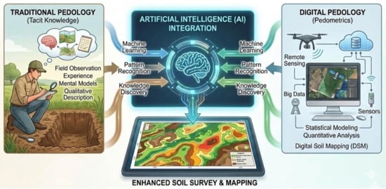
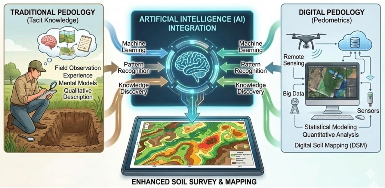
Graphical Abstract

1. Introduction

Knowledge of the spatial distribution of soils is of fundamental importance for supporting the management of environmental resources such as the atmosphere, river basins, and soil itself [1,2]. In tropical regions such as the Amazon biome, soil surveys can provide essential information for the development of projects and the planning of soil use, management, and conservation [3]. However, maps with sufficient detail to guide decision-making in the Amazon are still scarce, and the lack of high-resolution information remains one of the main limitations for sustainable agricultural planning and the implementation of conservation policies in this biome.
In Brazil, detailed soil surveys at a scale of 1:100,000 or larger cover less than 6% of the entire territory, according to information from the National Soil Program (Pronasolos). Furthermore, in the Brazilian Amazon, which covers approximately 5 million km2, the vast majority of available surveys are at a smaller, exploratory, or low-intensity reconnaissance scale (1:1,000,000 to 1:250,000). Among the challenges hindering the slow progress of soil surveys in this biome since the late 1980s, when the RADAMBRASIL project was completed, are the vast territory and poor accessibility (except via major waterways) [4], which demands time and considerable availability of human and financial resources [5].
In this context, many studies have addressed the possibility of not only increasing the level of detail in legacy maps using predictive digital soil mapping (PDSM) techniques [6], but also incorporating uncertainty into these estimates [2]. The formalization of the PDSM, based on the SCORPAN approach published by [7], is performed by adding the spatial position (n) to the soil formation factors formulated by [8]. It allows for the prediction of soil distribution patterns or attributes in the landscape based on their relationship with environmental covariates through mathematical and statistical methods, generating a spatial model [6].
Thus, PDSM consists of developing an empirical predictive model using statistical and mathematical methods, which combines, in short, environmental information and the tacit knowledge of soil scientist, the latter materialized in conventional soil survey maps [9]. This predictive model, however, is also capable of learning the implicit uncertainty of soil classes from legacy maps [10]. The uncertainty of the predictions is related, among other causes, to the quality of the database and the variability of the soil [11]. In this sense, considering pixel-by-pixel conversion from a soil mapping unit, in which the target is classified according to its similarity to the object, it can be evaluated by the degree of certainty in a pixel classification, which is associated with a specific soil class or attribute [11].
The possibility of improving mapping quality based on legacy maps has been addressed in a literature review of 90 publications related to digital land mapping and modeling [12] and in a study [13] exploring the potential of machine learning to accelerate the mapping of parental soil material in the northern region of Europe. In our work, we propose improvements in the Amazon biome. In traditional mapping, among soil formation factors, relief is the factor that strongly depends on the soil scientist’s tacit knowledge and the subjective interpretation of the morphogenetic criteria used to establish soil–landscape relationships [14,15]. Ref. [16] also highlights how protocols such as the Cornell method, along with other systematic evaluation approaches, reveal the subjectivity and variability in the quality of historical information contained in traditional soil survey maps, whose cartographic generalization results in greater spatial uncertainty [17].
When combined with field pedological knowledge and important pedogenetic predictive covariates [18], PDSM becomes a more efficient, reproducible, and economical approach to reduce soil information gaps, like in the Amazon biome, where detailed scale soil surveys are widely scarce and economically challenging in the context of the territorial dimension of the Brazilian Amazon. This approach helps to overcome the limitations associated with the subjectivity of tacit knowledge applied in traditional soil surveys [19] and has shown particular promise in addressing the challenges posed by traditional maps, whose spatial and textural accuracy often does not correspond to their nominal publication scale, thus limiting their usefulness for detailed assessments [16].
The use of machine learning-based modeling techniques—integrating field samples, pedological knowledge, and interrelated environmental variables—constitutes the conceptual core of PDSM [20]. Among the algorithms most commonly applied in pedometric studies are Random Forest, Ranger, XGBoost, and C5.0, all based on decision tree structures. These methods have become fundamental for PDSM due to their ability to model complex nonlinear relationships, handle high-dimensional predictor spaces, and capture interactions between multiple environmental covariates [21,22,23]. Furthermore, ensemble learning approaches have gained increasing prominence by combining predictions from multiple algorithms, resulting in more robust models with lower variance and superior predictive performance compared to individual learning [24,25,26].
This study addresses the improvement of a soil map published in 1998 for the municipality of Tracuateua, with a scale of 1:100,000, in northeastern Pará, by integrating PDSM, environmental covariates, and multiple machine learning algorithms, including ensemble modeling. Its innovation lies in improving the detail of soil maps for the Amazon biome, focusing on soils in hydromorphic environments, known for their high pedogenetic complexity and difficulty of access. It explicitly examines the implications of using legacy maps as training labels and the spatial dependence of the models in the context of evaluating the uncertainty of the predicted maps.
Given this, our hypothesis is that ensemble modeling increases the stability of predictions and reduces the spatial uncertainty in predicting soils under hydromorphic environments compared to individual models. Therefore, the objectives of this study were (i) to compare the predictive performance of different machine learning algorithms, (ii) to analyze the effect of ensemble modeling on the stability of predictions, and (iii) to quantify and interpret the spatial uncertainty of classification, with an emphasis on soils under critical areas for field surveys such as in hydromorphic environments.

2. Materials and Methods

2.1. Study Area

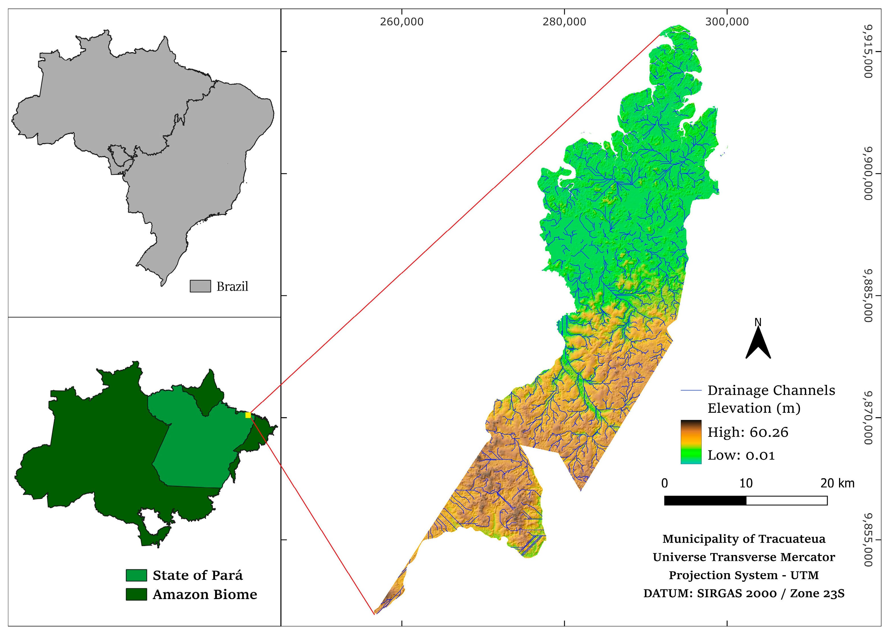
The study area encompasses the municipality of Tracuateua, covering 828.025 km2 and located within the Amazon biome in the northeastern Pará mesoregion, between approximately 01°02′ S latitude and 46°56′ W longitude (Figure 1). The regional climate is classified as Am—tropical monsoon—according to the Köppen system, with a mean annual precipitation of 2581 mm and a mean annual temperature of 27.8 °C [27]. This tropical climatic regime strongly influences soil weathering processes, acting in conjunction with the parent material and the variability of geomorphological positions that structure the local landscape [3].
The study area is characterized by the predominance of sediments from two geological periods. (i) The Quaternary period is represented by recent alluvial deposits along the banks of large rivers such as the Japerica River, as well as beaches and mangroves. In these hydromorphic environments, GLEISSOLOS HÁPLICOS, NEOSSOLOS QUARTZARÊNICOS Hidromórficos, and PLINTOSSOLOS, according to the Brazilian Soil Classification System (SiBCS), represent common soil classes in Amazonian hydromorphic landscapes (floodplains, lowlands, and transition areas); and (ii) The Tertiary period is represented by the Barreiras Formation, which occupies approximately 70% of the study area and forms a lower Amazonian plateau characterized by LATOSSOLOS and ARGISSOLOS, predominate under flat to gently undulating relief. These highly weathered soils typically exhibit yellow to red hues associated with the presence of iron oxides, which exert strong control over their spectral behavior. Soil reflectance in the visible (VIS) and near-infrared (NIR) regions is primarily governed by soil color and mineralogical composition, particularly iron oxides, clay minerals, and organic matter. The dominance of hematite and goethite in these tropical soils results in characteristic spectral patterns and reflectance variations in the VIS–NIR range. In contrast, soils formed under hydromorphic conditions—where prolonged water saturation promotes iron reduction and organic matter accumulation—generally exhibit lower reflectance and weaker spectral features, often associated with grayish or bluish colors typical of gleyed environments [28,29,30].

2.2. Data Sources

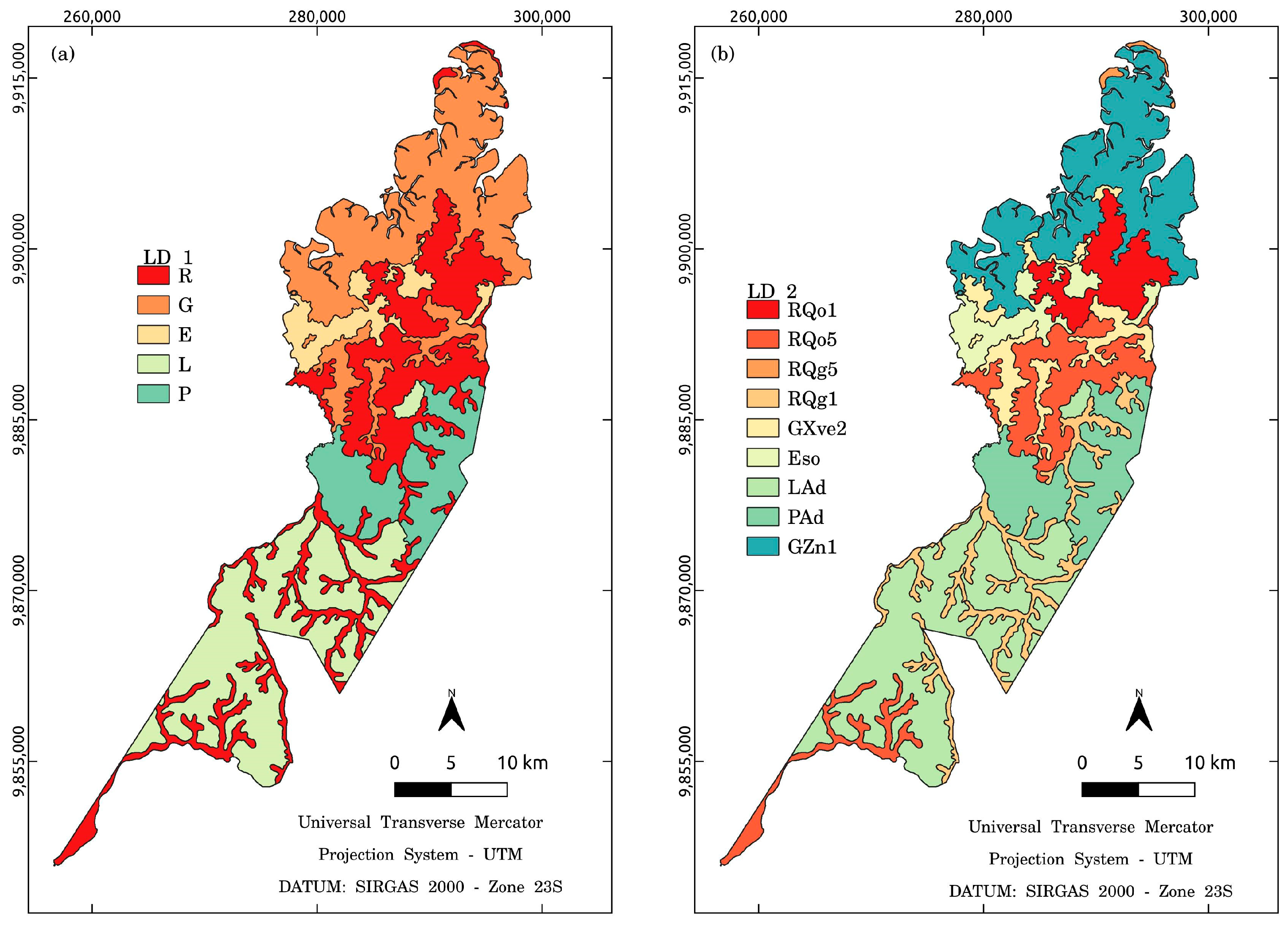
The database is composed of mapping units (MUs) defined in the conventional soil map of the municipality of Tracuateua, originally produced by [31] at a scale of 1:100,000. This legacy soil map was published at the Great Group level, according to the SiBCS, and grouped into 9 MUs (Table 1).
To enhance the predictive performance of the PDSM models, the original MUs were reorganized into two levels of detail:
(i) LD1, the least detailed level, comprising five mapping units composed of simple taxonomic units and associations at the Soil Order level derived from the legacy map; and (ii) LD2, the most detailed level, comprising nine mapping units composed of simple taxonomic units and associations at the Great Group level present in the original legacy soil map (Figure 2a,b).
This hierarchical structuring aimed to evaluate model sensitivity under different taxonomic resolutions and to explore the effects of class aggregation on classification accuracy and uncertainty.
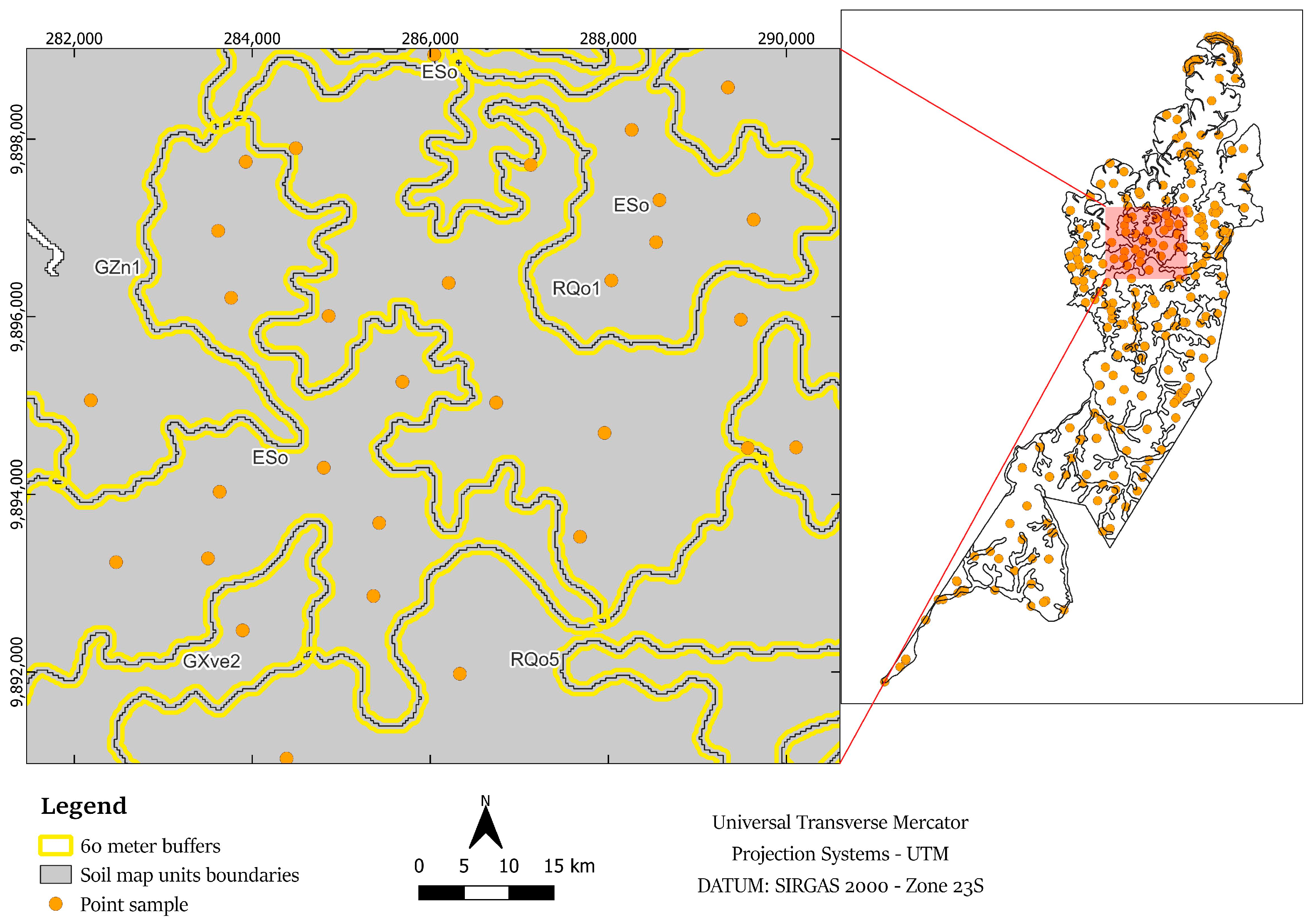
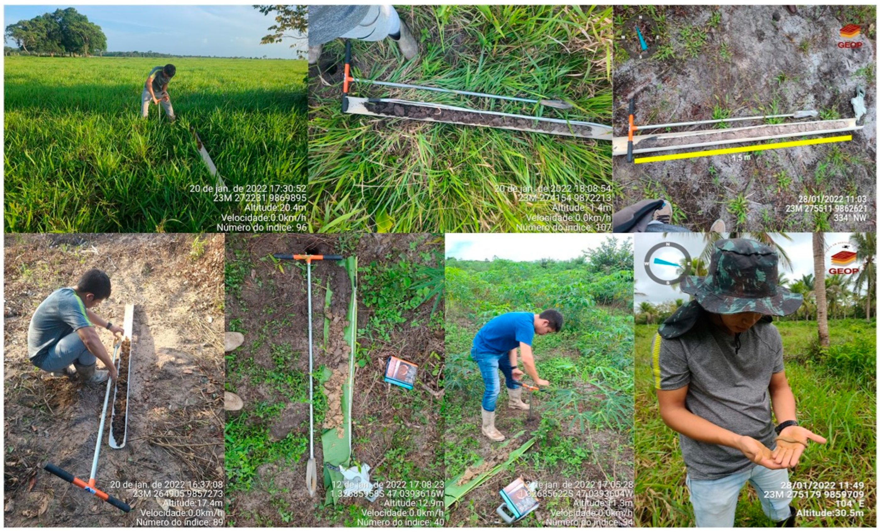
For model training, 270 pixels of 30 m × 30 m each (900 m2) were selected, aiming to guarantee the spatial variability of the pedons at both detail levels LD1 and LD2, thus covering the entire study area (828 km2). Field surveys using an auger, at a depth of 0 to 1.50 m, were carried out in the area of the aforementioned 270 samples with the objective of, in addition to confirming the MUs described in the legacy soil map (Table 2), avoiding transition zones between the MUs (Figure 3 and Figure A1 in Appendix A), thus establishing a robust protocol to guarantee the independence between the MUs training. This method sought to overcome the challenges of sparse regional inference, which is due to the logistical challenge of soil surveying in the Amazonian environment. This approach allows for the identification of areas where the uncertainty of the prediction, such as the entropy and confusion index, may require additional field investigations.

2.3. SCORPAN Covariates

Fifteen predictor covariates were pre-selected based on their pedological relevance to the MUs in the study area (Table 3), aiming to align machine learning techniques with knowledge discovery approaches [10]. These covariates represent soil-forming factors following the SCORPAN framework [7]: S—soil properties or classes; C—climate; O—organisms; R—relief; P—parent material; and A—time (age).
The climate factor was represented by annual average precipitation (AAP) and paleoclimatic variables PR_22K and Tmean_22K, derived from data estimated 22,000 years ago [6]. Climate is a key driver of soil formation, and tropical conditions promote the development of highly weathered soils. Relevant datasets and models for the study area are available from Google Earth Engine (GEE) and WorldClim at 1–6 km resolution [32,33].
Table 3. SCORPAN covariates used for predictive modeling based on pedological relevance.
SCORPAN FactorsAbbreviationDescriptionSpatial Resolution/ScaleSourceReferences
Climate (C)AAPAverage Annual Precipitation6 kmGoogle Earth Engine. ImageCollection (‘UCSB-CHG/CHIRPS/DAILY’). Time series from 1981 to 2023[34]
PR_22KAnnual Precipitation 22,000 Years Ago1 kmhttps://geodata.ucdavis.edu/climate (Accessed on 31 July 2024)
Tmean_22KAnnual Mean Temperature 22,000 Years Ago5 kmhttps://geodata.ucdavis.edu/climate/cmip5/2_5m/ (Accessed on 31 July 2024)
Organism (O)SAVISoil-Adjusted Vegetation30 mMultispectral data. LANDSAT 8—sensor OLI (U.S. Geological Survey). Equation: (NIR-RED)/(NIR + RED + L) × (1 + L)[35]
LSTGround Surface Temperature—during the day1 kmGoogle Earth Engine. ImageCollection (“MODIS/061/MOD11A1”). Time series from 2000 at 2024[36]
Relief (R)CNBLChannel Network Base30 mCopernicus GLO-30 (DSM) and ANADEM (DTM). SAGA GIS 9.3.1[37]
Level
DDDrainage Density Copernicus GLO-30 (DSM) and ANADEM (DTM)[38]
MRRTFMultiresolution Index of30 mCopernicus GLO-30 (DSM) and ANADEM (DTM). SAGA GIS 9.3.1[39]
Ridge Top Flatness
MRVBFMultiresolution Index of30 mCopernicus GLO-30 (DSM) and ANADEM (DTM). SAGA GIS 9.3.1[39]
Valley Bottom Flatness
PFCProfile Curvature30 mCopernicus GLO-30 (DSM) and ANADEM (DTM). SAGA GIS 9.3.1[40]
RSPRelative Slope Position30 mCopernicus GLO-30 (DSM) and ANADEM (DTM). SAGA GIS 9.3.1[40]
AltitudeLevel30 mCopernicus GLO-30 (DSM) and ANADEM (DTM)[40]
Parent material (P)Geology 1:250,000IBGE (2023)[40]
IORIron Oxide Ratio30 mMultispectral data. LANDSAT 8—sensor OLI (U.S. Geological Survey). Equation: (Band 4-Red/Band 2-Blue)[41]
Age (A)GEOMGeomorphons30 mCopernicus GLO-30 (DSM) and ANADEM (DTM). SAGA GIS 9.3.1[42]
For the organism factor, the Soil-Adjusted Vegetation Index (SAVI) [43] and daytime Land Surface Temperature (LST) [44] were used. These were obtained from LANDSAT-8 OLI multispectral imagery and the MODIS/061/MOD11A1 daily time series (2000–2024) via GEE [45]. In the Amazon biome, organic matter inputs and high temperatures strongly influence particle aggregation, darkening of the surface horizon, water infiltration, soil erodibility, nutrient dynamics, and forest biomass [32].
Terrain attributes were derived using two elevation models: the Digital Surface Model (DSM) and Digital Terrain Model (DTM). The DSM was obtained from the Copernicus DEM GLO-30 (1 Arc Second), which provides global coverage at 30 m spatial resolution, selected for its free availability, high quality, and proven accuracy in tropical environments [46].
The DTM was derived from the South America Digital Terrain Model (ANADEM) [47], also at 30 m resolution. The development of ANADEM involved (i) calculating the Enhanced Vegetation Index (EVI), Normalized Difference Moisture Index (NDMI), Modified Simple Ratio (MSR), and Modified Soil-Adjusted Vegetation Index (MSAVI) from multispectral imagery acquired by the LANDSAT- 8 Operational Land Imager (OLI) and Sentinel-2 MultiSpectral Instrument (MSI); (ii) incorporating vegetation height data from the Global Ecosystem Dynamics Investigation (GEDI), collection L2A; (iii) using the DSM from Copernicus GLO-30; (iv) applying the TreeBoost machine learning algorithm to estimate bias induced by vegetation; and (v) obtaining the DTM by subtracting the vegetation-induced bias from the Copernicus DSM, accounting for correction based on the vegetation fractional cover.
Terrain covariates were derived from the DSM and DTM using the Basic Terrain Analysis module in SAGA GIS v. 9.3.1 [48], resampled to the UTM SIRGAS 2000 Zone 23S projection at 30 m resolution. These include CNBL, DD, MRRTF, MRVBF, PFC, RSP, and GEOM. Linear drainage density (DD) was calculated in ArcGIS 10.5 as the ratio of total channel length to basin area [49], according to [50], who reported its significant contribution to model performance and soil map extrapolation. CNBL, DD, MRRTF, MRVBF, PFC, and RSP represent terrain surface configuration and relate to the spatial distribution of soils across landscape scales [32]. GEOM captures terrain form patterns, allowing for intuitive classification of topographic features and providing useful estimates of surface age within the SCORPAN framework [7,42].
Information regarding geology and Iron Oxide Ratio (IOR) was sourced from Brazilian Institute of Geography and Statistics (IBGE) and LANDSAT-8 multispectral imagery, respectively. Parent material influences key soil properties, including consolidation, texture, and composition. The accumulation of iron oxides and hydroxides such as hematite and goethite occur in highly weathered soils and provides an estimate of the degree of soil weathering [32].

2.4. Machine Learning Algorithms

Machine learning algorithms are capable of modeling nonlinear relationships between SCORPAN covariates, including soil classes as targets and terrain attributes, location, and temporal series as predictor variables, which can not only improve mapping accuracy but also quantify uncertainty. In this study, four tree-based algorithms were used—Random Forest (RF), Fast implementation of Random Forests (Ranger), XGBoost (Xgb), and C5.0 (C5)—as well as an ensemble learning (EL) approach combining these algorithms (Table 3). Testing different algorithms is essential for identifying the most suitable method for local conditions [1].
The RF [51] and Ranger [52] algorithms share the following fundamental principles: (i) bagging (Bootstrap Aggregating), where each decision tree is trained on a randomly selected sample with replacement from the training set; and (ii) feature bagging, in which only a subset of features is selected for each decision tree in the forest. Final predictions are made by majority vote, as in the current classification study. Differences between the algorithms include computational efficiency, with Ranger being faster, and the use of different R packages—“randomForest” and “ranger” for RF and Ranger, respectively.
These models have three hyperparameters for optimization: (i) “ntree” (1000) for RF and “num.trees” (1000) for Ranger; (ii) “nodesize” (5); and (iii) “mtry” (set to 10). Among these, “mtry” was optimized using the “caret” package, testing 10 different values according to the number of covariates, with the value yielding the best performance selected, in accordance with [1].
XGBoost (Xgb), developed by [53], is based on gradient-boosted decision trees. In this model, new trees are created to correct the errors of the previous tree, and model performance is assessed based on the difference between predicted and observed values. Xgb offers advantages such as improved predictive performance via gradient descent, enhanced model accuracy, computational efficiency, parallel and distributed computing, and the ability to handle missing values, making it well-suited for complex prediction problems. The algorithm was implemented using the “xgbTree” package, with the hyperparameter “nrounds” set to 1000, while other hyperparameters—“max_depth,” “eta,” “gamma,” “colsample_bytree,” “min_child_weight,” and “subsample”—were optimized using the “caret” package.
C5.0, proposed by [54], is based on a broad decision tree capable of handling noise and missing data. The algorithm generates classifiers that help reduce the cost of misclassification rather than simply minimizing the error rate [55]. The C5.0 model includes three hyperparameters: (i) “trials” (100), (ii) “model” (tree), and (iii) “winnow” (false). The final model was implemented using the “C50” package.
In PDSM, a single machine learning algorithm is often used to implement the model. However, ensemble learning, which has the advantage of combining the strengths of different algorithms, remains underutilized. Ensemble learning encompasses three main techniques: bagging, boosting, and stacking. In this study, the bagging technique proposed by [51] was employed, aiming to combine similar models (e.g., tree-based) to reduce variance and increase model robustness. Final predictions can be aggregated by majority vote (hard voting) or probability averaging (soft voting), with the latter approach applied in the present study [56].
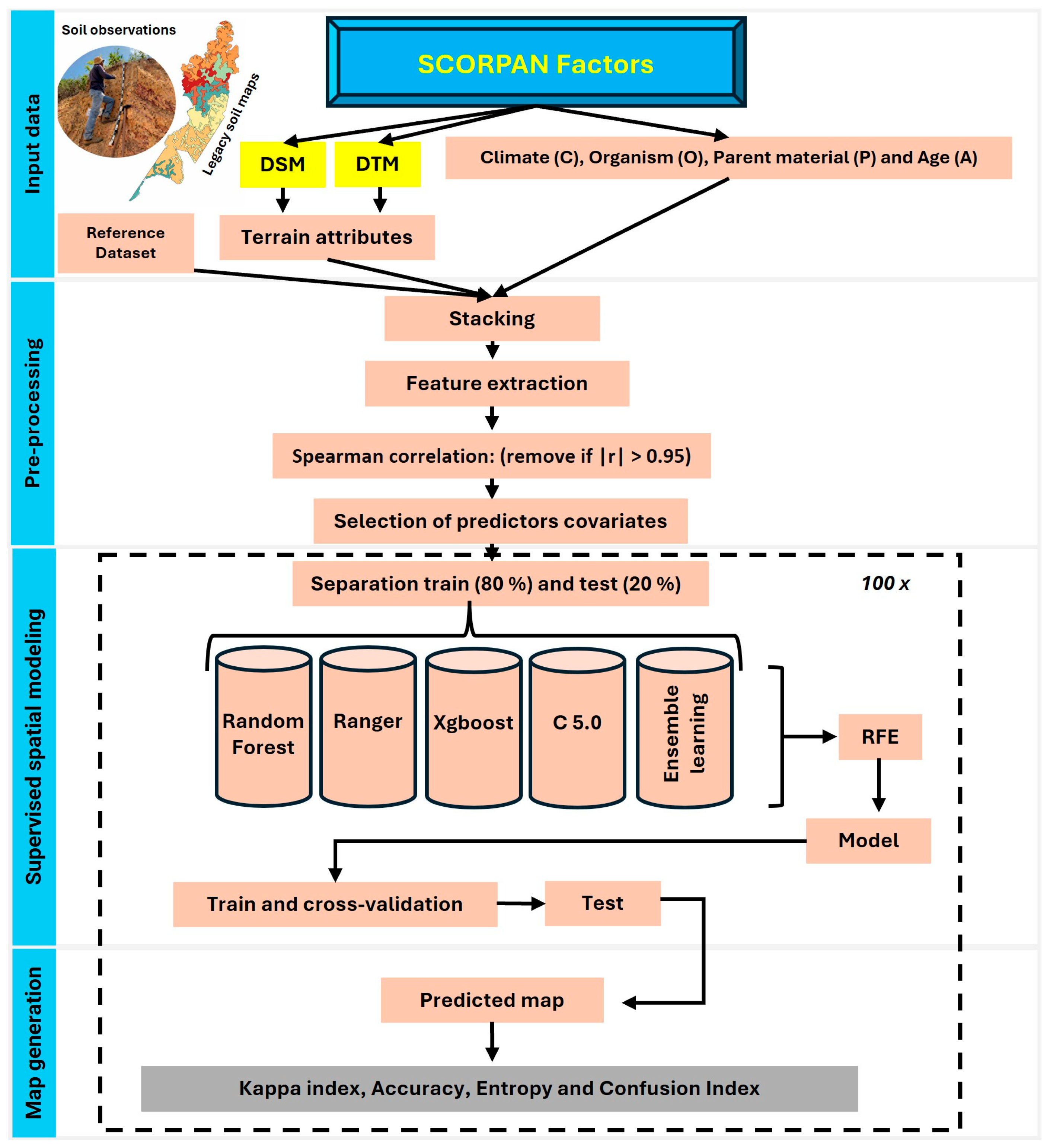
As the target, the dataset of 270 samples for both LD1 and LD2 (representing the soil taxonomic levels of Order and Great Group, respectively) was split into 80% for training with 5-fold cross-validation and 20% for testing. Using the “caret” package, this split was performed with the “createDataPartition” function, which executes more representative random sampling [1]. Subsequently, to identify the optimal subset of predictor covariates for model performance, Recursive Feature Elimination (RFE) was applied. With the adjusted parameters, 100 iterations were run, with each generated map resulting from an independent sampling iteration. The best model was selected based on the highest performance according to the Kappa index and the importance of the respective predictor covariates in predicting the targets (Figure 4).
The parameters pre-configured before the start of the process are called hyperparameters. Their selection can drastically change the model’s performance, and is essential for the reproducibility of the modeling. Therefore, in this study, we used the configurations shown in Table 4.
To represent the models used, we employed the following structure: abbreviation of the algorithm, e.g., RF, plus the origin of the terrain attributes used as environmental covariates, either DSM (S) or DTM (T), and the level of detail of the taxonomic units and associations, either LD1 or LD2. Thus, the nomenclature of the XgbS2 model, for example, means that the Xgboost algorithm was used, with terrain covariates derived from DSM, at LD2.
In this study we used Google Gemini (Free Version) to assist in refining the English translation and performing grammar checks of the manuscript text, and generating the graphical abstract figure. The results from the generative artificial intelligence (GenAI) tool were used to assist only and were carefully reviewed, edited and validated by the authors. All methodological decisions, data processing, statistical analyses, interpretation of results, and scientific conclusions were performed exclusively by the authors, who take full responsibility for the content of the manuscript.

2.5. Spatial Prediction Performance on the Test Dataset

The performance of the algorithms was evaluated using the mean Kappa index (k) and overall accuracy. The Kappa index (Equation (1)) indicates the level of agreement in predicting the mapping unit [57].
k = n i = 1 C n i i i = 1 C n i + + n + i n 2   i = 1 C n i + + n + i
where n i i is the value in row i and column i ; n i + is the sum of row i and n + i is the sum of column i in the confusion matrix; n is the total number of samples; and C is the total number of classes.
The k was interpreted using the scale proposed by [58], which defines the following ranges: Zero (0)—“Terrible,” meaning no agreement beyond chance; “Bad” (0.01–0.20); “Fair” (0.21–0.40); “Moderate” (0.41–0.60); “Very Good” (0.61–0.80); and “Excellent” (0.81–1), indicating almost perfect agreement between the models on the test data.
The Accuracy and k results from the n = 100 maps generated for each algorithm were compared using Tukey’s Honest Significant Difference (HSD) test at a 1% confidence level to assess statistically significant differences among the algorithms studied, including the ensemble learning approach (Equation (2)).
H S D = q M S E n c
where H S D is the minimum difference between two group means required for statistical significance; q is the critical value from the table; M S E is the mean squared error; and n c is the sample size for each group.
Overall accuracy, defined as the degree of agreement between model predictions and observed values, was calculated as the number of correctly classified cases divided by the total number of predictions [59], according to Equation (3).
A c c u r a c y = i = 1 C T P i N
where T P refers to the correctly classified instances of class i and C is the total number of classes, divided by the total number of cases N .

2.6. Pixel-by-Pixel Spatial Prediction Performance on the Legacy Map

The digital maps produced by the tested algorithms were compared pixel-by-pixel with the legacy soil map using the Semi-Automatic Classification Plugin (SCP) [60] implemented in QGIS Desktop 3.34.8. Model performance was evaluated through a confusion matrix, User’s accuracy (UA), Producer’s accuracy (PA), overall accuracy (OA), and Kappa index k ^ [61].
Overall accuracy (OA) measures the proportion of correctly classified pixels relative to the reference data (Equation (4)).
O A = i = 1 k n i i N
where n i i is the number of correctly classified samples for class i , corresponding to the diagonal of the confusion matrix; k is the total number of classes; and N is the total number of samples (sum of all elements in the matrix).
To properly assess UA and PA, the F1 score (Equation (5)) was calculated, which represents the harmonic mean of these two metrics. The F1 score was computed individually for each mapping unit class and ranges from 0 to 1, with values closer to 1 indicating higher predictive accuracy [62].
F 1   s c o r e = 2 U A × P A U A + P A
where U A is the percentage of samples correctly predicted for a given class relative to the total number of samples predicted for that class, also known as precision, and P A (or recall) is the proportion of samples correctly predicted for a given class.

2.7. Uncertainty of Algorithms Based on Soil Mapping Unit Classification

To estimate the prediction error of the generated digital soil maps—i.e., how close the predicted values are to the true values, also referred to as uncertainty—the probabilistic prediction of class occurrence for each mapping unit (MU) was calculated using the number of votes from the n = 100 maps generated during algorithm execution. This assessment, however, is only of practical value to the end user if it is accurate and reliable [63].
The confusion index (CI), which quantifies the uncertainty between dominant and subdominant soil classes in the mapping units (MUs) (Equation (6)) [33], and the normalized Shannon entropy [64], which measures the spatial prediction uncertainty (Equation (7)), are defined as follows:
C I = [ 1 μ m a x   i μ ( max   1 ) i ]
where μ m a x i is the probability of the most likely class for soil sampling point i , and μ ( max 1 ) i is the probability of the second most likely class for soil sampling point i . CI values range from 0 to 1, with higher values indicating greater uncertainty.
E n t r o p y = k = 1 n p k · l o g 2 ( p k ) l o g 2 ( n )
where p k is the probability of class k and n is the total number of soil classes in the mapping units (MUs). The entropy values were normalized, where 0 indicates maximum confidence in the predicted class and 1 indicates maximum uncertainty in the predictions.

3. Results

3.1. Model Performance

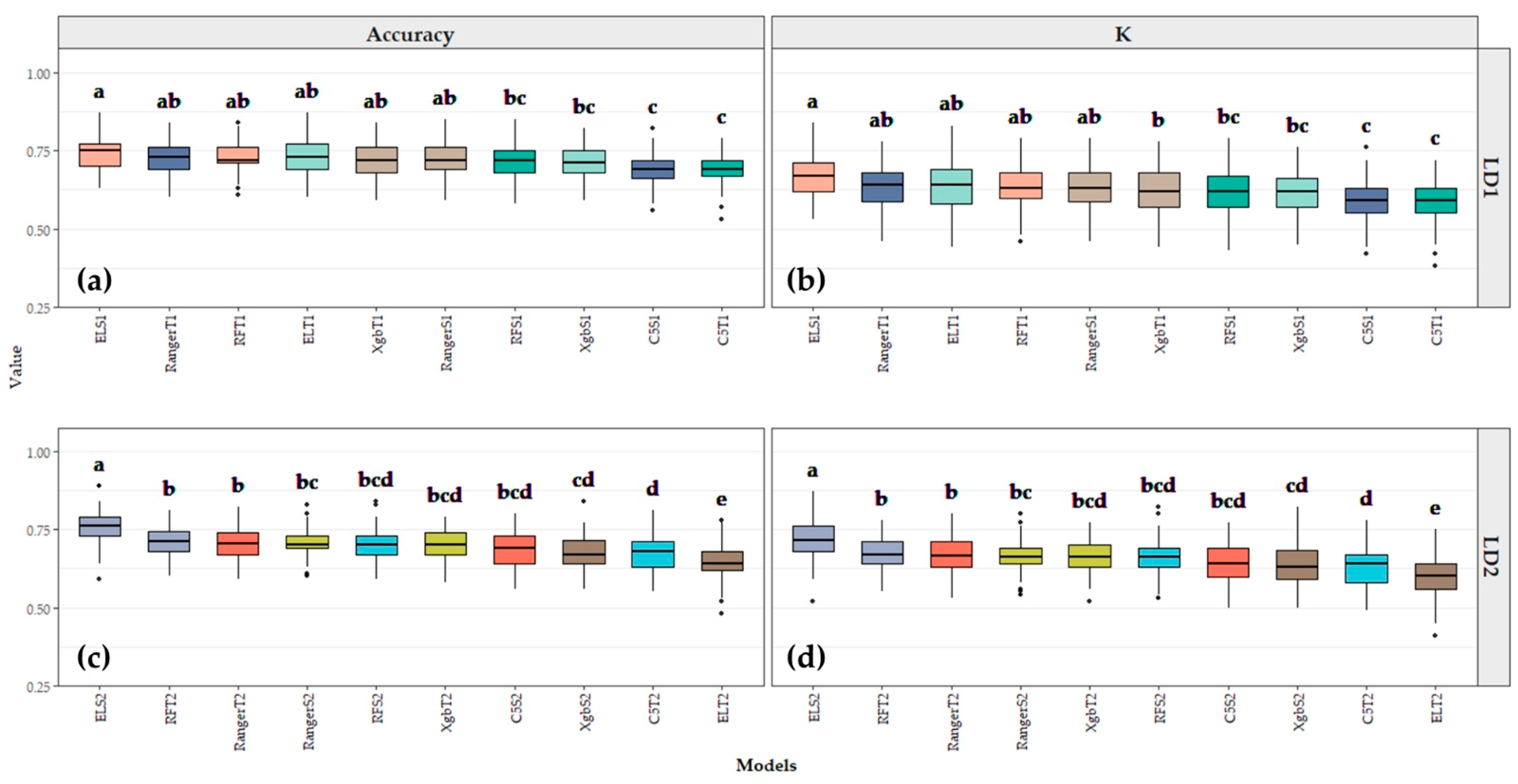
We compared the performance of the models in predicting the MUs in LD1 and LD2 (Figure 5a–d). All models presented a “very good” k (0.61–0.80), except for models C5S1 and C5T1 (LD1) and ELT2 (LD2), which obtained a “moderate” k (0.41–0.60), according to the scale proposed by [58].
In LD1, the ELS1, RangerT1, RFT1, ELT1, and RangerS1 models showed the highest average accuracy and k values, ranging from 0.74 to 0.72 and 0.67 to 0.63, respectively. In LD2, only the ELS2 model showed a higher average than the others, with 0.75 and 0.72 for accuracy and k, respectively. On the other hand, the C5 algorithms showed the lowest performance in both LD1 and LD2.
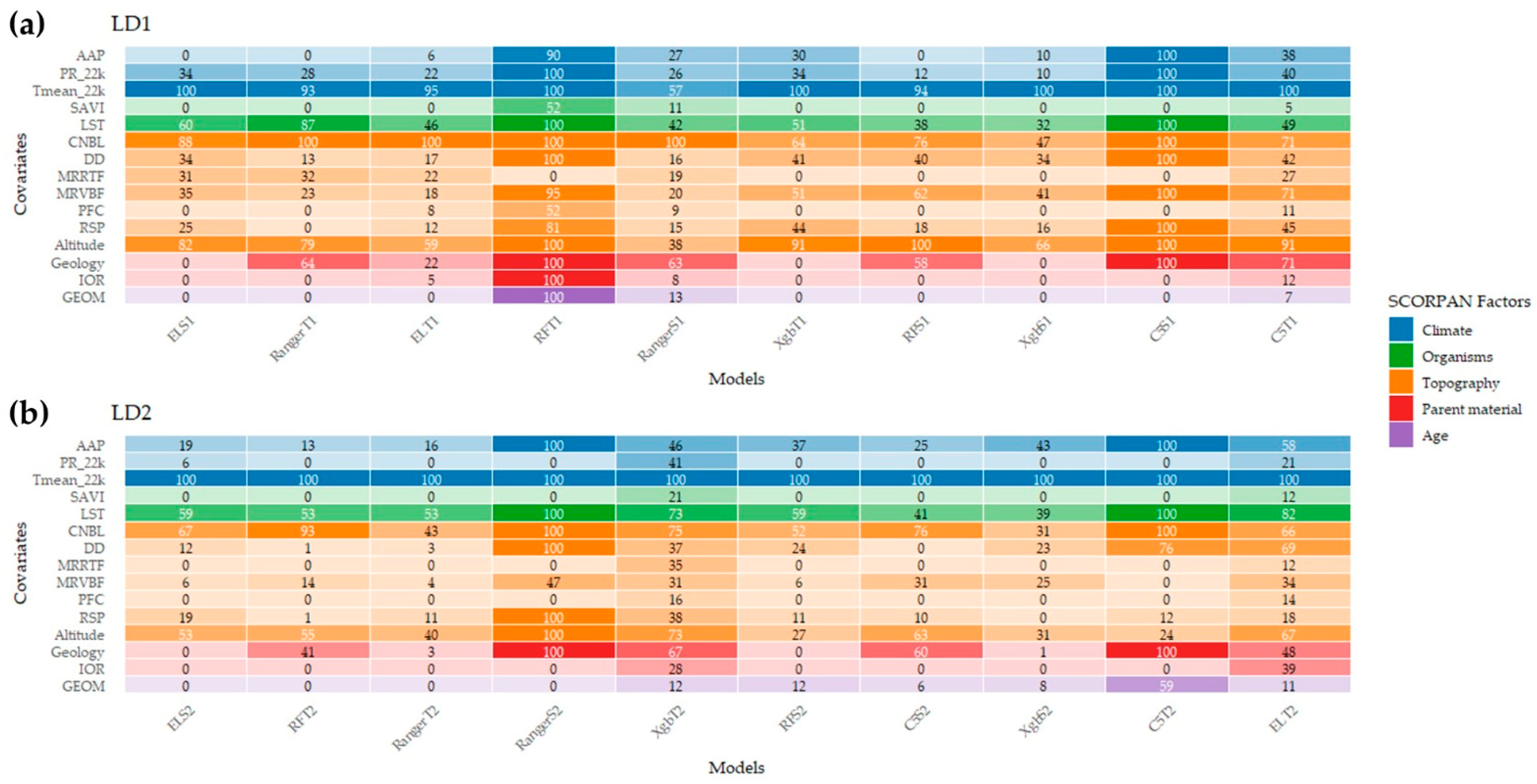
We evaluated the weight of the 15 environmental covariates in all models studied and in the prediction of soil mapping units in LD1 and LD2 (Figure 6a,b). When considering the ELS1 and ELS2 models, the environmental covariates Tmean_22k, CNBL, Altitude, and LST (ELS1) and Tmean_22k, CNBL, LST, and Altitude (ELS2) were the ones that contributed most to the models.

3.2. Internal Validation

We compared the predicted map with the legacy (reference) map, pixel-by-pixel, based on the boundaries of the predicted taxonomic units. The OA and k ^ values (Table 5) showed very little variation when comparing all of the models tested, in LD1 and LD2. Despite the reduction in the number of soil mapping units from nine in LD2 to five in LD1, we observed that the average k ^ decreased from 0.65 to 0.62.
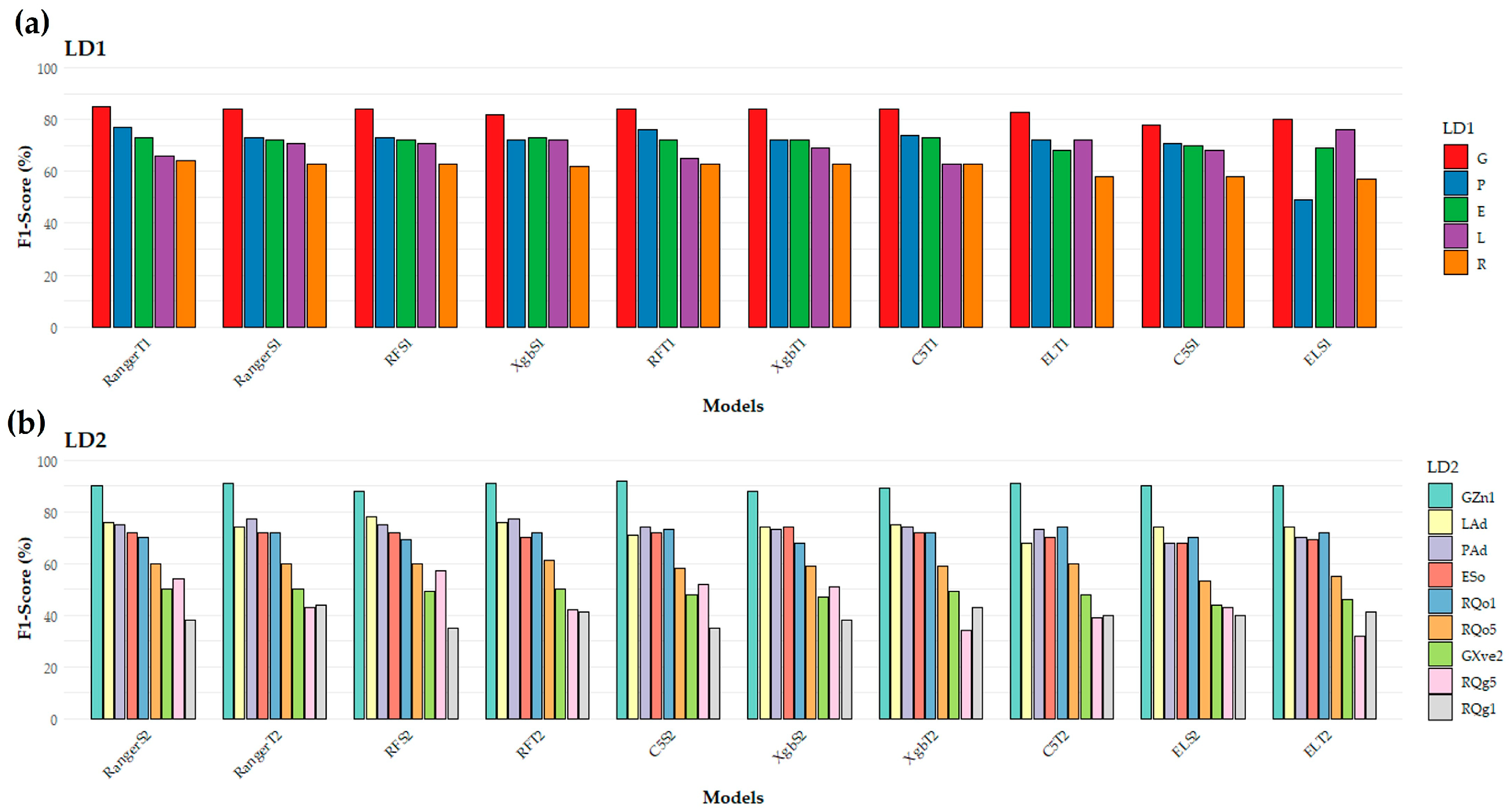
In Figure 7, we observe that the RangerT1, RangerS1, and RFS1 models in LD1 and the RangerS2, RangerT2, and RF2 models in LD2 presented the highest absolute values of PA and UA (Figure 7a,b). We observed that RQg5 and GXve2 presented the lowest PA metrics, frequently below 50% in several models, highlighting difficulties in spatial discrimination.
GZn1 showed the highest UA in almost all models—RangerS2, RangerT2, RFS2, RFT2, and C5S2—reaching 96%. The PA was also consistently high, reaching 89% in the C5S2 model. It is also worth highlighting that the high F1-score in GZn1 revealed that the climate (Tmean_22k) and topography (CNBL) factors were the most important predictive covariates in predicting this unit, which indicates soils in hydromorphic environments.

3.3. Uncertainty of Spatial Predictions

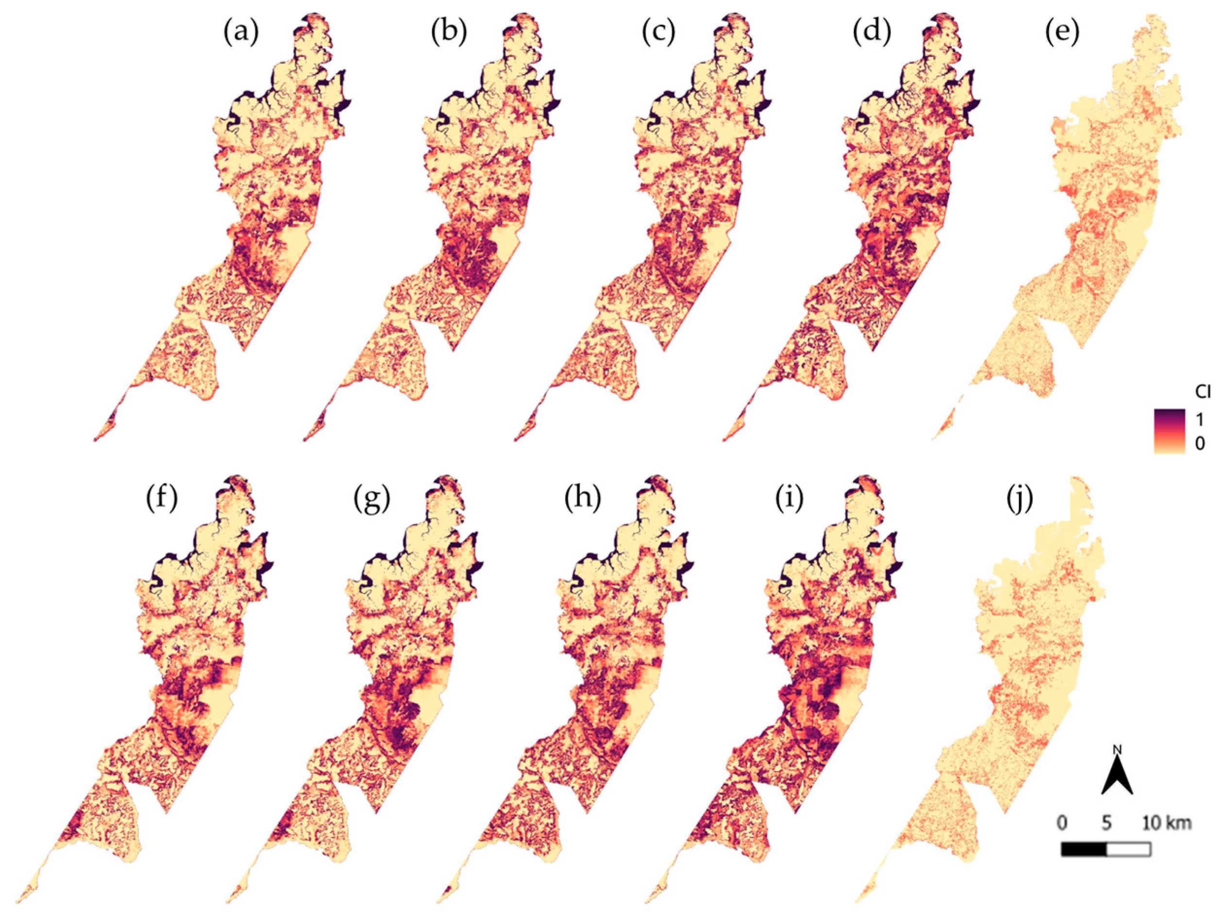
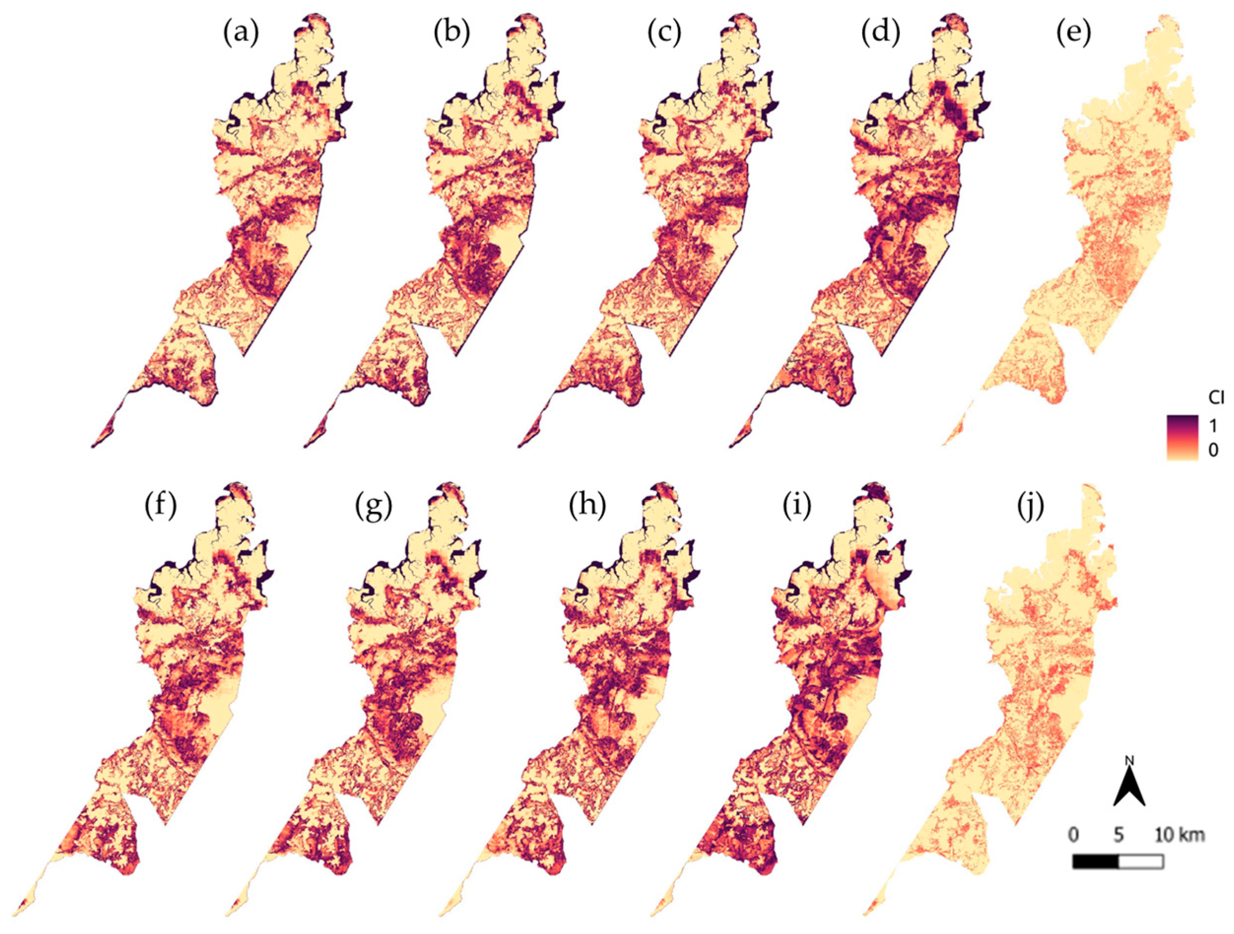
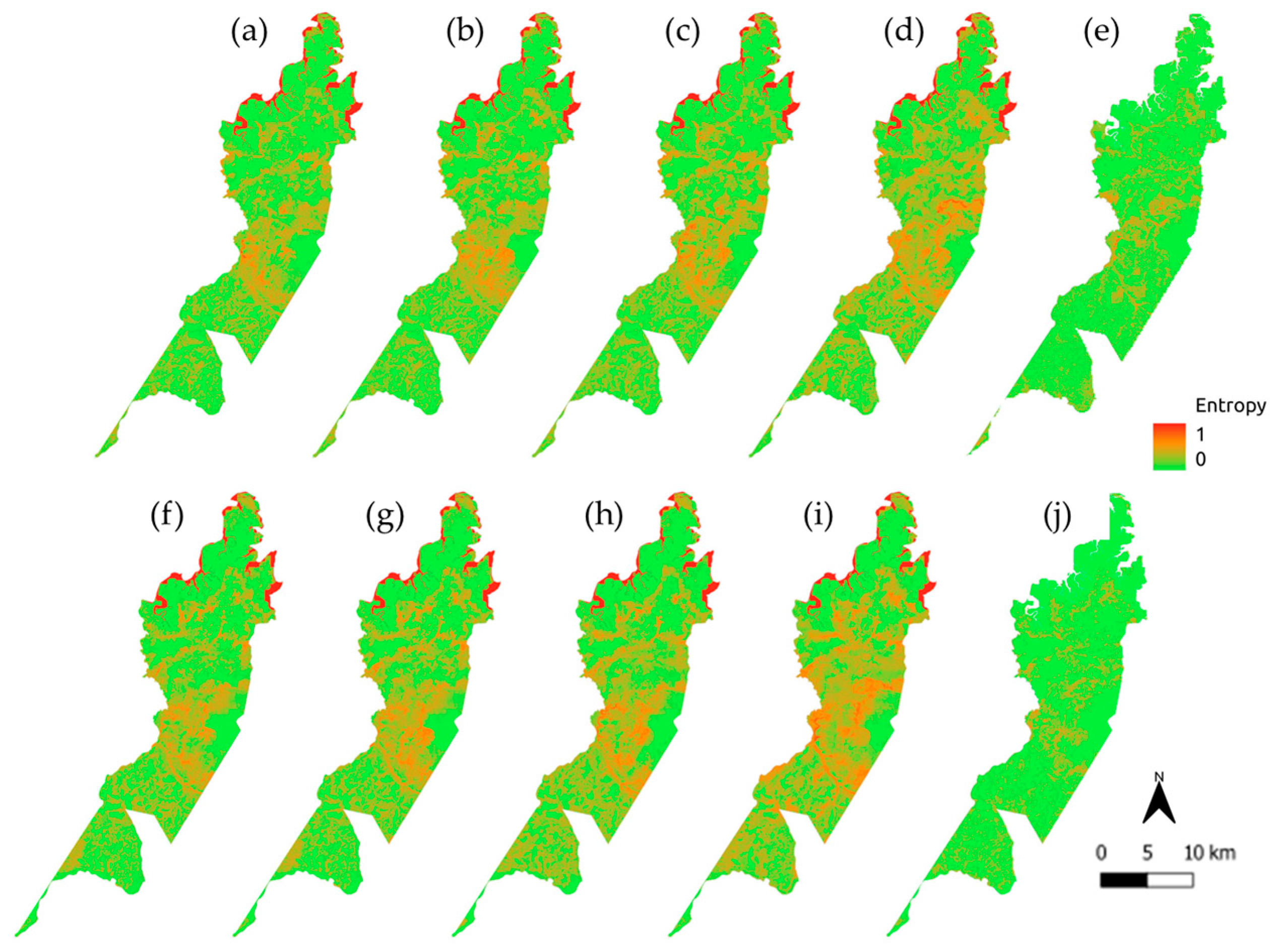
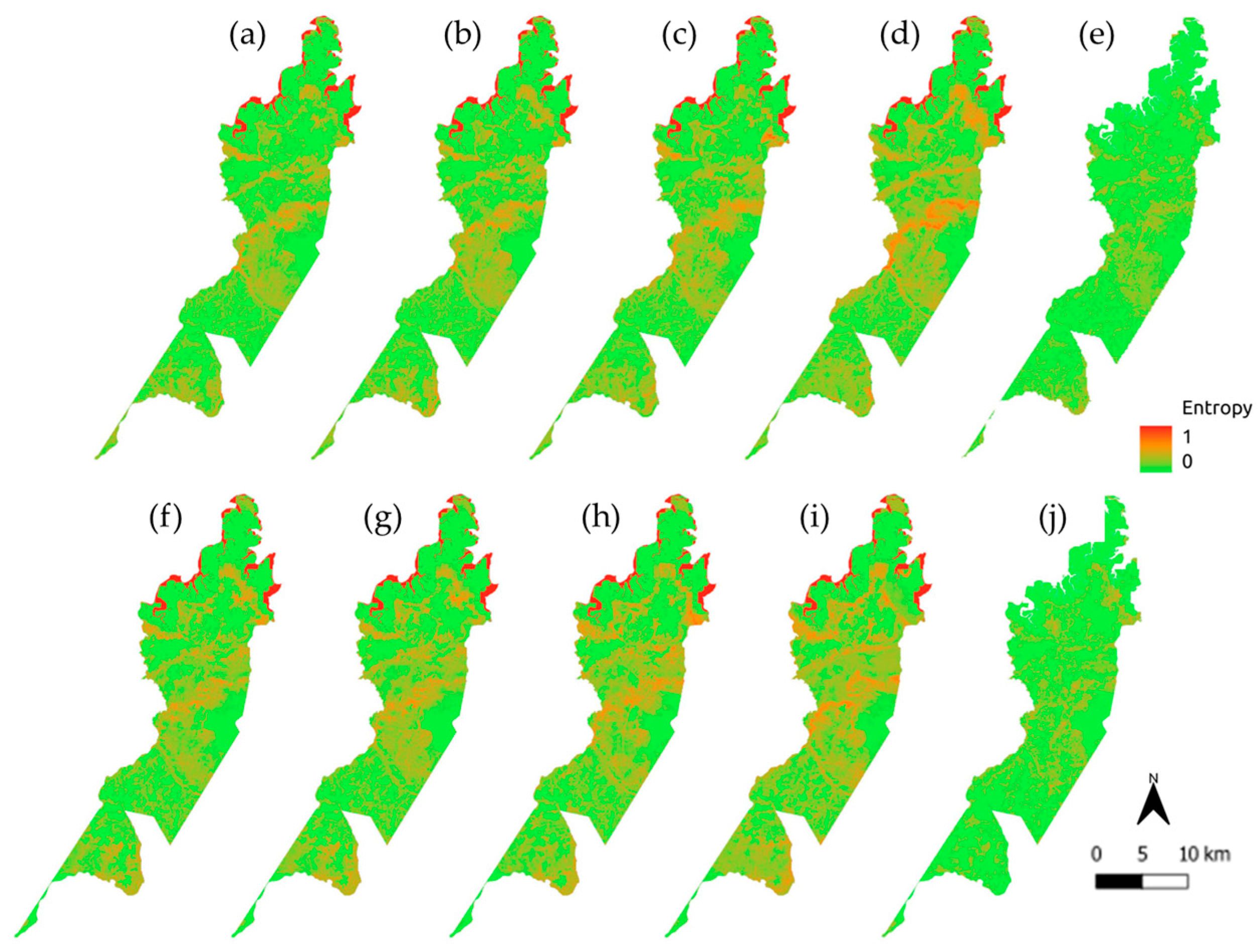
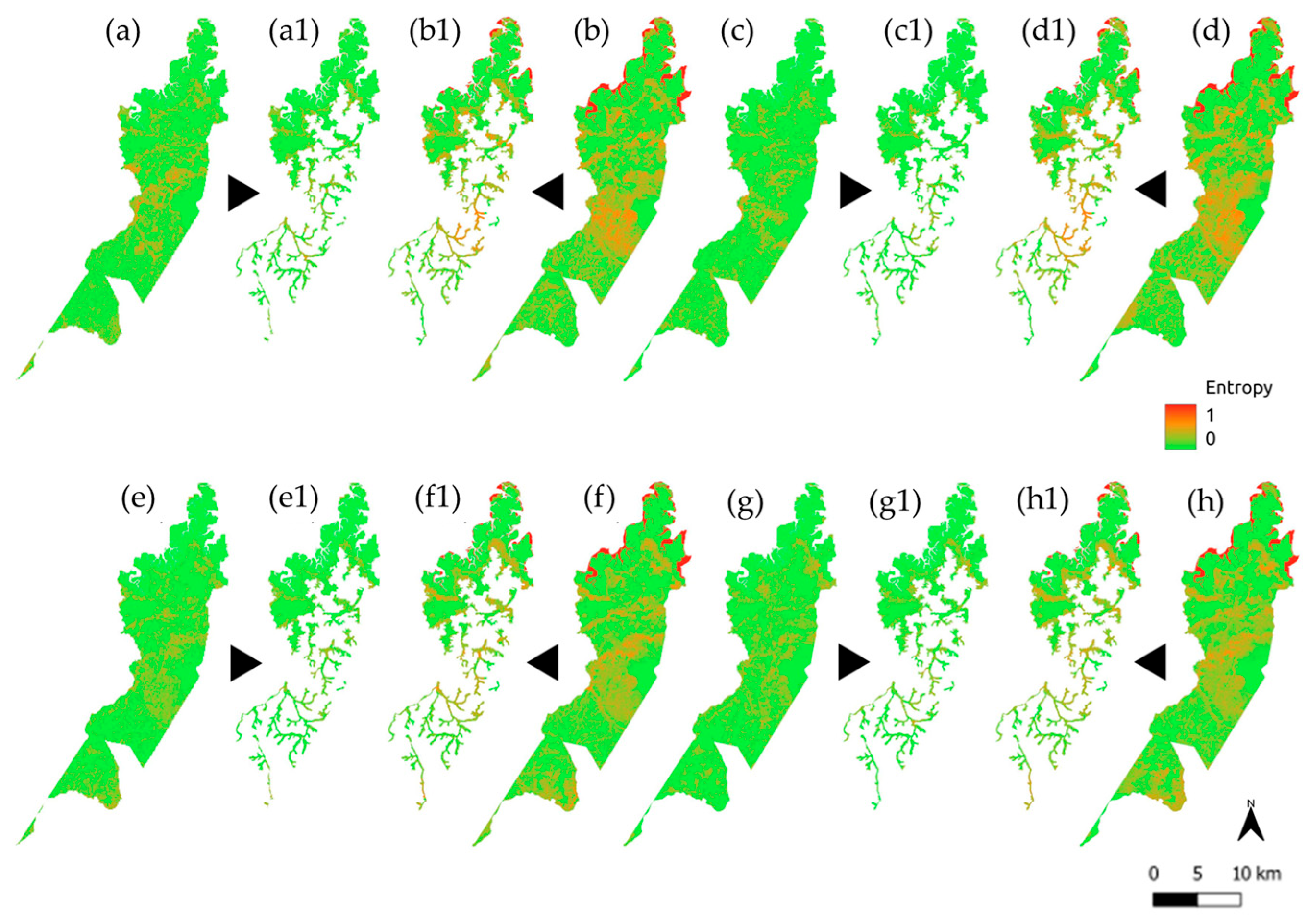
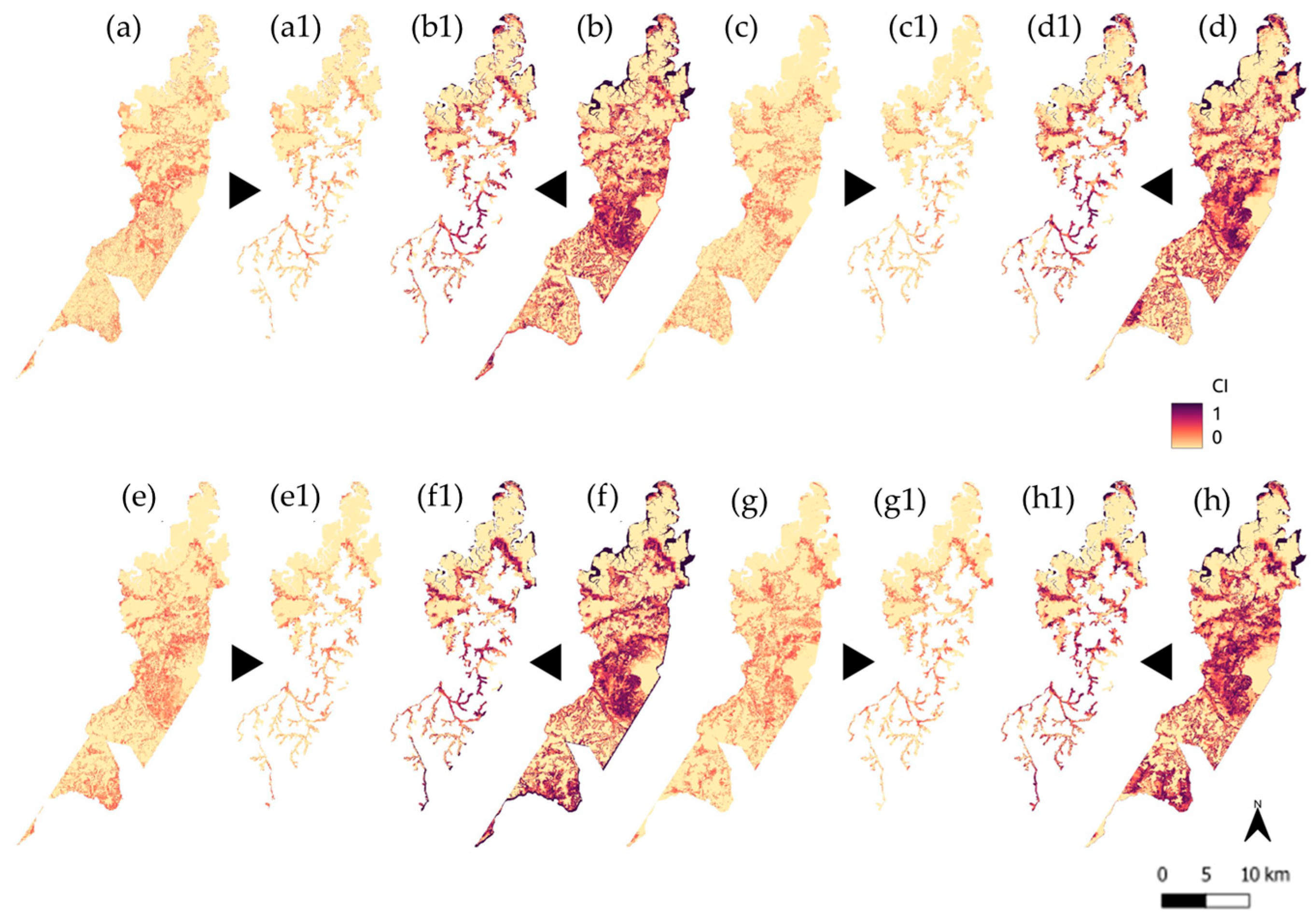
In Figure 8 and Figure 9 (entropy maps) and Figure 10 and Figure 11 (CI maps), we observe that the ELS and ELT models for both LD1 and LD2 similarly presented a larger area with predicted MUs with less uncertainty (entropy and CI close to 0) when compared to other traditional models.
The spatial uncertainty of the predictive models was further evaluated for soil mapping units under hydromorphic conditions, which are characteristic of the carbon-rich valley bottoms and alluvial plains of the Amazon. A comparative analysis of the entropy and confusion index (CI) across mapping units LD1 and LD2 is illustrated in Figure 12 and Figure 13.

4. Discussion

4.1. Evaluation of Modeling Metrics

In LD1, the stability in the prediction (Accuracy and k) of the MUs of the ELS1, RangerT1, ELT1, RFT1, and RangerS1 models was statistically higher and equal to that of the C5S1 and C5T1 models. In LD2, the stability in the prediction of the ELS2 model was statistically superior to all individual predictive models, including the ELT2 model (Figure 5).
The greater complexity of the spatial distribution of the MUs in LD2 may be related to the difference between the larger number of predictive models with higher precision and k values in LD1 compared to LD2 (Figure 5). This may be related to the potential of the EL approach to mitigate errors, mainly by using a conventional soil map as a reference. These results are consistent with those of [65,66]
Unlike our hypothesis, in general, the use of terrain attributes derived from ANADEM (DTM) and the aggregation of soil units in LD1 did not improve performance when used in modeling. This result demonstrated that the use of environmental covariates derived from DSM was sufficient in predicting soil units. The aggregation of soil units from a legacy map did not prove to be a strategy capable of improving model performance, as there was a 5-percentage point decrease in the k of ELS2 compared to ELS1 (Figure 5). This proves that despite the challenges regarding the high uncertainty implicit in the legacy map, these provide valuable information on the spatial distribution of soils [67], particularly in the Amazon region.
These results demonstrate the ability of EL to aggregate the strengths of individual algorithms. There was a 4-percentage-point difference in the k between ELS1 (0.67) and ELS2 (0.72), showing that ELS2 was more balanced than ELS1 (Figure 5), despite disagreeing with the results of [50], which justified the reduction in model performance due to the increased complexity of the MUs. In our study, the reduction in ELS1 performance compared to ELS2 may be related to error amplification by aggregating LD2 MUs to LD1 from the conventional map (reference).
The small differences in accuracy and k (Figure 5), especially in the models EL, Ranger, and RF in LD1, may be related to the fact that these algorithms all use a bagging structure, while Xgb uses a boosting structure [26,68,69].
The potential improvement in k values achieved by EL compared to traditional models for soil class prediction has been poorly reported in the literature [67]. Our results are consistent with those of [65,66], who also reported superior performance of ensemble models compared to traditional approaches. These results indicate that ELS mitigated the spatial prediction errors of individual algorithms, mainly when using a conventional soil map as a reference.
Our findings showed that paleoclimate, represented by the covariate Tmean_22k (Figure 6), was more important than the covariates representing the current climate. Similar results were found by [6], who observed the estimated precipitation from 22,000 years ago in the south of the state of Minas Gerais. During this period, it is believed that, in Brazil, a warmer and rainier climate favored erosive processes related to pedogenesis. Even in gentler relief conditions, both water infiltration into the soil profile and surface runoff can accelerate weathering [6]. Particularly in the development area of our study, characterized by its proximity to the Atlantic Ocean, this may justify the distribution of the MUs in the area.
The terrain attribute CNBL was one of the most important covariates in the ELS1 and ELS2 models (Figure 6); as a covariate derived from the drainage network, it is frequently associated with soil erosion and sedimentation and plays a key role in soil–landscape stratification [50,69,70]. The CNBL calculates the vertical distance of drainage channels, capable of separating soils under hydromorphic influence from soils in plateau areas [71]. In our work, approximately 40% of the mulches are under hydromorphic influence, which justifies this covariate being among the most important. Based on these results, we observed that the selection of uncorrelated covariates that encompass all SCORPAN factors may be related to the higher Kappa indices and precision.
These findings support the potential integration of tacit knowledge with machine learning. However, this should be approached with caution, since pedological knowledge, in addition to being reflected in the selection of relevant covariates, requires subsequent interpretation and analysis of the resulting patterns, both from a spatial prediction and soil science perspective [10,72].
We compared all models pixel by pixel with the conventional map (Table 4) in terms of the relationship between the reference and predicted MUs and by means of a confusion matrix (Table A1, Table A2, Table A3, Table A4, Table A5, Table A6, Table A7, Table A8, Table A9, Table A10, Table A11, Table A12, Table A13, Table A14 and Table A15 and Figure 7). The average value of OA in LD1 and LD2 was 0.71 and 0.70, respectively; however, the average k ^ value was 0.62 in LD1 and 0.65 in LD2. These results lead us to not indicate the aggregation of MUs. In the analysis of the F1 score (Figure 7), we observed that the individual Ranger and RF models, as well as all other models trained, in general, as MUs G in LD1 and GZn1 in LD2, obtained the highest values, indicating that all models were able to predict them.
Regarding Table 1 and Table 2, we calculated the sampling density, from which we observed that the Ranger achieved the highest F1 scores for G and GZn1, even though their densities of 0.27 and 0.18 points/km2, respectively, were the second lowest among the classes studied, represented by LD1 and LD2. In our work, the Ranger model was able to capture soil variability even with low sampling density, corroborating the findings of [22], who compared the potential of decision tree and vector learning quantization models for soil class prediction, finding greater accuracy for decision tree models in areas with low altitude variation.

4.2. Uncertainty and Practical Applications

The quantified uncertainty in PDSM is one of the main advantages over traditional soil surveys, in which the spatial distribution of mapping units or soil classes is a source of error. This reflects classification uncertainty and may be related, for example, to combined mapping units whose evaluation criteria are subjective, or to estimation models composed of coexisting soils or other generalized combinations of dominant soils [2,73].
In the study area, mapping units of hydromorphic soil classes cover more than 40% of the municipality of Tracuateua and present specific challenges, such as limited accessibility for the soil survey team. Incorporating uncertainty into the existing map can substantially assist future field surveys, reducing the time and resources required between planning and map production.
Locations with a higher entropy and confusion index, both close to 1 (Figure 12 and Figure 13), are associated with greater difficulty in pedogenesis modeling, requiring a larger number of samples to improve the quality of the soil map [67]. This demonstrates, in the present study, that models related to EL can improve the prediction of soil mapping units in areas where individual algorithms presented greater uncertainty.
Commonly represented by means of maps, the incorporation of uncertainty continues to be a major challenge in pedometrics [18,74]. In the joint analysis of the F1 score (Figure 7) and Figure 12 and Figure 13, in which uncertainty (entropy and IC) was compared, lower uncertainty values for MUs under hydromorphic conditions—G, E, RQg5, Eso, GXve2, RQg1, and GZn1—were obtained using models with the EL approach compared to Ranger. These results indicate that the overall accuracy of the map should be evaluated in conjunction with the uncertainty [63].
Valley bottom areas and alluvial plains, as shown in Figure 12 and Figure 13, are extremely common and vital geomorphic environments in the Amazon, concentrating significant carbon stocks in soils [75]. However, we believe that pedogenesis in these environments is intrinsically complex, being controlled by multiple interactive processes. According to [76], this complexity often reflects polygenesis, in which soils evolve through successive or overlapping pedogenetic processes that occur at different times or under different environmental conditions within the same landscape. This intrinsic complexity, combined with the lack of detailed soil maps for decision-making, represents significant challenges for PDSM in the region, since hydromorphic mapping units have subtle boundaries and high spatial variability, requiring high-resolution terrain covariates. Ref. [77] found that soils in hydromorphic lowlands (GXbd) were classified more accurately by some machine learning algorithms, highlighting the need for fine-scale terrain covariates. Therefore, the need to use high-resolution terrain covariates to map hydromorphic pedological units is supported by the recent review in [78].
In comparing MUs under hydromorphic conditions using the EL and Ranger models (Figure 12 and Figure 13), despite the low sample density for G and GZn1 (0.27 and 0.18 points/km2, respectively) compared to the other classes, lower entropy and CI values were observed for the EL approach. This indicates that the joint learning approach incorporated higher predictive quality in hydromorphic environments, i.e., lower uncertainty even with a reduced number of samples, corroborating the findings of [6] in their assessment of uncertainty in digital mapping of soil classes in the southern region of the state of Minas Gerais.
Given the challenges in the Amazon biome—such as budget constraints and difficult field access, particularly in hydromorphic areas—this study has shown promise for PDSM in the region [10]. Another promising application of PDSM is predictive extrapolation, which could significantly support ongoing soil surveys with higher resolution, thus helping to fill existing gaps in soil maps throughout the Amazon [79,80,81].

5. Conclusions

Considering the polygenetic nature of tropical soils, the most important covariates (Tmean_22k, CNBL, LST, and altitude) proved adequate for modeling MUs in northeastern Pará.
Despite the scarcity of validation points for some MUs in the legacy soil map of Tracuateua, the performance metrics indicate that the EL approach provided greater predictive stability than individual machine learning models, particularly in LD2 when dealing with MUs imbalance.
The results support the hypothesis that EL can discriminate MUs under hydromorphic conditions. In addition, spatial estimates of prediction uncertainty based on entropy and CI provide useful tools for guiding field surveys and improving soil classification in difficult-to-access hydromorphic areas.
Furthermore, reducing the level of detail of MUs in older maps to simplify modeling did not improve predictive performance and may increase the implicit uncertainty associated with conventional soil maps. Furthermore, despite the slightly higher use of terrain attributes derived from DSM in terms of learning model performance compared to DTM, the greater uncertainty (Entropy and CI) observed in the latter digital model may be related to the more accurate representation of terrain elevation.
However, our approach provides a framework for identifying the most appropriate use of legacy soil class data under regional constraints. The results highlight that mapping units, which are directly associated with natural landscape patterns, may be more effectively predicted by machine learning models than taxonomic soil classes, which represent conceptual groupings defined by classification systems. Consequently, mapping units tend to exhibit spatial patterns that are more readily captured by the environmental covariates used in digital soil mapping models.

Author Contributions

Conceptualization, R.J.A.S. and J.F.d.S.-J.; methodology, R.J.A.S., J.F.d.S.-J. and G.T.P.; software, R.J.A.S. and J.F.d.S.-J.; validation, R.J.A.S., J.O.d.S., F.d.C.F., L.d.S.S., J.F.d.S.-J., A.N.R.L. and D.P.P.; formal analysis, R.J.A.S., G.T.P., R.L.M.T. and J.F.d.S.-J.; investigation, R.J.A.S. and J.F.d.S.-J.; resources, R.J.A.S., J.O.d.S. and F.d.C.F.; data curation, R.J.A.S. and J.F.d.S.-J.; writing—original draft preparation, R.J.A.S.; writing—review and editing, R.J.A.S., J.O.d.S., F.d.C.F., L.d.S.S., J.F.d.S.-J., N.K.N.N., D.D.B.T., R.L.M.T. and D.P.P.; visualization, R.J.A.S. and J.F.d.S.-J.; supervision, J.F.d.S.-J.; project administration, J.F.d.S.-J.; funding acquisition, J.F.d.S.-J. All authors have read and agreed to the published version of the manuscript.

Funding

This work was supported by the National Council for Scientific and Technological Development (UNIVERSAL; public call CNPq/MCTI/FNDCT-18/2021 [Project grant no. 406838/2021-6]). This study was funded by a scientific initiation scholarship granted to the third author. Additionally, this study was financed in part by the Brazilian Ministry of Science, Technology and Innovation (MCTI) and the National Fund for Scientific and Technological Development (FNDCT).

Data Availability Statement

The original contributions presented in this study are included in the article. Further inquiries can be directed to the Corresponding Author.

Acknowledgments

We thank the members of Geotechnologies and Pedometrics Research Group—GEOP (https://geopufra.com) for their support. (Accessed on 10 March 2026). During the preparation of this study, the author(s) used Google Gemini, Free version for the purposes of refining the English translation and grammar check, and to create the graphical abstract figure. The authors have reviewed and edited the output and take full responsibility for the content of this publication.

Conflicts of Interest

The authors declare no conflicts of interest.

Abbreviations

The following abbreviations are used in this manuscript:
MUMapping Unit
LDLevel of Detail
RFRandom Forest algorithm
XgbXgboost algorithm
C5C 5.0 algorithm
ELEnsemble Learning
DSMDigital Surface Model
DTMDigital Terrain Model
AAPAverage Annual Precipitation
PR_22kAnnual Precipitation 22,000 years ago
Tmean_22kAnnual Mean Temperature 22,000 years ago
SAVISoil-Adjusted Vegetation Index
LSTLand Surface Temperature
CNBLChannel Network Base Level
DDDrainage Density
PDSMPredictive Digital Soil Mapping
MRRTFMultiresolution Index of Ridge Top Flatness
MRVBFMultiresolution Index of Valley Bottom Flatness
PFCProfile Curvature
RSPRelative Slope Position
AltitudeAltitude
GeologyGeology
IORIron Oxide Ratio
GEOMGeomorphons
RFS1RF algorithm using data derived from DSM, in LD1 of the MU
RangerS1Ranger algorithm using data derived from DSM, in LD1 of the MU
XgbS1Xgb algorithm using data derived from DSM, in LD1 of the MU
C5S1C5 algorithm using data derived from DSM, in LD1 of the MU
ELS1EL algorithm using data derived from DSM, in LD1 of the MU
RFT1RF algorithm using data derived from DTM, in LD1 of the MU
RangerT1Ranger algorithm using data derived from DTM, in LD1 of the MU
XgbT1Xgb algorithm using data derived from DTM, in LD1 of the MU
C5T1C5 algorithm using data derived from DTM, in LD1 of the MU
ELT1EL algorithm using data derived from DTM, in LD1 of the MU
RFS2RF algorithm using data derived from DSM, in LD2 of the MU
RangerS2Ranger algorithm using data derived from DSM, in LD2 of the MU
XgbS2Xgb algorithm using data derived from DSM, in LD2 of the MU
C5S2C5 algorithm using data derived from DSM, in LD2 of the MU
ELS2EL algorithm using data derived from DSM, in LD2 of the MU
RFT2RF algorithm using data derived from DTM, in LD2 of the MU
RangerT2Ranger algorithm using data derived from DTM, in LD2 of the MU
XgbT2Xgb algorithm using data derived from DTM, in LD2 of the MU
C5T2C5 algorithm using data derived from DTM, in LD2 of the MU
ELT2EL algorithm using data derived from DTM, in LD2 of the MU
UAUser’s Accuracy
PAProducer’s Accuracy
OAOverall Accuracy

Appendix A

Table A1. Pixel-by-pixel internal validation confusion matrix between the predicted map generated by the RFS1 and RFT1 models and the legacy map (reference), in LD1.
RFS1Reference RFT1Reference
LD aRGELPTotalUA %LD aRGELPTotalUA %
R188,92541,257562672,20822,277330,29357R193,47933,912456995,20316,450343,61356
G19,300194,51830190662217,49989G24,428205,370618301844237,82586
E958512,83341,0220063,44065E914710,64538,9150058,70766
L33,78000149,8745187188,84179L23,58900127,3295272156,19082
P21,924227010,97184,462117,58472P22,844281010,51089,017122,65273
Total273,514248,83549,667233,053112,588917,657 Total273,487250,20849,667233,042112,583918,987
PA %6979826475 PA %7183785579
OA = 0.72Kappa = 0.63 OA = 0.71Kappa = 0.62
LD a: Soil classification according to SiBCS [28]. UA: User’s accuracy; PA: Producer’s accuracy; OA: overall accuracy.
Table A2. Pixel-by-pixel internal validation confusion matrix between the predicted map generated by the RangerS1 and RangerT1 models and the legacy map (reference), in LD1.
RangerS1Reference RangerT1Reference
LD aRGELPTotalUA %LD aRGELPTotalUA %
R191,27138,602578672,56824,527332,75457R198,73531,733453095,21118,447348,65657
G20,793196,55128300736220,91089G25,005208,141606702037241,25086
E976713,56641,0510064,38464E844410,27039,0700057,78468
L37,88300154,30610,661202,85076L24,61000129,8926670161,17281
P13,8001160617976,66496,75979P16,693640793985,429110,12578
Total273,514248,83549,667233,053112,588917,657 Total273,487250,20849,667233,042112,583918,987
PA %7080826668 PA %7284785676
OA = 0.72Kappa = 0.63 OA = 0.72Kappa = 0.63
LD a: Soil classification according to SiBCS [28]. UA: User’s accuracy; PA: Producer’s accuracy; OA: overall accuracy.
Table A3. Pixel-by-pixel internal validation confusion matrix between the predicted map generated by the XgbS1 and XgbT1 models and the legacy map (reference), in LD1.
XgbS1Reference XgbT1Reference
LD aRGELPTotalUA %LD aRGELPTotalUA %
R183,47342,970504965,14221,162317,79658R191,14535,753488377,41621,197330,39458
G23,687193,06943552221152222,48587G24,807203,672619302436237,10886
E809112,56340,2630060,91766E800910,57038,5910057,17068
L35,86230155,0656706197,63678L29,31600142,8636069178,24880
P22,401230012,62483,568118,82370P20,210213012,76382,881116,06771
Total273,514248,83549,667233,053112,588917,657 Total273,487250,20849,667233,042112,583918,987
PA %6778816674 PA %7082776174
OA = 0.72Kappa = 0.62 OA = 0.72Kappa = 0.63
LD a: Soil classification according to SiBCS [28]. UA: User’s accuracy; PA: Producer’s accuracy; OA: overall accuracy.
Table A4. Pixel-by-pixel internal validation confusion matrix between the predicted map generated by the C5S1 and C5T1 models and the legacy map (reference), in LD1.
C5S1Reference C5T1Reference
LD aRGELPTotalUA %LD aRGELPTotalUA %
R170,82846,142555474,50413,460310,48855R195,24331,002436099,58515,934346,12456
G32,521186,297260115077008229,93481G27,938209,6497074612788247,51085
E11,64916,12641,512022669,51360E6927950738,23306054,72770
L38,8341150145,64711,675196,27174L24,72300121,1818676154,58078
P19,682155011,39580,219111,45172P18,65650012,21585,125116,04673
Total273,514248,83549,667233,053112,588917,657 Total273,487250,20849,667233,042112,583918,987
PA %6275836271 PA %7184775276
OA = 0.68Kappa = 0.58 OA = 0.71Kappa = 0.61
LD a: Soil classification according to SiBCS [28]. UA: User’s accuracy; PA: Producer’s accuracy; OA: overall accuracy.
Table A5. Pixel-by-pixel internal validation confusion matrix between the predicted map generated by the ELS1 and ELT1 models and the legacy map (reference), in LD1.
ELS1Reference ELT1Reference
LD aRGELPTotalUA %LD aRGELPTotalUA %
R136,55531,631298132,17314,456217,79663R151,40320,900460457,04115,889249,83761
G28,668196,76529216373771232,76285G41,468215,04180941022554267,25980
E18,40517,06443,3740078,84355E816312,92036,9300058,01364
L58,2184081189,79229,048277,46768L47,344931165,13512,029224,60274
P19,5333820508361,38286,38071P23,187392010,11681,449115,14471
Total261,379246,25049,277227,685108,657893,248 Total271,565249,34649,629232,394111,921914,855
PA %5276918637 PA %5587747173
OA = 0.69Kappa = 0.59 OA = 0.71Kappa = 0.62
LD a: Soil classification according to SiBCS [28]. UA: User’s accuracy; PA: Producer’s accuracy; OA: overall accuracy.
Table A6. Pixel-by-pixel internal validation confusion matrix between the predicted map generated by the RFS2 model and the legacy map (reference), in LD2.
RFS2Reference
LD aRQo1RQo5RQg5RQg1GXve2ESoLAdPAdGZn1TotalUA %
RQo154,1383556019445123477122024,57590,57460
RQo534065,84703655882556664289116173596,51268
RQg5001132000001254238647
RQg104639026,5676431,9412206265,36541
GXve2188120,5380112930,767632713340394562,30349
ESo865529850013,19743,81700326671,92061
LAd017,427031,39160183,40860500238,28277
PAd06307022,069309011,08391,8880131,65670
GZn1594045804474117100151,962158,65996
Total65,608121,299159085,00562,09649,667233,053112,600186,739917,657
PA %825472314988798282
OA = 0.71Kappa = 0.66
LD a: Soil classification according to SiBCS [28]. UA: User’s accuracy; PA: Producer’s accuracy; OA: overall accuracy.
Table A7. Pixel-by-pixel internal validation confusion matrix between the predicted map generated by the RFT2 model and the legacy map (reference), in LD2.
RFT2Reference
LD aRQo1RQo5RQg5RQg1GXve2ESoLAdPAdGZn1TotalUA %
RQo153,149470500530733210015,89882,38065
RQo53066,39102094658362016,728381417596,43569
RQg5001124000002572369630
RQg103395032,85216036,1612279074,70344
GXve2228424,6440113133,4178711015554229070,29248
ESo910928570012,14742,69400523072,03759
LAd012,225028,53900171,09764740218,33578
PAd07039020,3813540895594,4730131,20272
GZn11038048904278216100161,941169,90795
Total65,610121,256161384,99762,10249,667233,042112,594188,106918,987
PA %815570395486738487
OA = 0.72Kappa = 0.67
LD a: Soil classification according to SiBCS [28]. UA: User’s accuracy; PA: Producer’s accuracy; OA: overall accuracy.
Table A8. Pixel-by-pixel internal validation confusion matrix between the predicted map generated by the RangerS2 model and the legacy map (reference), in LD2.
RangerS2Reference
LD aRQo1RQo5RQg5RQg1GXve2ESoLAdPAdGZn1TotalUA %
RQo153,7294683074948433552786119,13787,48061
RQo55466,02003822769560311,99391037799,36766
RQg5001107000001394250144
RQg102344028,3515033,0802180065,96043
GXve2197321,9400104431,541524323343357663,97349
ESo880228330013,23643,22900298271,08261
LAd017,862032,384140178,79798600238,91775
PAd05613018,5982040835288,1130120,88073
GZn1105044835745581759130159,573167,49795
Total65,608121,299159085,00562,09649,667233,053112,600186,739917,657
PA %825471335187777886
OA = 0.71Kappa = 0.66
LD a: Soil classification according to SiBCS [28]. UA: User’s accuracy; PA: Producer’s accuracy; OA: overall accuracy.
Table A9. Pixel-by-pixel internal validation confusion matrix between the predicted map generated by the RangerT2 model and the legacy map (reference), in LD2.
RangerT2Reference
LD aRQo1RQo5RQg5RQg1GXve2ESoLAdPAdGZn1TotalUA %
RQo153,615581900566435410014,05782,69665
RQo5066,31001987607566521,04643192100,40466
RQg5001131000002497362831
RQg102742036,1413038,4623636080,98445
GXve2216127,0660104933,881782976083180972,92846
ESo750828110011,58042,17300406068,13262
LAd011,067029,11900167,27310,5270217,98677
PAd05440016,7012680616488,0290116,60275
GZn12326148204631250600165,681175,62794
Total65,610121,256161384,99762,10249,667233,042112,594188,106918,987
PA %825570435485727889
OA = 0.71Kappa = 0.66
LD a: Soil classification according to SiBCS [28]. UA: User’s accuracy; PA: Producer’s accuracy; OA: overall accuracy.
Table A10. Pixel-by-pixel internal validation confusion matrix between the predicted map generated by the XgbS2 model and the legacy map (reference), in LD2.
XgbS2Reference
LD aRQo1RQo5RQg5RQg1GXve2ESoLAdPAdGZn1TotalUA %
RQo153,761244601829434925994942023,27193,19758
RQo559966,02402461897757313,8978119566101,21665
RQg54501061000001476258241
RQg101897028,443102030,4074527065,37644
GXve2321623,9210147931,8832476203355605172,40144
ESo709323590011,32542,87000286766,51464
LAd15817,913030,212660170,003772818226,09875
PAd06739020,581416013,78488,8710130,39168
GZn1736052904978114900152,490159,88295
Total65,608121,299159085,00562,09649,667233,053112,600186,739917,657
PA %825468335186737982
OA = 0.69Kappa = 0.64
LD a: Soil classification according to SiBCS [28]. UA: User’s accuracy; PA: Producer’s accuracy; OA: overall accuracy.
Table A11. Pixel-by-pixel internal validation confusion matrix between the predicted map generated by the XgbT2 model and the legacy map (reference), in LD2.
XgbT2Reference
LD aRQo1RQo5RQg5RQg1GXve2ESoLAdPAdGZn1TotalUA %
RQo153,3592086091457231950019,11082,41365
RQo592965,83902683739186817,46349101309101,39265
RQg54701136000003807499023
RQg102931036,13961037,0906726082,94744
GXve2300228,726082135,4782183186038523281,49844
ESo7350290000973841,55300404165,58263
LAd6212,237026,556641166,412702433212,38978
PAd06537018,707492012,05987,8960125,69170
GZn1861047704306186700154,574162,08595
Total65,610121,256161384,99762,10249,667233,042112,594188,106918,987
PA %815470435783717883
OA = 0.70Kappa = 0.65
LD a: Soil classification according to SiBCS [28]. UA: User’s accuracy; PA: Producer’s accuracy; OA: overall accuracy.
Table A12. Pixel-by-pixel internal validation confusion matrix between the predicted map generated by the C5S2 model and the legacy map (reference), in LD2.
C5S2Reference
LD aRQo1RQo5RQg5RQg1GXve2ESoLAdPAdGZn1TotalUA %
RQo151,6962738094875399242011,93275,28469
RQo590272,1540544510,809152827,8948641487127,86056
RQg5001135000001702283740
RQg101257025,2079030,6112208059,29243
GXve2153618,6220142629,497545625285319860,17149
ESo745337440012,32142,64000318969,34761
LAd018,048032,76940162,65792840222,76273
PAd04736020,148122011,77987,1430123,92870
GZn1402104550445996200166,231176,12894
Total65,608121,299159085,00462,09649,667233,045112,561186,739917,609
PA %795973304786707789
OA = 0.70Kappa = 0.64
LD a: Soil classification according to SiBCS [28]. UA: User’s accuracy; PA: Producer’s accuracy; OA: overall accuracy.
Table A13. Pixel-by-pixel internal validation confusion matrix between the predicted map generated by the C5T2 model and the legacy map (reference), in LD2.
C5T2Reference
LD aRQo1RQo5RQg5RQg1GXve2ESoLAdPAdGZn1TotalUA %
RQo149,8022809004610340800892569,55472
RQo562272,4640370010,022168827,0883923108119,61561
RQg5001284000003718500226
RQg11162110034,51468046,8562851144487,95939
GXve2228822,8940117532,02713491317915320970,98845
ESo698237940011,53341,27300404767,62961
LAd1213,031026,21400148,47712,7800200,51474
PAd04154019,394101010,49085,1252119,26671
GZn15788032903741194900166,653178,46093
Total65,610121,256161384,99762,10249,667233,042112,594188,106918,987
PA %766080415183647689
OA = 0.69Kappa = 0.63
LD a: Soil classification according to SiBCS [28]. UA: User’s accuracy; PA: Producer’s accuracy; OA: overall accuracy.
Table A14. Pixel-by-pixel internal validation confusion matrix between the predicted map generated by the ELS2 model and the legacy map (reference), in LD2.
ELS2Reference
LD aRQo1RQo5RQg5RQg1GXve2ESoLAdPAdGZn1TotalUA %
RQo151,72743490451474920361434017,95082,69663
RQo516755,30503067718141719,355814234393,97759
RQg500632000001108174036
RQg102760029,751126026,5728280067,48944
GXve2209327,1310172428,7671864955685197969,33841
ESo10,53832323015,31543,10600551177,70555
LAd715,648028,836331166,43912,81711223,79274
PAd05112016,945292013,54673,6510109,54667
GZn189611359587503017992280157,840166,58895
Total65,428113,650123080,86161,49349,223227,669108,575184,742892,871
PA %794953374787736886
OA = 0.68Kappa = 0.62
LD a: Soil classification according to SiBCS [28]. UA: User’s accuracy; PA: Producer’s accuracy; OA: overall accuracy.
Table A15. Pixel-by-pixel internal validation confusion matrix between the predicted map generated by the ELT2 model and the legacy map (reference), in LD2.
ELT2Reference
LD aRQo1RQo5RQg5RQg1GXve2ESoLAdPAdGZn1TotalUA %
RQo151,998351500443827920016,18678,92966
RQo51256,228027378501672627080433582,49868
RQg559171004000003768484821
RQg1227177036,231100043,7626379193,67239
GXve2668931,827051034,7036174562867538988,21539
ESo5524175300962536,92100267556,49865
LAd314,609030,06540175,18519,7181239,58573
PAd05024014,8642000712174,9140102,12373
GZn11278941004444307000159,276168,48795
Total65,585120,159141484,40762,01549,629232,394111,921187,331914,855
PA %794772435674756786
OA = 0.69Kappa = 0.63
LD a: Soil classification according to SiBCS [28]. UA: User’s accuracy; PA: Producer’s accuracy; OA: overall accuracy.
Figure A1. Field prospection conducted to validate legacy soil mapping units to guide the placement of several representative pedons sampling points, avoiding transition zones indicated in Figure 3.
Soilsystems 10 00041 g0a1

References

  1. Moquedace, C.M.; Baldi, C.G.O.; Siqueira, R.G.; Cardoso, I.M.; de Souza, E.F.M.; Fontes, R.L.F.; Francelino, M.R.; Gomes, L.C.; Fernandes-Filho, E.I. High-Resolution Mapping of Soil Carbon Stocks in the Western Amazon. Geoderma Reg. 2024, 36, e00773. [Google Scholar] [CrossRef]
  2. Lamichhane, S.; Kumar, L.; Adhikari, K. Updating the National Soil Map of Nepal through Digital Soil Mapping. Geoderma 2021, 394, 115041. [Google Scholar] [CrossRef]
  3. Pavão, Q.S.; Ribeiro, P.G.; Maciel, G.P.; Silva, S.H.G.; Araújo, S.R.; Fernandes, A.R.; Demattê, J.A.M.; e Souza Filho, P.W.; Ramos, S.J. Texture Prediction of Natural Soils in the Brazilian Amazon through Proximal Sensors. Geoderma Reg. 2024, 37, e00813. [Google Scholar] [CrossRef]
  4. Fernandes Filho, E.I.; de Lourdes Mendonça-Santos, M.; Schaefer, C.E.G.R.; Dalmolin, R.S.D.; Francelino, M.R.; Chagas, C.S.; de Carvalho Júnior, W.; Demattê, J.A.M.; Gomes, L.C. The Future of Brazilian Pedology: Pedometrics and Advanced Methods for Soil Survey. In The Soils of Brazil; Schaefer, C.E.G.R., Ed.; World Soils Book Series; Springer: Cham, Switzerland, 2023; pp. 423–433. [Google Scholar]
  5. Polidoro, J.C.; Mendonça-Santos, M.D.L.; Lumbreras, J.F.; Coelho, M.R.; Carvalho Filho, A.; Motta, P.E.F.; Carvalho Junior, W.; Araujo Filho, J.C.; Curcio, G.R.; Correia, J.R.; et al. Programa Nacional de Solos Do Brasil (PronaSolos)—(Documentos—Número, 183); Embrapa Solos. Rio de Janeiro, 2016. Available online: http://www.infoteca.cnptia.embrapa.br/infoteca/handle/doc/1054924 (accessed on 4 March 2026).
  6. Carvalho Monteiro, M.E.; Avalos, F.P.; Procópio Pelegrino, M.H.; Brito Vilela, R.; Weimar Acerbi Júnior, F.; Bueno, I.T.; Li, N.; Godinho Silva, S.H.; Giasson, E.; Curi, N.; et al. Digital Mapping of Soil Classes in Southeast Brazil: Environmental Covariate Selection, Accuracy, and Uncertainty. J. S. Am. Earth Sci. 2023, 132, 104640. [Google Scholar] [CrossRef]
  7. McBratney, A.B.; Mendonça Santos, M.L.; Minasny, B. On Digital Soil Mapping. Geoderma 2003, 117, 3–52. [Google Scholar] [CrossRef]
  8. Jenny, H. Factors of Soil Formation: A System of Quantitative Pedology; Dover Publications: New York, NY, USA, 1941. [Google Scholar]
  9. Lagacherie, P.; McBratney, A.B. Chapter 1 Spatial Soil Information Systems and Spatial Soil Inference Systems: Perspectives for Digital Soil Mapping. Dev. Soil Sci. 2006, 31, 3–22. [Google Scholar] [CrossRef]
  10. Wadoux, A.M.J.-C.; Samuel-Rosa, A.; Poggio, L.; Mulder, V.L. A Note on Knowledge Discovery and Machine Learning in Digital Soil Mapping. Eur. J. Soil Sci. 2020, 71, 133–136. [Google Scholar] [CrossRef]
  11. Qi, F.; Zhu, A.-X. Comparing Three Methods for Modeling the Uncertainty in Knowledge Discovery from Area-Class Soil Maps. Comput. Geosci. 2011, 37, 1425–1436. [Google Scholar] [CrossRef]
  12. Grunwald, S. Multi-Criteria Characterization of Recent Digital Soil Mapping and Modeling Approaches. Geoderma 2009, 152, 195–207. [Google Scholar] [CrossRef]
  13. Lin, Y.; Lidberg, W.; Karlsson, C.; Sohlenius, G.; Westphal, F.; Larson, J.; Ågren, A.M. Mapping Soil Parent Materials in a Previously Glaciated Landscape: Potential for a Machine Learning Approach for Detailed Nationwide Mapping. Geoderma Reg. 2025, 40, e00905. [Google Scholar] [CrossRef]
  14. Wadoux, A.M.J.-C.; Heuvelink, G.B.M. Uncertainty of Spatial Averages and Totals of Natural Resource Maps. Methods Ecol. Evol. 2023, 14, 1320–1332. [Google Scholar] [CrossRef]
  15. Zhu, C.; Zhu, F.; Li, C.; Yan, Y.; Lu, W.; Fang, Z.; Li, Z.; Pan, J. Extracting Typical Samples Based on Image Environmental Factors to Obtain an Accurate and High-Resolution Soil Type Map. Remote Sens. 2024, 16, 1128. [Google Scholar] [CrossRef]
  16. Mukumbuta, I.; Chabala, L.M.; Sichinga, S.; Lark, R.M. Accessing and Assessing Legacy Soil Information, an Example from Two Provinces of Zambia. Geoderma 2022, 420, 115874. [Google Scholar] [CrossRef]
  17. Bazaglia Filho, O.; Rizzo, R.; Lepsch, I.F.; do Prado, H.; Gomes, F.H.; Mazza, J.A.; Demattê, J.A.M. Comparison between Detailed Digital and Conventional Soil Maps of an Area with Complex Geology. Rev. Bras. Cienc. Solo 2013, 37, 1136–1148. [Google Scholar] [CrossRef]
  18. Wadoux, A.M.J.-C.; Heuvelink, G.B.M.; Lark, R.M.; Lagacherie, P.; Bouma, J.; Mulder, V.L.; Libohova, Z.; Yang, L.; McBratney, A.B. Ten Challenges for the Future of Pedometrics. Geoderma 2021, 401, 115155. [Google Scholar] [CrossRef]
  19. Kempen, B.; Brus, D.J.; Stoorvogel, J.J.; Heuvelink, G.B.M.; de Vries, F. Efficiency Comparison of Conventional and Digital Soil Mapping for Updating Soil Maps. Soil Sci. Soc. Am. J. 2012, 76, 2097–2115. [Google Scholar] [CrossRef]
  20. Poggio, L.; de Sousa, L.M.; Batjes, N.H.; Heuvelink, G.B.M.; Kempen, B.; Ribeiro, E.; Rossiter, D. SoilGrids 2.0: Producing Soil Information for the Globe with Quantified Spatial Uncertainty. Soil 2021, 7, 217–240. [Google Scholar] [CrossRef]
  21. Hengl, T.; Nussbaum, M.; Wright, M.N.; Heuvelink, G.B.M.; Gräler, B. Random Forest as a Generic Framework for Predictive Modeling of Spatial and Spatio-Temporal Variables. PeerJ 2018, 6, e5518. [Google Scholar] [CrossRef] [PubMed]
  22. Esfandiarpour-Boroujeni, I.; Shamsabadi, M.S.; Shirani, H.; Mosleh, Z.; Bagheri Bodaghabadi, M.; Salehi, M.H. Comparison of Error and Uncertainty of Decision Tree and Learning Vector Quantization Models for Predicting Soil Classes in Areas with Low Altitude Variations. Catena 2020, 191, 104581. [Google Scholar] [CrossRef]
  23. Neyestani, M.; Sarmadian, F.; Jafari, A.; Keshavarzi, A.; Sharififar, A. Digital Mapping of Soil Classes Using Spatial Extrapolation with Imbalanced Data. Geoderma Reg. 2021, 26, e00422. [Google Scholar] [CrossRef]
  24. Padarian, J.; Minasny, B.; McBratney, A.B. Machine Learning and Soil Sciences: A Review Aided by Machine Learning Tools. Soil 2020, 6, 35–52. [Google Scholar] [CrossRef]
  25. Wadoux, A.M.J.-C. Artificial Intelligence in Soil Science. Eur. J. Soil Sci. 2025, 76, e70080. [Google Scholar] [CrossRef]
  26. Taghizadeh-Mehrjardi, R.; Hamzehpour, N.; Hassanzadeh, M.; Heung, B.; Ghebleh Goydaragh, M.; Schmidt, K.; Scholten, T. Enhancing the Accuracy of Machine Learning Models Using the Super Learner Technique in Digital Soil Mapping. Geoderma 2021, 399, 115108. [Google Scholar] [CrossRef]
  27. Alvares, C.A.; Stape, J.L.; Sentelhas, P.C.; de Moraes Gonçalves, J.L.; Sparovek, G. Köppen’s Climate Classification Map for Brazil. Meteorol. Z. 2013, 22, 711–728. [Google Scholar] [CrossRef]
  28. dos Santos, H.G.; Jacomine, P.K.T.; dos Anjos, L.H.C.; de Oliveira, V.A.; Lumbreras, J.F.; Coelho, M.R.; de Almeida, J.A.; de Araujo filho, J.C.; Lima, H.N.; Marques, F.A.; et al. Sistema Brasileiro de Classificação de Solos; 6° Edição; Embrapa: Brasília, DF, Brazil, 2025. [Google Scholar]
  29. Costa, E.J.S.; de Almeida, H.G. Mapa Geológico e Mapa de Favorabilidade Para Tipos de Jazimentos Minerais—Município de Tracuateua; Companhia de Pesquisa de Recursos Minerais (CPRM): Belém, PA, Brazil, 1998. [Google Scholar]
  30. Baumgardner, M.; Silva, L.; Biehl, L.; Stoner, E. Reflectance Properties of Soils. In Advances in Agronomy; Brady, N., Ed.; Academic Press: San Diego, CA, USA, 1985; Volume 38, pp. 1–44. [Google Scholar]
  31. Oliveira Junior, R.; Santos, P.; Rodrigues, T.; Valente, M. Zoneamento Agroecológico Do Município de Tracuateua, Estado Do Pará (Documentos—Número, 15); Embrapa: Belém, Brazil, 1999. [Google Scholar]
  32. Kämpf, N.; Curi, N. Formação e Evolução Do Solo (Pedogênese). In Pedologia: Fundamentos; Ker, J.C., Curi, N., Schaefer, C.E.G.R., Vidal-Torrado, P., Eds.; Sociedade Brasileira de Ciência do Solo—SBCS: Viçosa, MG, Brazil, 2012; pp. 207–302. [Google Scholar]
  33. Soil Science Division Staff. Soil Science Division Staff Soil Survey Manual, 18th ed.; U.S. Government Publishing Office: Washington, DC, USA, 2017.
  34. Taylor, K.E.; Stouffer, R.J.; Meehl, G.A. An Overview of CMIP5 and the Experiment Design. Bull. Am. Meteorol. Soc. 2012, 93, 485–498. [Google Scholar] [CrossRef]
  35. Huete, A.R. A Soil-Adjusted Vegetation Index (SAVI). Remote Sens. Environ. 1988, 25, 295–309. [Google Scholar] [CrossRef]
  36. Kuenzer, C.; Dech, S. Theoretical Background of Thermal Infrared Remote Sensing. In Thermal Infrared Remote Sensing; Kuenzer, C., Dech, S., Eds.; Springer: Dordrecht, The Netherlands, 2013; Volume 17, pp. 1–26. ISBN 978-94-007-6638-9. [Google Scholar]
  37. Conrad, O.; Bechtel, B.; Bock, M.; Dietrich, H.; Fischer, E.; Gerlitz, L.; Wehberg, J.; Wichmann, V.; Böhner, J. System for Automated Geoscientific Analyses (SAGA) v. 2.1.4. Geosci. Model Dev. 2015, 8, 1991–2007. [Google Scholar] [CrossRef]
  38. Christofoletti, A. Geomorfologia, 2nd ed.; Blucher: São Paulo, SP, USA, 1980. [Google Scholar]
  39. Gallant, J.C.; Dowling, T.I. A Multiresolution Index of Valley Bottom Flatness for Mapping Depositional Areas. Water Resour. Res. 2003, 39. [Google Scholar] [CrossRef]
  40. Florinsky, I.V. Influence of Topography on Soil Properties. In Digital Terrain Analysis in Soil Science and Geology; Elsevier: Amsterdam, The Netherlands, 2012; pp. 145–149. [Google Scholar] [CrossRef]
  41. Singer, R.B. Near-infrared Spectral Reflectance of Mineral Mixtures: Systematic Combinations of Pyroxenes, Olivine, and Iron Oxides. J. Geophys. Res. Solid Earth 1981, 86, 7967–7982. [Google Scholar] [CrossRef]
  42. Jasiewicz, J.; Stepinski, T.F. Geomorphons—A Pattern Recognition Approach to Classification and Mapping of Landforms. Geomorphology 2013, 182, 147–156. [Google Scholar] [CrossRef]
  43. Mirchooli, F.; Kiani-Harchegani, M.; Khaledi Darvishan, A.; Falahatkar, S.; Sadeghi, S.H. Spatial Distribution Dependency of Soil Organic Carbon Content to Important Environmental Variables. Ecol. Indic. 2020, 116, 106473. [Google Scholar] [CrossRef]
  44. Sayão, V.M.; Demattê, J.A.M. Soil Texture and Organic Carbon Mapping Using Surface Temperature and Reflectance Spectra in Southeast Brazil. Geoderma Reg. 2018, 14, e00174. [Google Scholar] [CrossRef]
  45. Gorelick, N.; Hancher, M.; Dixon, M.; Ilyushchenko, S.; Thau, D.; Moore, R. Google Earth Engine: Planetary-Scale Geospatial Analysis for Everyone. Remote Sens. Environ. 2017, 202, 18–27. [Google Scholar] [CrossRef]
  46. Bielski, C.; López-Vázquez, C.; Grohmann, C.H.; Guth, P.L.; Hawker, L.; Gesch, D.; Trevisani, S.; Herrera-Cruz, V.; Riazanoff, S.; Corseaux, A.; et al. Novel Approach for Ranking DEMs: Copernicus DEM Improves One Arc Second Open Global Topography. IEEE Trans. Geosci. Remote Sens. 2024, 62, 4503922. [Google Scholar] [CrossRef]
  47. Laipelt, L.; Comini de Andrade, B.; Collischonn, W.; de Amorim Teixeira, A.; de Paiva, R.C.D.; Ruhoff, A. ANADEM: A Digital Terrain Model for South America. Remote Sens. 2024, 16, 2321. [Google Scholar] [CrossRef]
  48. Olaya, V.; Conrad, O. Geomorphometry in SAGA. In Geomorphometry: Concepts, Software, Applications; Hengl, T., Reuter, H.I., Eds.; Elsevier: Amsterdam, The Netherlands, 2009; pp. 293–308. [Google Scholar] [CrossRef]
  49. Strahler, A.N. Hypsometric Analysis of Erosional Topography. Bull. Geol. Soc. Am. 1952, 63, 1117–1142. [Google Scholar] [CrossRef]
  50. Mello, F.A.O.; Demattê, J.A.M.; Rizzo, R.; Dotto, A.C.; Poppiel, R.R.; de Mendes, W.S.; Guimarães, C.C.B. Ex-pert-Based Maps and Highly Detailed Surface Drainage Models to Support Digital Soil Mapping. Geoderma 2021, 384, 114779. [Google Scholar] [CrossRef]
  51. Breiman, L. Bagging Predictors. Mach. Learn. 1996, 24, 123–140. [Google Scholar] [CrossRef]
  52. Wright, M.N.; Ziegler, A. Ranger: A Fast Implementation of Random Forests for High Dimensional Data in C++ and R. J. Stat. Softw. 2017, 77, 1–17. [Google Scholar] [CrossRef]
  53. Chen, T.; Guestrin, C. XGBoost. In Proceedings of the 22nd ACM SIGKDD International Con-ference on Knowledge Discovery and Data Mining; ACM: New York, NY, USA, 2016; pp. 785–794. [Google Scholar]
  54. Quinlan, J.R. C4.5: Programs for Machine Learning; Morgan Kaufmann Publishers: San Francisco, CA, USA, 1993; ISBN 1558602380. [Google Scholar]
  55. Arif, M. Decision Tree Algorithms C4.5 and C5.0 in Data Mining: A Review. Int. J. Database Theory Appl. 2018, 11, 1–8. [Google Scholar] [CrossRef]
  56. Odegua, R. An Empirical Study of Ensemble Techniques (Bagging, Boosting and Stacking). In Proceedings of the Conference on Deep Learning; IndabaXAt: Nairobi, Kenya, 2019. [Google Scholar]
  57. Cohen, J. A Coefficient of Agreement for Nominal Scales. Educ. Psychol. Meas. 1960, 20, 37–46. [Google Scholar] [CrossRef]
  58. Landis, J.R.; Koch, G.G. The Measurement of Observer Agreement for Categorical Data. Biometrics 1977, 33, 159. [Google Scholar] [CrossRef] [PubMed]
  59. Foody, G.M. Explaining the Unsuitability of the Kappa Coefficient in the Assessment and Comparison of the Accuracy of Thematic Maps Obtained by Image Classification. Remote Sens. Environ. 2020, 239, 111630. [Google Scholar] [CrossRef]
  60. Congedo, L. Semi-Automatic Classification Plugin: A Python Tool for the Download and Processing of Remote Sensing Images in QGIS. J. Open Source Softw. 2021, 6, 3172. [Google Scholar] [CrossRef]
  61. Congalton, R.G.; Green, K. Assessing the Accuracy of Remotely Sensed Data; CRC Press: Boca Raton, FL, USA, 2019; ISBN 9780429052729. [Google Scholar]
  62. Goutte, C.; Gaussier, E. A Probabilistic Interpretation of Precision, Recall and F-Score, with Implication for Evaluation. In European Conference on Information Retrieval; Springer: Berlin, Germany, 2005; pp. 345–359. [Google Scholar]
  63. Schmidinger, J.; Heuvelink, G.B.M. Validation of Uncertainty Predictions in Digital Soil Mapping. Geoderma 2023, 437, 116585. [Google Scholar] [CrossRef]
  64. Shannon, C.E. A Mathematical Theory of Communication. Bell Syst. Tech. J. 1948, 27, 379–423. [Google Scholar] [CrossRef]
  65. Li, X.; Luo, J.; Jin, X.; He, Q.; Niu, Y. Improving Soil Thickness Estimations Based on Multiple Environmental Variables with Stacking Ensemble Methods. Remote Sens. 2020, 12, 3609. [Google Scholar] [CrossRef]
  66. Azizi, K.; Garosi, Y.; Ayoubi, S.; Tajik, S. Integration of Sentinel-1/2 and Topographic Attributes to Predict the Spatial Distribution of Soil Texture Fractions in Some Agricultural Soils of Western Iran. Soil Tillage Res. 2023, 229, 105681. [Google Scholar] [CrossRef]
  67. Medeiros, B.M.; Rossi, L.S.; ten Caten, A.; Pereira, G.E.; da Silva, E.B.; Daboit, K.T.U. Soil Legacy Data: An Opportunity for Digital Soil Mapping. Rev. Bras. Cienc. Solo 2024, 48, e0230130. [Google Scholar] [CrossRef]
  68. Taghizadeh-Mehrjardi, R.; Minasny, B.; Toomanian, N.; Zeraatpisheh, M.; Amirian-Chakan, A.; Triantafilis, J. Digital Mapping of Soil Classes Using Ensemble of Models in Isfahan Region, Iran. Soil Syst. 2019, 3, 37. [Google Scholar] [CrossRef]
  69. Adeniyi, O.D.; Brenning, A.; Bernini, A.; Brenna, S.; Maerker, M. Digital Mapping of Soil Properties Using Ensem-ble Machine Learning Approaches in an Agricultural Lowland Area of Lombardy, Italy. Land 2023, 12, 494. [Google Scholar] [CrossRef]
  70. Taghizadeh-Mehrjardi, R.; Sarmadian, F.; Minasny, B.; Triantafilis, J.; Omid, M. Digital Mapping of Soil Classes Using Decision Tree and Auxiliary Data in the Ardakan Region, Iran. Arid. Land Res. Manag. 2014, 28, 147–168. [Google Scholar] [CrossRef]
  71. Campos, A.R.; Giasson, E.; Costa, J.J.F.; Machado, I.R.; da Silva, E.B.; Bonfatti, B.R. Selection of Environmental Covariates for Classifier Training Applied in Digital Soil Mapping. Rev. Bras. Cienc. Solo 2019, 42, e0170414. [Google Scholar] [CrossRef]
  72. Rentschler, T.; Scholten, T. A Note on Spurious Correlations and Explainable Machine Learning in Digital Soil Mapping. Eur. J. Soil Sci. 2025, 76, e70172. [Google Scholar] [CrossRef]
  73. Sarmento, E.C.; Giasson, E.; Weber, E.J.; Flores, C.A.; Hasenack, H. Disaggregating Conventional Soil Maps with Limited Descriptive Data: A Knowledge-Based Approach in Serra Gaúcha, Brazil. Geoderma Reg. 2017, 8, 12–23. [Google Scholar] [CrossRef]
  74. Courteille, L.; Tardieu, L.; Boukhelifa, N.; Lutton, E.; Lagacherie, P. What Is the Best Way to Communicate the Uncertainty of a Digital Soil Mapping Product? Some Lessons from an End-Users Survey. Geoderma 2025, 459, 117302. [Google Scholar] [CrossRef]
  75. Amendola, D.; Mutema, M.; Rosolen, V.; Chaplot, V. Soil Hydromorphy and Soil Carbon: A Global Data Analysis. Geoderma 2018, 324, 9–17. [Google Scholar] [CrossRef]
  76. Phillips, J.D. Geogenesis, Pedogenesis, and Multiple Causality in the Formation of Texture-Contrast Soils. Catena 2004, 58, 275–295. [Google Scholar] [CrossRef]
  77. Meier, M.; de Souza, E.; Francelino, M.R.; Fernandes Filho, E.I.; Schaefer, C.E.G.R. Digital Soil Mapping Using Machine Learning Algorithms in a Tropical Mountainous Area. Rev. Bras. Cienc. Solo 2018, 42, e0170421. [Google Scholar] [CrossRef]
  78. Adeniyi, O.D.; Bature, H.; Mearker, M. A Systematic Review on Digital Soil Mapping Approaches in Lowland Areas. Land 2024, 13, 379. [Google Scholar] [CrossRef]
  79. Nenkam, A.M.; Wadoux, A.M.J.-C.; Minasny, B.; McBratney, A.B.; Traore, P.C.S.; Falconnier, G.N.; Whitbread, A.M. Using Homosoils for Quantitative Extrapolation of Soil Mapping Models. Eur. J. Soil Sci. 2022, 73, e13285. [Google Scholar] [CrossRef]
  80. Lemercier, B.; Lacoste, M.; Loum, M.; Walter, C. Extrapolation at Regional Scale of Local Soil Knowledge Using Boosted Classification Trees: A Two-Step Approach. Geoderma 2012, 171–172, 75–84. [Google Scholar] [CrossRef]
  81. Grinand, C.; Arrouays, D.; Laroche, B.; Martin, M.P. Extrapolating Regional Soil Landscapes from an Existing Soil Map: Sampling Intensity, Validation Procedures, and Integration of Spatial Context. Geoderma 2008, 143, 180–190. [Google Scholar] [CrossRef]
Figure 1. Location of the study area in the State of Pará, Eastern Amazon.
Soilsystems 10 00041 g001
Figure 2. Legacy conventional soil map of the municipality of Tracuateua, State of Pará, Brazil. (a) LD1 classification scheme and (b) LD2 classification scheme. Source: adapted from [31].
Soilsystems 10 00041 g002
Figure 3. Representation of the boundaries of the soil mapping units and a 60 m buffer indicating the transition zone between soil mapping units.
Soilsystems 10 00041 g003
Figure 4. Flowchart of this study.
Soilsystems 10 00041 g004
Figure 5. Accuracy and Kappa index ( k ) results of predictive models. Boxplots of n = 100 predicted maps. (a) and (b) Accuracy and Kappa of the models in LD1, respectively; and (c) and (d) Accuracy and Kappa of the models in LD2, respectively. Dataset derived from digital surface (S) and terrain (T) models. Different letter types between models within the same metric and LD indicate a statistically significant difference at the 1% level according to Tukey’s HSD test.
Soilsystems 10 00041 g005
Figure 6. Importance of environmental covariates in the evaluated models: (a) models using level of detail LD1 and (b) models using level of detail LD2. The x-axis represents the machine learning models, with S indicating models using covariates derived from the DSM and T indicating models using covariates derived from the DTM. The y-axis shows the environmental covariates selected by Recursive Feature Elimination (RFE) for digital soil mapping. Color intensity represents the level of importance, where 0 indicates low importance (lighter shade) and 100 indicates high importance (darker shade).
Soilsystems 10 00041 g006
Figure 7. F1-score results for soil classes predicted by the evaluated machine learning models at two levels of detail: LD1 (a) and LD2 (b). The x-axis represents the machine learning models, and the y-axis shows the F1-score (%). Different colors represent the predicted soil mapping units within each level of detail.
Soilsystems 10 00041 g007
Figure 8. Entropy of all models tested at LD1. Model arrangement: (a) RFS1, (b) RangerS1, (c) XgbS1, (d) C5S1, (e) ELS1, (f) RFT1, (g) RangerT1, (h) XgbT1, (i) C5T1, and (j) ELT1.
Soilsystems 10 00041 g008
Figure 9. Entropy of all models tested at LD2. Model arrangement: (a) RFS2, (b) RangerS2, (c) XgbS2, (d) C5S2, (e) ELS2, (f) RFT2, (g) RangerT2, (h) XgbT2, (i) C5T2, and (j) ELT2.
Soilsystems 10 00041 g009
Figure 10. Confusion index of all models tested at LD1. Model arrangement: (a) RFS1, (b) RangerS1, (c) XgbS1, (d) C5S1, (e) ELS1, (f) RFT1, (g) RangerT1, (h) XgbT1, (i) C5T1, and (j) ELT1.
Soilsystems 10 00041 g010
Figure 11. Confusion index of all models tested at LD2. Model arrangement: (a) RFS2, (b) RangerS2, (c) XgbS2, (d) C5S2, (e) ELS2, (f) RFT2, (g) RangerT2, (h) XgbT2, (i) C5T2, and (j) ELT2.
Soilsystems 10 00041 g011
Figure 12. Comparison of entropy, highlighting areas under hydromorphic conditions between ELS1 and RangerS1 between ELS1 and RangerS1 (a,a1,b1,b), ELT1 and RangerT1 (c,c1,d1,d), ELS2 and RangerS2 (e,e1,f1,f), and ELT2 and RangerT2 (g,g1,h1,h) models.
Soilsystems 10 00041 g012
Figure 13. Comparison of confusion index (CI), highlighting areas under hydromorphic conditions between ELS1 and RangerS1 (a,a1,b1,b), ELT1 and RangerT1 (c,c1,d1,d), ELS2 and RangerS2 (e,e1,f1,f), and ELT2 and RangerT2 (g,g1,h1,h) models.
Soilsystems 10 00041 g013
Table 1. Mapping units from soil classes derived from the legacy map levels of detail (LD1 and LD2) and their correspondence to the WRB/FAO classification.
Mapping Units from Legacy Map (SiBCS)WRB/FAOMapping Units AdaptedLevel of DetailArea (km2)
LD1LD2
ArenosolsNEOSSOLOSRRQo158.18
NEOSSOLOS QUARTZARÊNICOS Órticos + ARGISSOLOS VERMELHO-AMARELOS DistróficosArenosols + AcrisolsRQo5107.79
NEOSSOLOS QUARTZARÊNICOS Órticos + NEOSSOLOS QUARTZARÊNICOS Hidromórficos + GLEISSOLOS HÁPLICOS Tb DistróficosArenosols + GleysolsRQg53.27
NEOSSOLOS QUARTZARÊNICOS HidromórficosFluvisolsRQg174.17
GLEISSOLOS HÁPLICOS Ta EutróficosGleysolsGLEISSOLOSGGXve256.18
GLEISSOLOS SÁLICOS SódicosSolonchaksGZn1177.33
ESPODOSSOLOS FERRILÚVICOS ÓrticosPodzolsESPODOSSOLOSEESo45.59
LATOSSOLOS AMARELOS DistróficosFerralsolsLATOSSOLOSLLAd212.26
ARGISSOLOS AMARELOS DistróficosAcrisolsARGISSOLOSPPAd102.94
Table 2. Distribution of digital samples across LD1 and LD2.
LD1No. of Digital Samples
R109
G62
E33
L36
P30
Total270
LD2
RQo128
RQo536
RQg523
RQg122
GXve230
Eso33
Lad36
PAd30
GZn132
Total270
Table 4. Hyperparameters used in modeling according to the algorithms, at different levels details different (LD1 and 2) using DSM and DTM.
AlgorithmLDHyperparameters
DSMDTM
RFLD1mtry = 2; ntree = 1000mtry = 2; ntree = 1000
LD2mtry = 4, ntree = 1000mtry = 6; ntree = 1000
RangerLD1mtry = 10; num.trees = 1000mtry = 4; num.trees = 1000
LD2mtry = 2; num.trees = 1000mtry = 2; num.trees = 1000
XgbLD1nrounds = 1000; max_deph = 6; eta = 0.01; gamma = 0; colsample_bytree = 0.8; min_child_weight = 1; subsample = 0.8
LD2nrounds = 1000; max_deph = 3; eta = 0.01; gamma = 0; colsample_bytree = 0.8; min_child_weight = 1; subsample = 0.8
C5LD1trials = 100. Multiple model combination (10 models C 5.0)
LD2
ELLD1bestTune
LD2
Table 5. Overall accuracy (OA) and Kappa index ( k ^ ) for the models at two levels of detail (LD1 and LD2).
Levels of Detail
LD1LD2
ModelsOA k ^ ModelsOA k ^
RFS10.720.63RFS20.710.66
RangerS10.720.63RangerS20.710.66
XgbS10.720.62XgbS20.690.64
C5S10.680.58C5S20.700.64
ELS10.690.59ELS20.680.62
RFT10.710.62RFT20.720.67
RangerT10.720.63RangerT20.710.66
XgbT10.720.63XgbT20.700.65
C5T10.710.61C5T20.690.63
ELT10.710.62ELT20.690.63
Disclaimer/Publisher’s Note: The statements, opinions and data contained in all publications are solely those of the individual author(s) and contributor(s) and not of MDPI and/or the editor(s). MDPI and/or the editor(s) disclaim responsibility for any injury to people or property resulting from any ideas, methods, instructions or products referred to in the content.