The Potential of the THESEUS Mission for Studies of Young Stellar Objects

Abstract

THESEUS is a proposed ESA M-class mission primarily designed for high-redshift gamma-ray burst studies, but its wide-field survey strategy and multi-instrument payload also offer significant opportunities for time-domain investigations of Galactic young stellar objects (YSOs). We assess the mission’s potential for YSO science by examining the detectability of energetic X-ray flares, the observability of Galactic star-forming regions, and the benefits of coordinated soft X-ray and near-infrared observations. Instrument characteristics are combined with literature-based YSO population estimates and Orion-derived flare statistics. SXI exposure maps are used to estimate region-dependent cumulative temporal coverage, while IRT crowding is characterized through nearest-neighbor separations relative to the expected EE50 and EE80 angular scales. The detailed distribution of the cumulative SXI exposure among individual observing intervals is not yet specified and is therefore treated separately as a temporal-sampling uncertainty, while additional sensitivity tests quantify the effects of flare duration and X-ray absorption. Using Orion as a benchmark, we derive comparative, model-dependent estimates indicating that THESEUS may detect substantial samples of energetic YSO flares during its nominal mission lifetime. A substantial fraction of sources are expected to have nearest-neighbor separations larger than the adopted IRT EE-based angular scales even in crowded regions, although unique source identification from SXI data alone may be challenging. THESEUS can therefore serve both as a transient discovery instrument and as a statistical probe of YSO high-energy variability.

1. Introduction

The Transient High-Energy Sky and Early Universe Surveyor (THESEUS) is a proposed ESA M-class mission concept designed primarily to investigate the early Universe through the detection and characterization of gamma-ray bursts (GRBs) at high redshift [1,2]. Beyond this core cosmological objective, THESEUS combines wide-field high-energy monitoring with rapid near-infrared imaging and spectroscopy, making it a powerful facility for time-domain astrophysics across a broad range of source classes [3].

Among Galactic variable sources, young stellar objects (YSOs) represent particularly attractive targets for time-domain studies. Their observational behavior is governed by magnetic activity, time-dependent accretion, episodic outbursts, and variable circumstellar extinction, producing variability across the X-ray and infrared domains on timescales ranging from minutes to years [4,5,6,7]. These phenomena directly overlap with the wavelength coverage and observing strategy of the THESEUS payload.

The scientific potential of THESEUS for YSO studies depends on several factors, including the intrinsic flare and variability properties of young stars, flare temporal structure, line-of-sight X-ray absorption, the sensitivity and sky coverage of the Soft X-ray Imager (SXI), and source crowding relative to the angular scales of the InfraRed Telescope (IRT). While numerous studies have characterized YSO variability using dedicated observations of nearby star-forming regions, a quantitative assessment of the expected YSO science return of THESEUS has not yet been presented.

Nearby star-forming regions provide natural laboratories for evaluating these capabilities. In particular, Orion and Taurus combine rich young stellar populations with comparatively well-characterized physical properties and extensive observational datasets [8,9,10]. Orion offers one of the largest available samples of X-ray-detected YSOs and provides robust flare statistics for population-level estimates, while Taurus represents a nearby low-density environment where source confusion is substantially reduced. Together, these regions provide valuable empirical benchmarks for assessing both source detectability and observational limitations.

By the early 2030s, several high-energy observatories may be operating beyond their nominal lifetimes. The current THESEUS M7 configuration offers a distinctive combination for YSO studies: deep pointed observatories such as Chandra and XMM-Newton provide detailed observations but cover relatively small fields, while wide-field facilities such as Einstein Probe do not provide an onboard near-infrared telescope. THESEUS combines wide-field high-energy monitoring, soft X-ray imaging, and near-infrared observations within a single mission, enabling population-scale transient discovery together with contemporaneous infrared characterization.

In this work, we investigate the capabilities of THESEUS for studies of young stellar populations in Galactic star-forming regions. Using literature-based YSO population estimates, Orion-derived flare statistics, SXI exposure maps, source-density analyses, and dedicated sensitivity tests for flare duration and X-ray absorption, we evaluate the detectability of energetic stellar flares, the cumulative observational coverage of representative star-forming complexes, and nearest-neighbor source-separation statistics relevant to IRT observations in crowded environments.

Our analysis indicates that the THESEUS survey can provide substantial cumulative SXI coverage of several nearby star-forming regions over the nominal four-year mission. Depending on stellar population, distance, sky position, and the adopted flare-statistics assumptions, the resulting flare yields span broad, model-dependent ranges. Furthermore, a substantial fraction of YSOs retain nearest-neighbor separations larger than the adopted IRT EE-based angular scales even in relatively crowded regions, although angular separation alone does not guarantee photometric deblending or unique counterpart identification.

The results presented here establish a quantitative framework for evaluating the YSO science return of THESEUS and provide observational benchmarks for future time-domain studies of star formation with the mission.

2. Framework and Methodology

2.1. THESEUS Instrumentation Relevant to YSO Studies

The THESEUS mission concept is based on the coordinated operation of three instruments designed to provide wide-field transient discovery and rapid multi-wavelength follow-up [11]. The mission payload consists of the X-Gamma-ray Imaging Spectrometer (XGIS), the Soft X-ray Imager (SXI), and the InfraRed Telescope (IRT). While all three instruments contribute to the overall science case of the mission, the present study primarily relies on the capabilities of SXI and IRT, which are most directly relevant for the detection and characterization of young stellar object (YSO) variability.

The Soft X-ray Imager is a lobster-eye focusing X-ray instrument operating in the 0.3–5 keV energy range and covering a field of view of approximately 0.5 sr [11]. Its wide sky coverage and survey-oriented observing strategy make it well suited for monitoring large stellar populations and detecting energetic X-ray flares associated with magnetic activity in young stars. In addition to source detection, SXI provides localization accuracies of ≤2′ for triggered events, enabling subsequent source identification and follow-up observations [11]. The SXI exposure maps derived from the ESA assessment study form a key input to the present analysis, as they determine the expected temporal coverage of individual star-forming regions.

The InfraRed Telescope is a 70 cm aperture instrument operating between 0.7 and 1.8 μm and designed for rapid follow-up imaging and spectroscopy of transient sources [11]. For studies of YSOs, the IRT provides access to variability associated with accretion processes, circumstellar extinction, and the inner disk environment. Equally important for the present work is the telescope’s angular resolution, which determines the degree to which individual sources can be separated in crowded star-forming environments. The angular source-separation statistics relative to the IRT EE50 and EE80 scales are therefore evaluated quantitatively in later sections.

The X-Gamma-ray Imaging Spectrometer provides wide-field monitoring from a few keV to several MeV and serves as the primary high-energy trigger instrument of the mission [11]. Although XGIS is not used directly in the quantitative analyses presented here, it contributes to the broader transient-discovery capabilities of THESEUS and complements the soft X-ray and near-infrared observations provided by SXI and IRT.

Together, the THESEUS payload enables wide-field transient discovery, source localization, and near-infrared follow-up. Although designed primarily for GRBs, these capabilities can also support Galactic time-domain studies. The extent of coordinated SXI and IRT observations of YSO-related events will depend on the final mission strategy and future Guest Observer programs.

2.2. Benchmark Star-Forming Regions

The scientific capabilities of THESEUS for studies of young stellar populations depend not only on instrument performance but also on the properties of the observed star-forming regions. Distances, stellar population sizes, source densities, and sky positions all influence the expected detectability of high-energy variability and the effectiveness of infrared follow-up observations. To evaluate these effects, we adopt a set of well-studied Galactic star-forming regions spanning a broad range of physical scales and environments.

Particular emphasis is placed on nearby benchmark regions, which provide the most robust observational constraints on YSO variability. The Orion Molecular Cloud Complex plays a central role in the present analysis due to the availability of extensive X-ray observations and the large number of known young stellar objects [5,8]. Its rich stellar population and well-characterized variability properties make Orion a natural reference region for assessing the detectability of energetic stellar flares. Taurus provides a complementary low-density benchmark characterized by a nearby, distributed population of predominantly low-mass young stars and comparatively limited source crowding [9,10]. Together, these regions represent two of the best-studied nearby laboratories of low-mass star formation.

To explore the performance of THESEUS in more extreme environments, we also consider massive star-forming complexes such as the Carina Nebula. These regions contain substantially larger stellar populations, higher source densities, and stronger feedback from massive stars than nearby low-mass star-forming regions [12,13]. Although individual sources are generally more distant and therefore more difficult to detect, the large number of young stars may partially compensate for this limitation in population-level studies.

The complete sample used in this work includes nearby low-mass star-forming regions, intermediate-distance molecular cloud complexes, and several distant massive star-forming environments. For each region, literature-based estimates of the YSO population and distance are adopted from the literature. These parameters provide the basis for the flare-yield estimates and detectability calculations presented in the following sections.

2.3. Flare-Yield Framework

The model-estimated number of YSO flares detectable by THESEUS depends on both the intrinsic flare activity of young stellar populations and observational factors including source distance, flare temporal structure, X-ray absorption, and mission exposure. The primary regional estimates treat source distance and cumulative exposure explicitly, while flare-duration, temporal-sampling, and absorption effects are quantified separately through the sensitivity tests below. To estimate the flare yield of the mission, we adopt a relative scaling framework anchored to the Orion Molecular Cloud Complex, which provides the most comprehensive observational dataset currently available for studies of pre-main-sequence X-ray variability.

A key requirement is to estimate what fraction of the intrinsic YSO flare population remains detectable by the Soft X-ray Imager (SXI). We begin by considering the nominal SXI sensitivity quoted in the THESEUS Yellow Book. For a 1500 s integration, the expected $3\sigma$ flux limit is

$$F_{1500}\simeq 1.8\times {10}^{-11}\mathrm{erg}{\mathrm{cm}}^{-2}{\mathrm{s}}^{-1}.$$

(1)

At the distance of Orion,

$$d_{\mathrm{Orion}}\simeq 414\mathrm{pc}\simeq 1.28\times {10}^{21}\mathrm{cm},$$

(2)

this corresponds to an X-ray luminosity threshold of

$$L_{X,\mathrm{th}}=4\pi d_{\mathrm{Orion}}^2{F}_{1500}\simeq 3.5\times {10}^{32}\mathrm{erg}{\mathrm{s}}^{-1}.$$

(3)

For a single 1500 s SXI integration, the luminosity threshold above corresponds to an emitted X-ray energy of

$$E_{1500,\mathrm{th}}=L_{X,\mathrm{th}}\times 1500\mathrm{s}\simeq 5.25\times {10}^{35}\mathrm{erg}$$

(4)

over the integration interval. This quantity should not be interpreted as a threshold on the total energy of the flare: a flare is detectable if its time-averaged flux during an overlapping SXI integration exceeds the corresponding sensitivity limit.

For the relative scaling adopted below, we introduce a reference flare duration of

$${\tau }_{\mathrm{ref}}={10}^4\mathrm{s}.$$

(5)

This value is used as a modeling reference rather than as the mean or median duration of the COUP flare population. COUP flares span a broad range of durations, including both shorter events and a substantial long-duration tail [14]. The adopted 10 ks value therefore provides a convenient reference timescale for defining an energy scale and for the sensitivity experiment below, without implying that it is representative of the full observed duration distribution.

Multiplying the Orion SXI luminosity threshold by this reference timescale gives

$$E_{\mathrm{char}}=L_{X,\mathrm{th}}{\tau }_{\mathrm{ref}}\simeq 3.5\times {10}^{36}\mathrm{erg}.$$

(6)

We use $E_{\mathrm{char}}$ as a reference total-energy scale rather than as a strict SXI detection threshold. The actual detectability criterion remains that defined by Equation (4): at least one 1500 s interval of the flare must exceed the corresponding SXI sensitivity. Because the same reference timescale is used for all regions, the relative distance scaling introduced below is unaffected by its absolute value; the role of flare duration in the detection probability is examined explicitly in Section 2.3.1.

2.3.1. Sensitivity to Flare Duration and Temporal Sampling

Because the SXI detection criterion is defined over a 1500 s integration rather than by $E_{\mathrm{char}}$ alone, detectability also depends on how the flare energy is distributed in time.

To illustrate this dependence, we constructed a fast-rise, exponential-decay flare profile while keeping the total emitted X-ray energy fixed at $E_{\mathrm{char}}=3.5\times {10}^{36}$ erg. The adopted profile is qualitatively similar to simplified flare profiles used in COUP variability modeling [14], although the particular finite-rise prescription and shape parameters used here are purely illustrative. We write

$$L_X\left(t\right)=A\left\{\begin{array}{cc}t/t_{\mathrm{p}},\hfill & 0\le t\le t_{\mathrm{p}},\hfill \\ \exp [-(t-t_{\mathrm{p}})/{\tau }_{\mathrm{d}}],\hfill & t_{\mathrm{p}}<t\le T_{\mathrm{flare}},\hfill \end{array}\right.$$

(7)

where $t_{\mathrm{p}}=0.2T_{\mathrm{flare}}$ and ${\tau }_{\mathrm{d}}=(T_{\mathrm{flare}}-t_{\mathrm{p}})/\ln 100$, such that the luminosity has declined to 1% of its peak value by the adopted end of the flare. For every tested duration, the normalization was chosen to satisfy

$${\int }_0^{T_{\mathrm{flare}}}{L}_X\left(t\right)dt=E_{\mathrm{char}}.$$

(8)

For flare durations between 1.5 and 50 ks, a 1500 s integration window was moved through the model light curve and the emitted energy

$$E_{1500}\left(t\right)={\int }_t^{t+1500\mathrm{s}}{L}_X\left(t^{\prime }\right)d{t}^{\prime }$$

(9)

was compared with the threshold in Equation (4). We define $D_{\det }$ as the contiguous portion of the flare covered by one or more 1500 s intervals satisfying the SXI detection criterion. Thus, $D_{\det }=1.5$ ks when exactly one qualifying integration exists, and $D_{\det }=0$ when no 1500 s interval reaches the threshold.

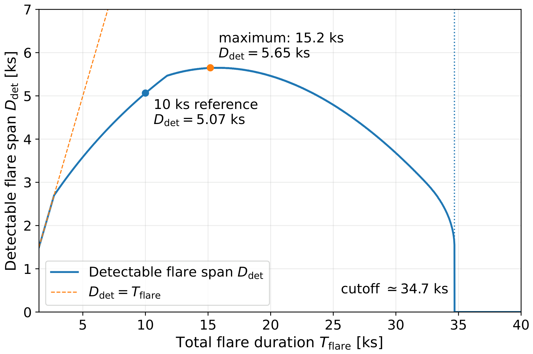
Figure 1 shows the resulting dependence on total flare duration. At the shortest tested duration, $T_{\mathrm{flare}}=1.5$ ks, the complete flare is detectable and $D_{\det }=T_{\mathrm{flare}}$. The detectable span initially grows approximately together with the total flare duration; in the adopted profile the complete flare remains within the detectable span up to approximately 2.7 ks. At longer durations, increasing portions of the low-luminosity parts of the flare no longer belong to any successful 1500 s detection interval, and $D_{\det }$ therefore grows more slowly than $T_{\mathrm{flare}}$.

The detectable span reaches a maximum of approximately $D_{\det }=5.65$ ks at $T_{\mathrm{flare}}\simeq 15.2$ ks. At still longer durations, the fixed total energy is distributed over an increasingly broad light curve and the energy contained within the brightest 1500 s interval decreases. Consequently, $D_{\det }$ decreases again. Near $T_{\mathrm{flare}}\simeq 34.7$ ks, only approximately one qualifying 1500 s interval remains around the flare maximum; beyond this duration, no 1500 s interval reaches the adopted threshold and $D_{\det }=0$.

The 10 ks reference flare adopted in Equation (5) lies well within the detectable regime and gives $D_{\det }=5.065$ ks. We use this single representative case below to illustrate the separate effect of temporal sampling.

The same fixed-energy experiment can also be used to quantify how the mapping between the 1500 s SXI detection criterion and the total flare energy depends on the assumed flare duration. For a given $T_{\mathrm{flare}}$, we define

$$f_{1500}\left(T_{\mathrm{flare}}\right)={\displaystyle \frac{{\max }_t{E}_{1500}\left(t\right)}{E_{\mathrm{flare}}}},$$

(10)

where $f_{1500}$ is the maximum fraction of the total flare energy contained within any complete 1500 s integration interval. Because the model light curve scales linearly with total flare energy, the minimum total flare energy required for the brightest 1500 s interval to reach the SXI threshold is then

$$E_{\min }\left(T_{\mathrm{flare}}\right)={\displaystyle \frac{E_{1500,\mathrm{th}}}{f_{1500}\left(T_{\mathrm{flare}}\right)}}.$$

(11)

For the adopted 10 ks reference profile, $f_{1500}=0.448$, so that the minimum total flare energy required to satisfy the 1500 s detection criterion is approximately $E_{\min }=1.17\times {10}^{36}$ erg. This is substantially below $E_{\mathrm{char}}=3.5\times {10}^{36}$ erg and further illustrates that $E_{\mathrm{char}}$ is a reference energy scale rather than a strict total-energy detection threshold.

Representative results for a broader range of flare durations are listed in

Table 1. Sensitivity of the mapping between the 1500 s SXI detection criterion and total flare energy to the assumed flare duration. The quantity $f_{1500}$ is the maximum fraction of the total flare energy contained within any complete 1500 s interval, and $E_{\min }$ is the minimum total flare energy required for such an interval to reach the SXI threshold. The final column gives the relative flare-yield factor implied by the cumulative COUP relation $N(>E)\propto E^{-1.2}$, normalized to the 10 ks reference profile. These factors are presented as a separate sensitivity test and are not folded into the primary regional yield intervals.

${\mathit{T}}_{\mathbf{flare}}$ [ks]	${\mathit{f}}_{1500}$	${\mathit{E}}_{\mathbf{min}}$ [erg]	Yield Factor
5	0.721	$7.28\times {10}^{35}$	1.77
10	0.448	$1.17\times {10}^{36}$	1.00
15	0.321	$1.64\times {10}^{36}$	0.67
20	0.249	$2.11\times {10}^{36}$	0.49
30	0.172	$3.06\times {10}^{36}$	0.32
40	0.131	$4.01\times {10}^{36}$	0.23
50	0.106	$4.96\times {10}^{36}$	0.18

. As the flare duration increases, a progressively smaller fraction of the total energy is concentrated within the brightest 1500 s interval, and the corresponding minimum detectable total energy therefore increases.

The transition around $T_{\mathrm{flare}}\simeq 34.7$ ks found in the fixed-$E_{\mathrm{char}}$ experiment can now be interpreted directly in terms of this duration-dependent total-energy threshold. At 30 ks, $E_{\min }\simeq 3.06\times {10}^{36}$ erg remains below the adopted $E_{\mathrm{char}}=3.5\times {10}^{36}$ erg, whereas at 40 ks the required energy has increased to $E_{\min }\simeq 4.01\times {10}^{36}$ erg, which exceeds $E_{\mathrm{char}}$. The previously identified ∼34.7 ks limit therefore marks only the point at which the adopted fixed-energy test flare ceases to satisfy the SXI criterion; it does not represent a physical upper limit on the duration of detectable flares. Longer flares remain detectable provided that their total energies are correspondingly larger.

Using the cumulative COUP flare-energy distribution, $N(>E)\propto E^{-1.2}$, the duration-dependent change in the total-energy threshold can be expressed relative to the 10 ks reference profile as

$$C_{\mathrm{dur}}\left(T_{\mathrm{flare}}\right)={\left[{\displaystyle \frac{E_{\min }\left(T_{\mathrm{flare}}\right)}{E_{\min }\left(10\mathrm{ks}\right)}}\right]}^{-1.2}.$$

(12)

For the representative durations in Table 1, this factor ranges from 1.77 at 5 ks to 0.18 at 50 ks. These values quantify the sensitivity of the inferred absolute flare yield to the adopted temporal profile under the fixed total-energy-distribution approximation.

Importantly, this duration dependence does not alter the Orion-relative distance scaling if the same flare-duration and temporal-profile distribution is assumed for all regions. For a given profile,

$$E_{\min ,\mathrm{reg}}\left(T_{\mathrm{flare}}\right)={\Theta }_d{E}_{\min ,\mathrm{Orion}}\left(T_{\mathrm{flare}}\right),$$

(13)

so that the duration-dependent factor is common to Orion and to the comparison region. It therefore affects the absolute yield normalization but not the relative distance scaling or the regional ranking within the present framework. We do not fold this additional sensitivity factor into the primary regional yield intervals, both to keep it distinct from the uncertainty in the absolute Orion flare-rate normalization and because a fully population-based correction would require the joint distribution of flare energy, duration, and temporal profile.

The finite duration of a flare also changes the range of flare onset times that can result in a detection during an individual SXI visit. We illustrate this effect only for the adopted 10 ks reference flare, rather than attempting to reconstruct the unknown THESEUS observing cadence.

For this profile, the detectable portion of the flare extends over $D_{\det }=5.065$ ks and begins at flare onset. The latest successful 1500 s integration can therefore begin $5.065-1.500=3.565$ ks after flare onset. A flare beginning up to 3.565 ks before the start of an SXI visit can consequently still provide a complete detectable 1500 s interval after the visit begins. At the opposite edge, the flare must begin at least 1.5 ks before the visit ends for such an interval to fit within the observation.

For this specific reference profile, the net enlargement of the allowed flare-onset interval is therefore

$$T_{\mathrm{corr}}=D_{\det }-2t_{\mathrm{int}}=5.065-2\left(1.500\right)=2.065\mathrm{ks},$$

(14)

where $t_{\mathrm{int}}=1.5$ ks. An isolated visit of duration $T_{\mathrm{visit}}$ therefore corresponds to an effective flare-onset interval

$$T_{\mathrm{eff}}=T_{\mathrm{visit}}+T_{\mathrm{corr}},$$

(15)

with the illustrative temporal-overlap factor

$$C_{\mathrm{overlap}}={\displaystyle \frac{T_{\mathrm{eff}}}{T_{\mathrm{visit}}}}.$$

(16)

Representative values are listed in

Table 2. Illustrative temporal-overlap effect for the 10 ks reference flare. $T_{\mathrm{eff}}$ is the width of the range of possible flare onset times that can lead to a successful detection during an isolated visit; it is not an increase in the actual instrumental exposure time. $C_{\mathrm{overlap}}$ gives the ratio of this onset-time interval to $T_{\mathrm{visit}}$.

${\mathit{T}}_{\mathbf{visit}}$ [ks]	${\mathit{T}}_{\mathbf{eff}}$ [ks]	${\mathit{C}}_{\mathbf{overlap}}$
100	102.065	1.02
50	52.065	1.04
20	22.065	1.10
10	12.065	1.21
5	7.065	1.41
2	4.065	2.03

.

The values in Table 2 are illustrative flare-onset windows, not increases in instrumental exposure. Because the published SXI exposure map provides only cumulative exposure and does not specify the duration or spacing of individual visits, the overlap factors cannot be propagated uniquely to mission-level yields and are therefore not included in the regional estimates. They are used only to illustrate the possible magnitude of temporal-sampling effects.

2.3.2. Orion Normalization and Regional Scaling

The Orion benchmark is particularly valuable because the COUP survey monitored 1616 young stars continuously for approximately 9.7 days, producing one of the most complete datasets currently available on YSO X-ray variability [5,14,15]. The survey detected a large sample of flare events, corresponding to average flare frequencies of several tens of flares per star per year when extrapolated over a full year [14].

However, THESEUS is not sensitive to the bulk of the flare population. The luminosity threshold derived above lies near the extreme high-energy tail of the observed flare distribution. In the detailed COUP flare analysis of Favata et al. [15], only 32 exceptionally energetic events were selected for detailed study. These flares reached peak luminosities of order

$$L_{X,\mathrm{peak}}\sim {10}^{31}–{10}^{33}\mathrm{erg}{\mathrm{s}}^{-1},$$

(17)

directly overlapping the luminosity regime relevant for SXI detections at the distance of Orion.

The events analyzed by Favata et al. [15] represent approximately the brightest one percent of the full COUP flare population and demonstrate that flares reaching the luminosity regime relevant for SXI occur in young Orion sources. However, this subsample was selected for detailed flare analysis and does not constitute a complete flux-limited sample defined at the SXI sensitivity threshold. It therefore provides an empirical plausibility check on the relevant flare regime rather than a precise measurement of the SXI-detectable flare frequency.

We therefore retain

$$R_{\mathrm{flare},\mathrm{Orion}}=1\mathrm{flare}{\mathrm{source}}^{-1}{\mathrm{yr}}^{-1}$$

(18)

as the fiducial normalization of the model. Since the available COUP samples do not provide a complete SXI-equivalent flux-limited measurement of this rate, we do not interpret this value as a precise empirical determination. Instead, to explicitly assess the sensitivity of the predicted yields to the normalization, we consider the broader range

$$R_{\mathrm{flare},\mathrm{Orion}}=0.2–2\mathrm{flare}{\mathrm{source}}^{-1}{\mathrm{yr}}^{-1}.$$

(19)

This range is adopted as a sensitivity interval around the fiducial value, rather than as a formal statistical confidence interval. Since the predicted flare yields scale linearly with $R_{\mathrm{flare},\mathrm{Orion}}$, it directly illustrates the uncertainty introduced by the poorly constrained absolute flare-rate normalization.

To extrapolate from Orion to other star-forming regions, we use the observed flare-energy distribution derived from COUP. Caramazza et al. [14] showed that the high-energy tail follows a power-law distribution

$${\displaystyle \frac{dN}{dE}}\propto E^{-\alpha },\alpha \simeq 2.2.$$

(20)

The corresponding cumulative distribution is

$$N(>E)\propto E^{-(\alpha -1)}\propto E^{-1.2}.$$

(21)

For the fiducial slope, this relation implies that increasing the flare energy by one decade reduces the cumulative occurrence rate by a factor of ${10}^{1.2}\simeq 16$.

The slope of the flare distribution is itself observationally uncertain. Caramazza et al. [14] obtained $\alpha -1=1.2\pm 0.2$ for the high-count power-law tail of the COUP flare distribution, corresponding to $\alpha =2.2\pm 0.2$. We therefore retain their best-fitting value $\alpha =2.2$ for the primary regional yield estimates and separately examine the corresponding range $\alpha =2.0$–$2.4$ as a sensitivity test. This uncertainty becomes increasingly important when the flare distribution is extrapolated far from the Orion reference threshold. The sensitivity test quantifies the effect of the observationally determined slope uncertainty on the relative extrapolation from Orion to other regions, while the uncertainty in the absolute Orion flare rate is treated independently through the $0.2$–$2{\mathrm{yr}}^{-1}$ normalization interval.

Because the observable flux decreases as $d^{-2}$, the luminosity threshold increases with distance according to

$$L_{\mathrm{th}}\propto d^2.$$

(22)

For convenience, we define the Orion-relative luminosity-threshold factor

$${\Theta }_d={\left({\displaystyle \frac{d_{\mathrm{reg}}}{d_{\mathrm{Orion}}}}\right)}^2,$$

(23)

which expresses how much more luminous a flare must be to remain detectable relative to Orion. Using the COUP flare-energy distribution, this translates into a flare-rate suppression factor

$${\mathrm{\Phi }}_d\left(\alpha \right)={\Theta }_d^{\alpha -1}.$$

(24)

For the fiducial $\alpha =2.2$ adopted in the primary yield calculation, this reduces to

$${\mathrm{\Phi }}_d={\Theta }_d^{1.2}.$$

(25)

The detectable flare rate in a given region is then

$$R_{\mathrm{flare},\mathrm{reg}}={\displaystyle \frac{R_{\mathrm{flare},\mathrm{Orion}}}{{\mathrm{\Phi }}_d}}.$$

(26)

For each region, the adopted range in $R_{\mathrm{flare},\mathrm{Orion}}$ is propagated directly through this relation, so that the resulting flare-yield interval includes the uncertainty associated with the absolute Orion normalization.

Finally, the model-estimated number of flares during the nominal four-year THESEUS mission is calculated as

$$N_{\mathrm{flare},\mathrm{reg}}=N_{\mathrm{eff},\mathrm{reg}}{R}_{\mathrm{flare},\mathrm{reg}}{T}_{\mathrm{mission}},$$

(27)

where $N_{\mathrm{eff},\mathrm{reg}}$ is the exposure-weighted effective number of monitored YSOs and $T_{\mathrm{mission}}=4$ yr. This framework provides a simple Orion-normalized method for comparing the relative THESEUS flare yields across a broad range of Galactic star-forming regions. The resulting values are intended as model-dependent, order-of-magnitude estimates and should not be interpreted as precise event-rate predictions.

2.4. Approximate Effect of X-Ray Absorption

The distance scaling adopted above neglects X-ray absorption along the line of sight. Since the SXI operates in the 0.3–5 keV band, this effect may be significant, particularly for embedded or strongly obscured YSOs. To estimate its magnitude, we performed a representative absorption sensitivity test using XSPEC with a TBabs∗APEC model. We adopted thermal-plasma temperatures of $kT=4$, 8, and 12 keV, corresponding to approximately 46, 93, and 139 MK, respectively. These values span the temperature range relevant to the powerful COUP flares analyzed by Favata et al. [15]. A plasma abundance of $Z=0.3Z_{\odot }$ was adopted, consistent with the coronal abundance used for the flare component by Favata et al. [15], while the absorbing column was modeled with TBabs using the Wilms et al. abundances [16].

We considered representative hydrogen-equivalent column densities of $N_{\mathrm{H}}={10}^{21}$, ${10}^{22}$, and ${10}^{23}$ cm⁻² and calculated the transmitted 0.3–5 keV energy flux relative to the unabsorbed model,

$$T\left(N_{\mathrm{H}}\right)={\displaystyle \frac{F_{\mathrm{absorbed}}}{F_{\mathrm{unabsorbed}}}}.$$

(28)

The resulting transmission factors are listed in

Table 3. Effect of X-ray absorption on the 0.3–5 keV flux for representative thermal flare spectra. The transmission is defined as $T=F_{\mathrm{absorbed}}/F_{\mathrm{unabsorbed}}$. The threshold and flare-yield factors are given for the fiducial $kT=8$ keV model.

${\mathit{N}}_{\mathbf{H}}$ [cm−2]	${\mathit{T}}_{4\mathbf{keV}}$	${\mathit{T}}_{8\mathbf{keV}}$	${\mathit{T}}_{12\mathbf{keV}}$	Threshold Factor	Yield Factor
${10}^{21}$	0.838	0.865	0.875	1.16	0.84
${10}^{22}$	0.516	0.577	0.600	1.73	0.52
${10}^{23}$	0.169	0.213	0.230	4.69	0.16

. For the fiducial $kT=8$ keV model, $86.5\%$, $57.7\%$, and $21.3\%$ of the unabsorbed SXI-band flux remains at $N_{\mathrm{H}}={10}^{21}$, ${10}^{22}$, and ${10}^{23}$ cm⁻², respectively. The corresponding intrinsic detection threshold therefore increases by factors of 1.16, 1.73, and 4.69, respectively. Using the cumulative flare-energy distribution in Equation (21), these values correspond to approximate flare-yield factors of 0.84, 0.52, and 0.16, respectively, relative to the absorption-free case.

The inferred attenuation depends only moderately on the assumed flare temperature over the tested $kT=4$–12 keV range, whereas the dependence on $N_{\mathrm{H}}$ is substantial. Repeating the calculation with solar rather than $0.3Z_{\odot }$ plasma abundance produced negligible changes in the transmission factors. This is expected for such hot flare plasmas, the X-ray spectra of which are dominated by continuum emission and are therefore only weakly sensitive to the adopted metal abundance [15].

To assess whether region-to-region differences in absorption could materially affect the comparative flare-yield predictions, we performed an additional homogeneous line-of-sight sensitivity test. For the same representative coordinates used in the SXI exposure-map analysis (

Table A1. Representative sampling positions, cumulative SXI exposure values, and numerical digitization uncertainties for the target star-forming regions. Coordinates are given in equatorial J2000 degrees. The quoted uncertainty bounds correspond to the 16th and 84th percentiles obtained by combining the valid pixels within the local $5\times 5$ sampling region with independent $\pm 1$ pixel perturbations of the two color-bar calibration anchors. These intervals characterize the numerical sensitivity of the digitization procedure and are not formal confidence intervals on the mission exposure prediction.

Region	RA [deg]	Dec [deg]	SXI Exposure [Days]	Digitization Uncertainty [Days]
Upper Sco	240.00	−23.00	39.91	$-0.29/+0.20$
Orion	83.75	−5.38	52.65	$-0.87/+0.16$
Taurus	68.00	24.00	34.70	$-0.15/+0.29$
$\rho$ Oph	246.75	−24.00	41.36	$-0.20/+0.29$
Lupus	241.00	−39.00	43.39	$-0.39/+0.10$
CrA	285.25	−37.00	39.33	$-0.29/+0.20$
NGC 6334	260.17	−35.83	43.10	$-0.21/+0.39$
Cygnus X	308.25	41.00	67.41	$-0.52/+0.76$
Perseus	56.00	32.00	37.89	$-0.21/+0.21$
Cha I	166.50	−77.00	3.45	$-0.32/+0.90$
Serpens	277.50	1.00	45.41	$-0.30/+1.92$
W40	277.75	−2.00	44.25	$-0.29/+0.39$
Cep OB3	344.00	62.00	8.95	$-0.29/+4.34$
NGC 2264	100.25	9.88	41.94	$-1.25/+0.20$
Mon R2	91.75	−6.38	50.77	$-0.37/+1.05$
Vela	130.00	−43.00	63.06	$-0.16/+0.58$
CMa OB1/R1	105.00	−11.50	47.15	$-0.18/+0.18$
Rosette	97.75	4.93	46.57	$-0.58/+0.18$
NGC 6357	261.39	−34.39	42.52	$-0.20/+0.48$
Carina	161.25	−59.00	13.00	$-0.58/+0.87$

), we obtained the total Galactic hydrogen column density using the $N_{\mathrm{H},\mathrm{tot}}$ framework of Willingale et al. [17], which combines the atomic and molecular hydrogen contributions to estimate the total X-ray absorbing column along a given Galactic line of sight. We adopted the inverse-angular-distance-weighted values returned by the corresponding all-sky implementation, in which nearby map samples within $1°$ of the input coordinate contribute with larger weights.

For each representative line of sight, the resulting $N_{\mathrm{H},\mathrm{tot}}^{\mathrm{LOS}}$ value was applied to the same fiducial $kT=8$ keV, $Z=0.3Z_{\odot }$ TBabs∗APEC model used above. The corresponding absorption-induced flare-yield factor is

$$C_{\mathrm{abs}}=T{\left(N_{\mathrm{H}}\right)}^{\alpha -1}=T{\left(N_{\mathrm{H}}\right)}^{1.2},$$

(29)

where $T\left(N_{\mathrm{H}}\right)$ is the transmitted SXI-band flux fraction and the second equality adopts the fiducial COUP slope $\alpha =2.2$. The resulting region-by-region sensitivity factors are listed in

Table 4. Region-dependent X-ray absorption sensitivity using homogeneous full-Galactic line-of-sight hydrogen columns. Distances are those adopted in the regional flare-yield calculation. $N_{\mathrm{H},\mathrm{tot}}^{\mathrm{LOS}}$ is the inverse-angular-distance-weighted total Galactic hydrogen column obtained at the representative region coordinates using the method of Willingale et al. [17]. $T_{8\mathrm{keV}}$ is the transmitted 0.3–5 keV energy-flux fraction for the fiducial $kT=8$ keV, $Z=0.3Z_{\odot }$ TBabs∗APEC model, and $C_{\mathrm{abs}}$ is the corresponding multiplicative flare-yield factor from Equation (29). The full-line-of-sight columns are used only as a homogeneous sensitivity scenario and are not interpreted as source-specific foreground absorption corrections.

Region	d [pc]	${\mathit{N}}_{\mathbf{H},\mathbf{tot}}^{\mathbf{LOS}}$ [cm−2]	${\mathit{T}}_{8\mathbf{keV}}$	${\mathit{C}}_{\mathbf{abs}}$
Upper Sco	145	$1.71\times {10}^{21}$	0.810	0.777
Orion	414	$3.13\times {10}^{21}$	0.738	0.694
Taurus	140	$2.92\times {10}^{21}$	0.747	0.704
$\rho$ Oph	137	$2.79\times {10}^{21}$	0.752	0.711
Lupus	175	$2.89\times {10}^{21}$	0.748	0.706
CrA	135	$1.55\times {10}^{21}$	0.821	0.789
NGC 6334	1760	$1.40\times {10}^{22}$	0.527	0.463
Cygnus X	1400	$1.29\times {10}^{22}$	0.539	0.477
Perseus	300	$2.59\times {10}^{21}$	0.761	0.721
Cha I	190	$2.07\times {10}^{21}$	0.788	0.752
Serpens	430	$5.34\times {10}^{21}$	0.667	0.615
W40	500	$7.29\times {10}^{21}$	0.623	0.567
Cep OB3	700	$1.02\times {10}^{22}$	0.574	0.514
NGC 2264	760	$5.40\times {10}^{21}$	0.665	0.613
Mon R2	830	$3.72\times {10}^{21}$	0.715	0.669
Vela	850	$1.11\times {10}^{22}$	0.562	0.501
CMa OB1/R1	1000	$7.90\times {10}^{21}$	0.612	0.554
Rosette	1600	$7.52\times {10}^{21}$	0.619	0.562
NGC 6357	1760	$1.37\times {10}^{22}$	0.530	0.467
Carina	2300	$1.21\times {10}^{22}$	0.549	0.487

.

Importantly, the tabulated $N_{\mathrm{H},\mathrm{tot}}^{\mathrm{LOS}}$ values are integrated through the full Galactic line of sight and should not be interpreted as measurements of the actual foreground column toward the YSOs in each region. In particular, part of the mapped column may lie behind a nearby star-forming region, while small-scale cloud structure and local or circumstellar absorption toward individual embedded sources are not necessarily represented by the large-scale all-sky estimate. The region distance is therefore included in Table 4 as interpretive context only; we do not assume a uniform spatial distribution of the absorbing material or use distance to assign a foreground fraction. Instead, the calculation represents an illustrative full-line-of-sight screen scenario for the mapped Galactic component.

The homogeneous line-of-sight test shows a systematic but moderate regional dependence. For the nearby regions extending from CrA at 135 pc to Orion at 414 pc, the full-Galactic columns at the adopted representative positions are only $N_{\mathrm{H},\mathrm{tot}}^{\mathrm{LOS}}\simeq (1.55$–$3.13)\times {10}^{21}$ cm⁻², corresponding to yield factors of approximately 0.69–0.79 even in the full-line-of-sight screen scenario. By contrast, several of the distant massive star-forming complexes have substantially larger full-line-of-sight columns: NGC 6334, Cygnus X, NGC 6357, and Carina have $N_{\mathrm{H},\mathrm{tot}}^{\mathrm{LOS}}\simeq (1.21$–$1.40)\times {10}^{22}$ cm⁻², with corresponding factors of approximately 0.46–0.49.

Across the complete regional sample, the full-line-of-sight sensitivity factors span $C_{\mathrm{abs}}=0.463$–0.789. Thus, the maximum differential change in the relative yield of two regions within this homogeneous scenario is approximately

$${\displaystyle \frac{0.789}{0.463}}\simeq 1.70.$$

(30)

Absorption can therefore modify the ordering of regions whose absorption-free predictions are intrinsically similar, but this representative test does not overturn the broader comparative trend favoring nearby regions over more distant, high-column directions.

More extreme differences remain possible for individual embedded sources. Using the generic absorption scenarios in Table 3, the unrounded model values imply differential relative-yield changes of approximately 1.62 between $N_{\mathrm{H}}={10}^{21}$ and ${10}^{22}$ cm⁻², 3.31 between ${10}^{22}$ and ${10}^{23}$ cm⁻², and 5.37 between ${10}^{21}$ and ${10}^{23}$ cm⁻²; the contrast between an unabsorbed source and $N_{\mathrm{H}}={10}^{23}$ cm⁻² is approximately a factor of 6.4. Thus, sufficiently different source-specific absorption can indeed alter the relative ranking of otherwise comparable targets.

Because homogeneous source-by-source foreground $N_{\mathrm{H}}$ measurements are not available for the heterogeneous YSO samples considered here, we do not apply the factors in Table 4 as corrections to the primary regional flare-yield intervals. The absorption-free predictions should instead be regarded as optimistic baseline estimates, while Table 3 and Table 4 separately quantify the possible magnitude of generic and region-dependent absorption effects.

2.5. SXI Exposure-Map Analysis

The flare-occurrence framework described above provides a model estimate of the detectable flare rate for a continuously monitored YSO population. In practice, however, individual star-forming regions are observed only intermittently during the THESEUS survey. The probability of detecting a flare therefore depends not only on the intrinsic flare frequency but also on the temporal sampling of a given region. In the absence of a detailed mission timeline, we approximate this sampling using the cumulative exposure received by each region over the mission lifetime.

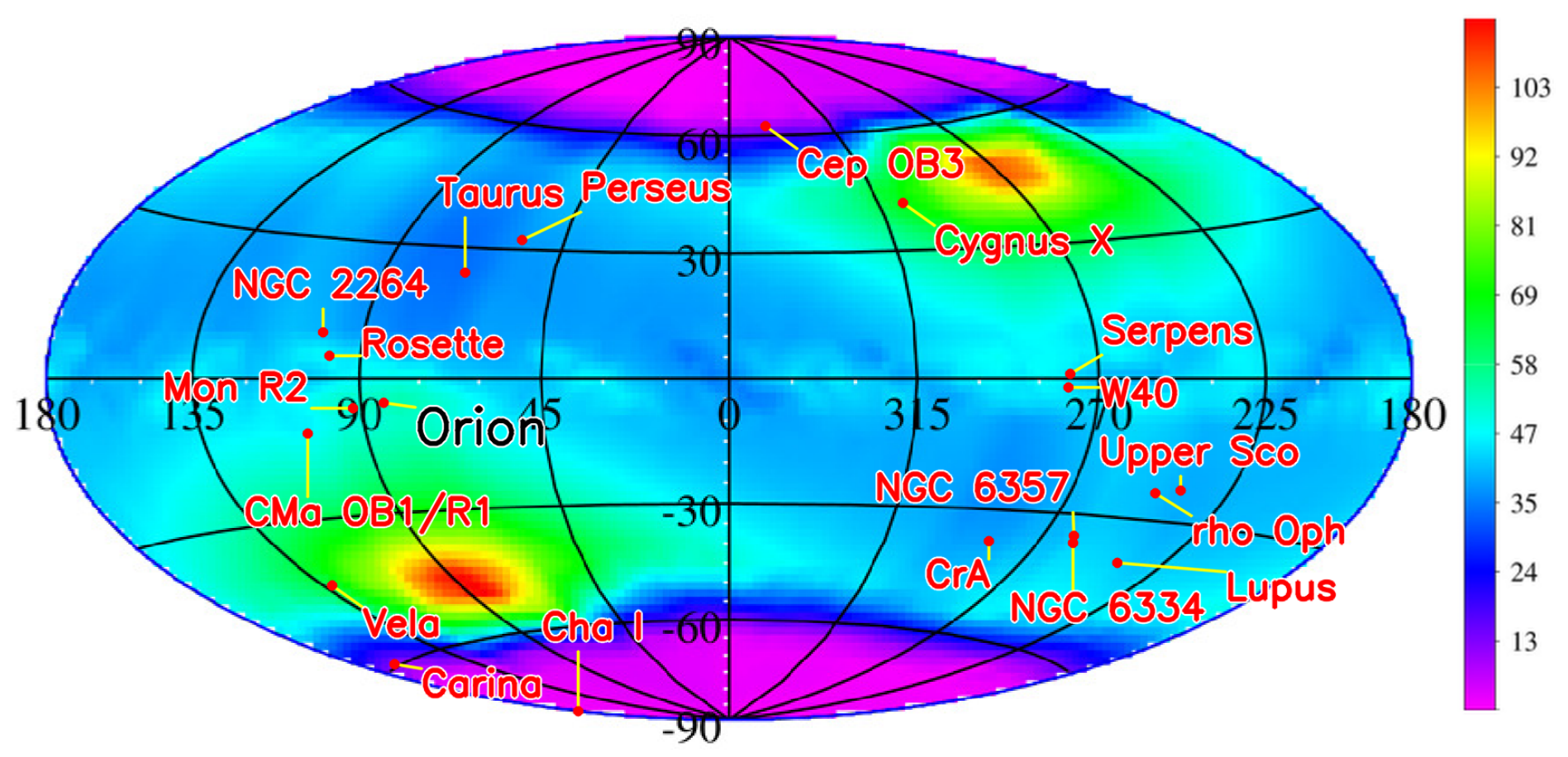
To quantify this effect, we used the all-sky SXI exposure map provided in the THESEUS Yellow Book. The map describes the cumulative exposure expected under the nominal Dynamic (DYN) pointing strategy and reveals substantial spatial variations in sky coverage. While some regions are observed for more than 100 days over the nominal mission lifetime, others receive fewer than 10 days of total exposure.

For each star-forming region considered in this study, the cumulative SXI exposure time $t_{\exp }$ was extracted from the THESEUS all-sky exposure map. The technical details of the map digitization, coordinate transformation, and color-scale calibration are described in Appendix A. The adopted exposure map and the locations of the analyzed star-forming regions are shown in Figure A1.

Because the exposure values are extracted from a published graphical map rather than from a machine-readable dataset, they are subject to a small numerical digitization uncertainty. This uncertainty was quantified from the local pixel variation and the finite precision of the color-scale calibration; the procedure and region-by-region uncertainty intervals are given in Appendix A.

The exposure information was converted into a coverage fraction

$$f_{\mathrm{cov}}={\displaystyle \frac{t_{\exp }}{T_{\mathrm{mission}}}},$$

(31)

where $T_{\mathrm{mission}}=1461$ days corresponds to the nominal four-year mission lifetime.

This treatment represents a first-order temporal-coverage approximation. The cumulative exposure map provides the total observing time at a given sky position, but does not specify the number, duration, spacing, or temporal sequence of the individual SXI observing intervals. As demonstrated in Section 2.3.1, the adopted 10 ks reference flare produces an additional flare-onset overlap window relative to the instantaneous-event approximation, and the magnitude of this effect depends strongly on how the cumulative exposure is divided among individual visits. Since the detailed visit sequence is not available, no unique mission-level correction can be derived, and we therefore retain Equation (31) for the primary regional calculations.

Within the instantaneous-event approximation used for the primary yield calculation, the coverage fraction represents the probability that a randomly occurring event falls within the accumulated SXI observing time. Consequently, the observable fraction is approximated by $f_{\mathrm{cov}}$.

To account for this effect, we define an effective monitored population

$$N_{\mathrm{eff}}=N_{\mathrm{YSO}}{f}_{\mathrm{cov}},$$

(32)

where $N_{\mathrm{YSO}}$ is the adopted YSO population of the region. The quantity $N_{\mathrm{eff}}$ can be interpreted as the number of continuously monitored YSOs that would produce the same expected number of detections as the actual intermittently observed population.

The model-estimated number of detectable flares is then obtained by combining $N_{\mathrm{eff}}$ with the distance-dependent flare-rate formalism described in Section 2.3. This approach provides a simple and physically intuitive framework for comparing regions that differ simultaneously in stellar population, sky position, and cumulative THESEUS exposure.

2.6. IRT Source-Separation Analysis

While the SXI determines whether a flare can be detected, the scientific interpretation of such events also depends strongly on source crowding in IRT observations. We therefore evaluated nearest-neighbor source-separation statistics in representative low- and high-density star-forming regions.

The analysis is based on the expected imaging performance of the IRT as reported in the THESEUS Yellow Book. Adopting the planned optical performance of the IRT (${\theta }_{\mathrm{EE}50}<{1.28}^{″}$ and ${\theta }_{\mathrm{EE}80}<{2.29}^{″}$, corresponding to the diameters enclosing 50% and 80% of the point-spread-function energy, respectively), we classify sources according to their angular separation from the nearest neighbor. We distinguish sources with separations below the EE50 scale ($<{1.28}^{″}$), between the EE50 and EE80 scales (${1.28}^{″}$–${2.29}^{″}$), and beyond the EE80 scale ($>{2.29}^{″}$). These categories characterize angular source separation relative to the expected IRT point-spread function and should not be interpreted as strict photometric deblending limits. Actual photometric recoverability will additionally depend on source contrast, signal-to-noise ratio, background level, and the adopted extraction method.

For nearby star-forming regions, we use the Orion Nebula Cluster as a benchmark. Source positions were taken from the NEMESIS catalog [18], and nearest-neighbor statistics were computed for all objects within the analyzed field. To evaluate the robustness of the results under more extreme crowding conditions, we additionally generated a synthetic stress-test population by increasing the source density by a factor of five while preserving the overall spatial distribution.

For more distant and more heavily populated environments such as the Carina Nebula Complex (CNC), complete source catalogs are not available across the full region at the required level of membership reliability. In this case, a statistical approach was adopted. Using published source counts and survey areas, the projected source density was estimated and the probability of source isolation was calculated assuming a two-dimensional Poisson point process. The Poisson treatment is intended as a baseline description of the projected line-of-sight source field and should not be interpreted as a physical model in which the young Carina population itself is spatially unclustered. The full infrared source sample contains a large population of unrelated field sources in addition to members of the star-forming complex, whereas the latter are known to be strongly clustered. The effect of a compact young stellar concentration is therefore considered separately below using Trumpler 14 as a dense-cluster benchmark. For the approximately uniform projected field population, the probability that a source has no neighbor within angular distance R is given by

$$P(d>R)=\exp (-\pi R^2\sigma ),$$

(33)

where $\sigma$ is the projected source density.

This Poisson expression is used as a baseline description of the global CNC field. To assess the additional effect of clustering, we performed a separate Monte Carlo stress test for a $2^{\prime }\times 6^{\prime }$ area corresponding to the combined footprint of three $2^{\prime }\times 2^{\prime }$ IRT Guest Observer windows. The underlying projected field population was scaled from the source density measured by Preibisch et al. [13], and an additional mildly centrally concentrated Trumpler 14 component was superposed on this field. This construction is intended as an illustrative crowding test rather than as a detailed structural model of the cluster.

It is important to note that this analysis addresses angular source separation relative to the adopted IRT EE50 and EE80 scales and does not constitute a direct assessment of photometric recoverability or imply unique flare-source identification from SXI detections. The $\sim 2^{\prime }$ localization accuracy of SXI is generally sufficient for placing an event within the ${15}^{\prime }\times {15}^{\prime }$ IRT field of view, but is often insufficient to identify a unique counterpart in dense star-forming regions. Source identification therefore depends both on IRT source-separation performance and on the number of candidate counterparts within the SXI localization region.

3. Results

3.1. Orion Benchmark

The Orion Molecular Cloud Complex serves as the primary nearby benchmark throughout this work. Its proximity, rich young stellar population, and extensive X-ray and infrared observational coverage make it the most suitable reference region for evaluating the YSO science potential of THESEUS.

Using the framework described in Section 2.3, Orion defines the reference case for the flare-yield calculation. The adopted YSO population of the complex is $N_{\mathrm{YSO}}=4000$–8000, while the SXI exposure-map analysis gives a cumulative exposure of 52.65 days over the nominal four-year mission. This corresponds to a coverage fraction of

$$f_{\mathrm{cov}}=0.036,$$

(34)

and therefore to an effective monitored population of

$$N_{\mathrm{eff}}\approx 145–290.$$

(35)

Since Orion is the reference region, the distance-dependent factors are ${\Theta }_d=1$ and ${\mathrm{\Phi }}_d=1$. Using the $0.2$–$2{\mathrm{yr}}^{-1}$ Orion flare-rate sensitivity interval introduced in Section 2.3, the resulting model estimate for the number of SXI-detectable YSO flares during the nominal mission lifetime is

$$N_{\mathrm{flare},\mathrm{Orion}}\approx 100–2350.$$

(36)

Thus, Orion represents the clearest case in which THESEUS can provide a substantial sample of high-energy YSO flares. Because Orion defines the reference threshold itself, varying $\alpha$ does not modify this interval: the slope sensitivity affects only the extrapolation from Orion to regions with different luminosity thresholds.

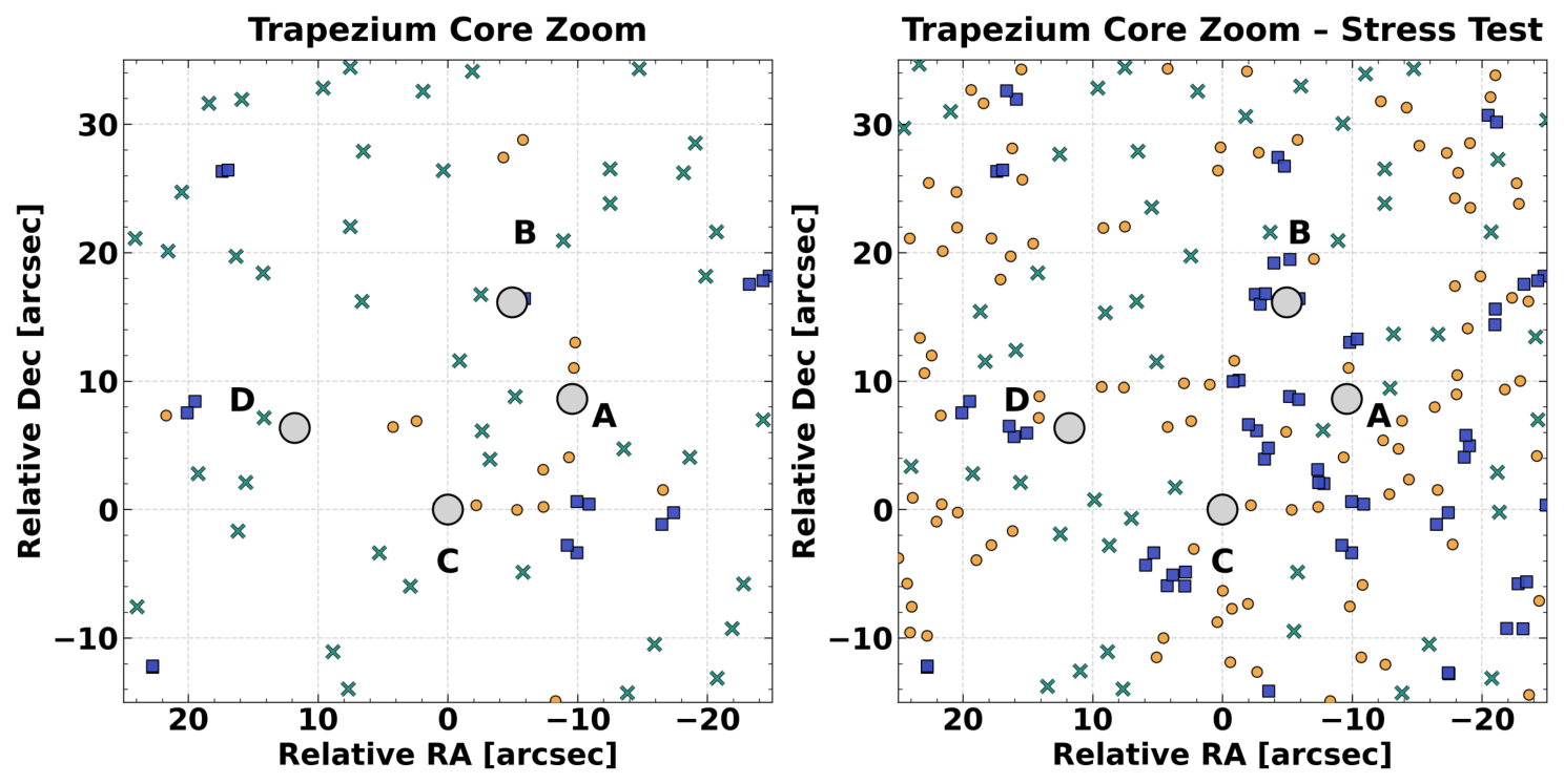
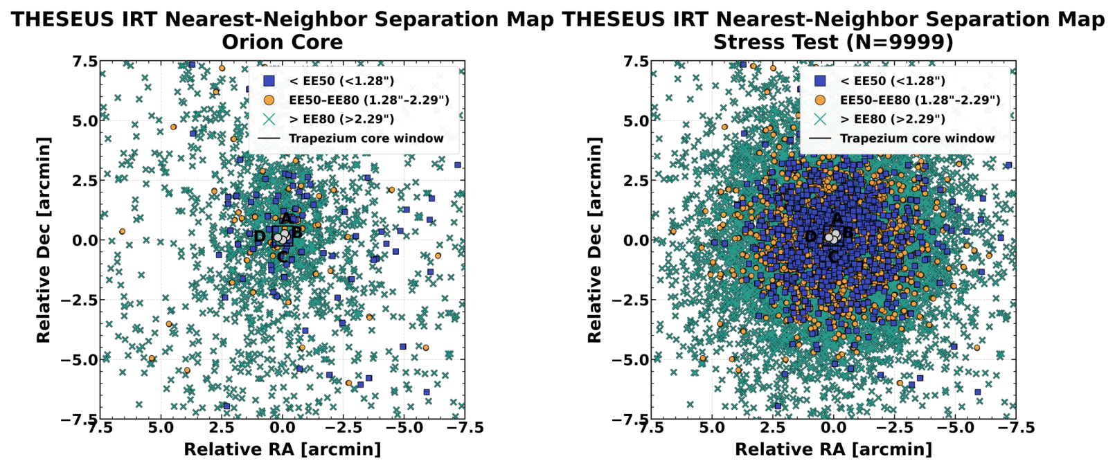
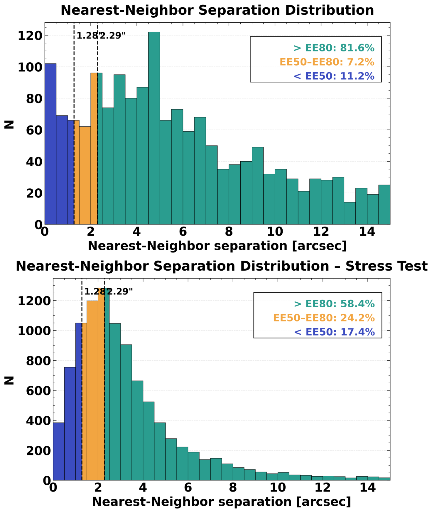
The Orion field also provides a direct test of nearest-neighbor source separations relative to the adopted IRT EE scales using real source positions. We analyzed 1891 cataloged YSOs from the NEMESIS catalog [18] located within a ${15}^{\prime }\times {15}^{\prime }$ field centered on the Trapezium cluster, corresponding to the nominal field of view of the IRT, and computed nearest-neighbor separations for each source. Approximately $81.6\%$ of the sources have nearest-neighbor separations larger than the adopted ${\theta }_{\mathrm{EE}80}={2.29}^{″}$ angular scale. Sources with separations between ${1.28}^{″}$ and ${2.29}^{″}$ fall between the adopted EE50 and EE80 scales, while only a smaller fraction have nearest-neighbor separations below the ${1.28}^{″}$ EE50 scale.

The spatial distribution of the adopted nearest-neighbor separation categories is shown in Figure 2. Even in the dense Trapezium region, shown in Figure 3, nearly half of the sources have nearest-neighbor separations larger than the adopted ${2.29}^{″}$ EE80 scale. The corresponding nearest-neighbor distributions are shown in Figure 4.

To test whether this conclusion remains valid under substantially stronger crowding, we constructed a stress-test population by retaining the complete original NEMESIS-based Orion sample and adding synthetic sources until the total population reaches $N=9999$ objects. This corresponds to an approximately five-fold increase in source density relative to the original sample. As expected, the additional sources shift the nearest-neighbor distribution toward smaller separations and increase the fraction of sources falling below the adopted EE-based separation scales. Nevertheless, even in this extreme artificial case, $58.4\%$ of the sources retain nearest-neighbor separations larger than the ${2.29}^{″}$ EE80 scale. The corresponding fractions in all three EE-based separation categories for both the nominal and stress-test samples are shown in Figure 4.

These results indicate that angular source separation alone does not exclude source-level IRT analysis for a large fraction of an Orion-like population. They do not, however, constitute a direct photometric deblending test. A large fraction of the young stellar population retains angular separations larger than the adopted EE-based scales, even in dense cluster cores and under substantially increased crowding conditions, although actual photometric deblending will depend on additional observational factors.

3.2. Carina Benchmark

While Orion represents a nearby benchmark, the Carina Nebula Complex (CNC) probes the opposite extreme of parameter space. At a distance of approximately 2.3 kpc [12], Carina contains one of the richest young stellar populations in the Galaxy and provides a representative example of a distant, massive, and highly crowded star-forming environment.

To evaluate source crowding, we first consider the deep near-infrared survey of Preibisch et al. [13], which identified approximately $6\times {10}^5$ infrared sources within a central ${36}^{\prime }\times {36}^{\prime }$ field. This number represents the full infrared source population detected in the field and should not be interpreted as the number of YSOs; it is used here only to assess source crowding. Applying the Poisson framework described in Section 2.6 yields

$$P(d>{1.28}^{″})\approx 0.51,$$

(37)

indicating that roughly half of the sources in the global CNC field have nearest-neighbor separations larger than the adopted EE50 scale.

We further examined the dense Trumpler 14 region as a stress test of the effect of clustered young stars on the global CNC crowding estimate. We considered a $2^{\prime }\times 6^{\prime }$ field, corresponding to the combined footprint of three $2^{\prime }\times 2^{\prime }$ IRT Guest Observer windows. Scaling the $\sim 6\times {10}^5$ infrared sources detected over the $0.36{\mathrm{deg}}^2$ HAWK-I field of Preibisch et al. [13] to this area gives approximately 5550 projected field sources. These sources were distributed uniformly to reproduce the mean projected source density of the HAWK-I field. This approximation is motivated by the fact that the detected catalog is numerically dominated by line-of-sight foreground and background sources, which are not expected to exhibit the same degree of small-scale clustering as the young CNC population. The approximation is therefore intended only as a first-order baseline description of the projected source field; the contribution of the spatially clustered young population is considered separately below.

To this field we added 1000 synthetic Trumpler 14 members following a mildly centrally concentrated two-dimensional Gaussian distribution with ${\sigma }_x={35}^{″}$ and ${\sigma }_y={100}^{″}$. This component is intended as a plausible clustering stress test rather than a detailed structural model of Trumpler 14, allowing us to assess how clustering changes the nearest-neighbor statistics relative to the global projected-field baseline.

Across 500 Monte Carlo realizations, the projected field alone gives a mean fraction of $51.8\%$ of sources with nearest-neighbor separations larger than $1.{28}^{″}$, with a realization-to-realization standard deviation of 0.8 percentage points. This is in excellent agreement with the analytic Poisson estimate in Equation (37). After adding the clustered Trumpler 14 component, the corresponding mean fraction decreases to $45.8\%$, with a standard deviation of 0.7 percentage points, for the full simulated source population. Considering only the 1000 synthetic cluster members, the mean fraction is $44.1\%$, with a standard deviation of 1.7 percentage points.

The reduction relative to the global CNC baseline is therefore modest: introducing a clustered young stellar component lowers the fraction beyond the EE50 scale by only about six percentage points. Tests using broader cluster distributions, with $({\sigma }_x,{\sigma }_y)=({45}^{″},{120}^{″})$ and $({60}^{″},{180}^{″})$, yielded full-field fractions of approximately 45.8% and 46.0%, respectively. The result is therefore only weakly sensitive to the precise mild-to-moderate concentration adopted for the synthetic cluster component. These values describe angular source separation only and should not be interpreted as direct predictions of photometric deblending or recovery performance.

A second limitation arises from bright massive stars. Adopting a characteristic contamination radius of approximately ${12}^{″}$ around roughly 200 luminous stars, we estimate that only about 2.2% of the surveyed area is significantly affected by PSF contamination, leaving approximately 98% of the field suitable for high-quality photometry.

The flare-detection prospects of Carina differ substantially from those of Orion. The cumulative SXI exposure toward the CNC is approximately 13 days over the nominal mission lifetime, corresponding to a coverage fraction of

$$f_{\mathrm{cov}}\approx 0.009$$

(38)

Combining this coverage fraction with the separately adopted YSO population of approximately $5\times {10}^4$ members yields an effective monitored population of

$$N_{\mathrm{eff}}\approx 450$$

(39)

In the primary absorption-free baseline calculation, Carina lies roughly 5.5 times farther away than Orion, so the corresponding SXI luminosity threshold increases by a factor of approximately 31. For the fiducial $\alpha =2.2$ flare-energy distribution adopted in Section 2.3, this translates into a reduction of the detectable flare frequency by approximately a factor of 61, yielding

$$R_{\mathrm{flare},\mathrm{Carina}}\approx 0.003–0.033{\mathrm{source}}^{-1}{\mathrm{yr}}^{-1}$$

(40)

The resulting absorption-free baseline model estimate for the number of detectable flares during the nominal four-year mission is therefore

$$N_{\mathrm{flare}}\approx 5–60$$

(41)

Unlike Orion, these detections would probe only the extreme upper tail of the YSO flare-energy distribution. Relative to Orion, the distance-scaled reference energy $E_{\mathrm{char}}{\Theta }_d$ reaches approximately ${10}^{38}$ erg for Carina. As discussed in Section 2.3.1, this quantity is a reference energy scale used for the regional extrapolation rather than a strict total-flare-energy detection threshold; the actual minimum detectable total energy also depends on the flare duration and temporal profile.

This regime should be interpreted with caution. The calculation assumes that the Orion-derived power-law flare-energy distribution remains applicable when extrapolated to substantially higher energies. A physical upper limit must ultimately exist because the magnetic-energy reservoir of a young star is finite, and the distribution may steepen or turn over before this limit is reached. However, neither the location nor the functional form of such a high-energy cutoff is sufficiently constrained for YSOs to justify introducing an additional quantitative cutoff model here. Studies of stellar superflares on late-type stars have reported energies approaching ${10}^{38}$ erg across X-ray, ultraviolet, and optical observations [19], but it remains unclear whether comparable energies can routinely be reached by YSO flares in the X-ray domain.

Carina therefore provides a particularly strong test of the assumed continuation of the flare-energy distribution. A high-energy steepening or cutoff would reduce the predicted yield relative to the simple power-law extrapolation, potentially by a substantial amount. Conversely, detections broadly consistent with the extrapolated rate would provide empirical evidence that the Orion-derived distribution extends into this extreme regime.

Finally, it is important to distinguish angular source separation, photometric deblending, and unique counterpart identification. Although approximately half of the infrared sources are expected to have nearest-neighbor separations larger than the adopted IRT EE50 scale, the $\sim 2^{\prime }$ localization accuracy of SXI generally remains insufficient to uniquely identify a flare-producing object within a dense Carina subcluster. In most cases, SXI detections are therefore expected to localize active regions rather than unique stellar counterparts. Unique source identification would require either simultaneous IRT observations or the occurrence of the flare in a sufficiently sparse environment.

3.3. Model-Estimated Flare Yields

The Orion and Carina benchmark cases illustrate the two ends of the parameter space explored in this work. Orion represents a nearby, well-characterized reference region where the SXI threshold reaches the bright but still empirically motivated part of the YSO flare distribution. Carina, by contrast, represents the distant massive-cluster regime, where only the most extreme high-energy tail of the flare distribution can remain detectable. To extend this comparison to a broader sample of Galactic star-forming regions, we applied the Orion-normalized framework described in Section 2.3 and the SXI exposure-map analysis described in Section 2.5.

The resulting region-by-region flare-yield estimates are summarized in

Table 5. Region-by-region SXI flare-yield estimates normalized to the Orion benchmark. The flare-energy distribution is evaluated at the fiducial COUP slope $\alpha =2.2$, while the Orion flare-rate normalization is varied over $R_{\mathrm{flare},\mathrm{Orion}}=0.2$–$2{\mathrm{yr}}^{-1}$. Exposure times were extracted from the THESEUS all-sky exposure map using the adopted region coordinates. For each region, we list the adopted distance, YSO population, cumulative SXI exposure, coverage fraction $f_{\mathrm{cov}}$, effective monitored population $N_{\mathrm{eff}}$, Orion-relative threshold factor ${\Theta }_d$, fiducial flare-rate suppression factor ${\mathrm{\Phi }}_d$, detectable flare-rate interval $R_{\mathrm{flare},\mathrm{reg}}$, four-year flare-yield interval $N_{\mathrm{flare},\mathrm{reg}}$, and literature sources for the adopted population. The reported intervals are sensitivity ranges rather than formal statistical confidence intervals. The four-year yield intervals are deliberately rounded with a precision appropriate to their magnitude, reflecting their intended use as comparative, order-of-magnitude estimates rather than precise event-rate predictions. The adopted YSO populations are heterogeneous literature-based estimates; their observational or extrapolative basis is summarized in Table A2 in Appendix B. The tabulated yields are the primary absorption-free baseline estimates; flare-duration and temporal-sampling effects are quantified separately in Section 2.3.1, while X-ray absorption is treated separately in Section 2.4.

Region	d [pc]	${\mathit{N}}_{\mathbf{YSO}}$	Days	${\mathit{f}}_{\mathbf{cov}}$	${\mathit{N}}_{\mathbf{eff}}$	${\mathbf{\Theta }}_{\mathit{d}}$	${\mathbf{\Phi }}_{\mathit{d}}$	${\mathit{R}}_{\mathbf{flare},\mathbf{reg}}$ [yr−1]	${\mathit{N}}_{\mathbf{flare},\mathbf{reg}}$/4 yr	Refs.
Upper Sco	145	2000	39.91	0.027	55	0.12	0.08	2.5–24.8	500–5450	[20,21,22]
Orion	414	4000–8000	52.65	0.036	145–290	1.00	1.00	0.20–2.0	100–2350	[5,8,23]
Taurus	140	350–400	34.70	0.024	8–10	0.11	0.07	2.7–27.0	50–1050	[10,24]
$\rho$ Oph	137	150–300	41.36	0.028	4–9	0.11	0.07	2.8–28.4	50–1000	[25]
Lupus	175	150–300	43.39	0.030	5–9	0.18	0.13	1.6–15.8	50–600	[26]
CrA	135	50–100	39.33	0.027	1–3	0.11	0.07	2.9–29.4	10–320	[27]
NGC 6334	1760	20,000–30,000	43.10	0.030	590–885	18.07	32.24	0.006–0.062	10–220	[28,29]
Cygnus X	1400	>10,000	67.41	0.046	460	11.44	18.62	0.011–0.11	10–200	[30,31]
Perseus	300	400	37.89	0.026	10	0.53	0.46	0.43–4.3	10–180	[32,33]
Cha I	190	200–250	3.45	0.002	0.5–0.6	0.21	0.15	1.3–13.0	5–35	[34,35]
Serpens	430	235–300	45.41	0.031	7–9	1.08	1.10	0.18–1.8	5–70	[36,37]
W40	500	600	44.25	0.030	18	1.46	1.57	0.13–1.3	5–95	[29,38]
Cep OB3	700	1000	8.95	0.006	6	2.86	3.53	0.057–0.57	5–15	[39]
NGC 2264	760	1000	41.94	0.029	29	3.37	4.30	0.047–0.47	5–55	[40]
Mon R2	830	300–500	50.77	0.035	10–17	4.02	5.31	0.038–0.38	5–30	[41,42]
Vela	850	>1000	63.06	0.043	43	4.22	5.62	0.036–0.36	5–65	[43]
CMa OB1/R1	1000	300–500	47.15	0.032	10–16	5.83	8.30	0.024–0.24	5–20	[44,45]
Rosette	1600	2000	46.57	0.032	64	14.94	25.65	0.008–0.078	5–20	[46]
NGC 6357	1760	3600–11,000	42.52	0.029	105–320	18.07	32.24	0.006–0.062	5–80	[29,47]
Carina	2300	50,000	13.00	0.009	445	30.86	61.28	0.003–0.033	5–60	[48,49]

.

Because the adopted YSO population values originate from heterogeneous literature surveys and are not based on a uniform census methodology, their observational or extrapolative basis differs among regions. A region-by-region summary of the adopted population basis is provided in

Table A2. Population basis of the YSO numbers adopted for the individual star-forming regions. The terminology summarizes the general observational or extrapolative origin of the population values used in Table 5; the individual literature references are given in that table.

Region	Population Basis
Upper Sco	Astrometric and spectroscopic membership census
Orion	X-ray/IR censuses and broader population estimates
Taurus	Multi-survey membership census with spectroscopy
$\rho$ Oph	Multi-wavelength membership census
Lupus	Spitzer-based multi-wavelength YSO sample
CrA	Multi-wavelength membership sample
NGC 6334	X-ray census with XLF-based extrapolation
Cygnus X	IR-selected samples and regional estimates
Perseus	Spitzer/c2d infrared YSO census
Cha I	Membership census with spectroscopic confirmation
Serpens	Spitzer/c2d IR-selected YSO census
W40	X-ray census with XLF-based population estimate
Cep OB3	X-ray, infrared, and optical membership census
NGC 2264	Multi-wavelength census and population estimate
Mon R2	Near-IR cluster census and population estimate
Vela	Literature-based regional population estimate
CMa OB1/R1	Multi-wavelength membership studies and regional estimates
Rosette	Multi-wavelength population estimate
NGC 6357	Multi-wavelength census and population extrapolation
Carina	X-ray census with total-population extrapolation

in Appendix B.

The largest model-estimated flare yields are obtained for nearby regions with favorable distances and sufficiently large source populations. Upper Scorpius, Taurus, and $\rho$ Ophiuchi all lie within approximately 150 pc and therefore benefit strongly from the distance-dependent scaling, while Orion remains among the most productive regions because of its substantially larger YSO population. At the fiducial $\alpha =2.2$, the adopted $0.2$–$2{\mathrm{yr}}^{-1}$ Orion normalization produces broad but still informative sensitivity intervals: for example, the four-year estimates are approximately 500–5450 flares for Upper Scorpius, 100–2350 for Orion, 50–1050 for Taurus, and 50–1000 for $\rho$ Ophiuchi.

These intervals should not be interpreted as statistical confidence ranges. Their purpose is to show how the absolute normalization uncertainty propagates through an otherwise fixed $\alpha =2.2$ scaling. Within this primary absorption-free baseline, the ranking is strongly distance dependent: exposure time and population size enter linearly, whereas the detectable flare rate scales approximately as $d^{-2.4}$ at the fiducial slope. Consequently, nearby regions are extrapolated toward lower flare energies than the Orion reference threshold, while distant regions require extrapolation toward progressively higher energies.

The uncertainty in the COUP power-law slope is therefore examined separately in

Table 6. Sensitivity of the regional flare-rate scaling to the COUP power-law slope. The entries give the multiplicative change in $R_{\mathrm{flare},\mathrm{reg}}$, and therefore in $N_{\mathrm{flare},\mathrm{reg}}$, for $\alpha =2.0$ and $2.4$ relative to the fiducial $\alpha =2.2$ calculation in Table 5. This test isolates the slope uncertainty in the Orion-to-region extrapolation; uncertainty in the absolute Orion normalization is treated separately through the $0.2$–$2{\mathrm{yr}}^{-1}$ sensitivity interval. The factors follow Equation (24), with Orion remaining unchanged because ${\Theta }_d=1$.

Region	${\mathbf{\Theta }}_{\mathit{d}}$	Factor at $\mathit{\alpha }=2.0$	Factor at $\mathit{\alpha }=2.4$	Overall Factor Range
Upper Sco	0.12	0.66	1.52	0.66–1.52
Orion	1.00	1.00	1.00	1.00–1.00
Taurus	0.11	0.65	1.54	0.65–1.54
$\rho$ Oph	0.11	0.64	1.56	0.64–1.56
Lupus	0.18	0.71	1.41	0.71–1.41
CrA	0.11	0.64	1.57	0.64–1.57
NGC 6334	18.07	1.78	0.56	0.56–1.78
Cygnus X	11.44	1.63	0.61	0.61–1.63
Perseus	0.53	0.88	1.14	0.88–1.14
Cha I	0.21	0.73	1.37	0.73–1.37
Serpens	1.08	1.02	0.98	0.98–1.02
W40	1.46	1.08	0.93	0.93–1.08
Cep OB3	2.86	1.23	0.81	0.81–1.23
NGC 2264	3.37	1.28	0.78	0.78–1.28
Mon R2	4.02	1.32	0.76	0.76–1.32
Vela	4.22	1.33	0.75	0.75–1.33
CMa OB1/R1	5.83	1.42	0.70	0.70–1.42
Rosette	14.94	1.72	0.58	0.58–1.72
NGC 6357	18.07	1.78	0.56	0.56–1.78
Carina	30.86	1.99	0.50	0.50–1.99

. Varying $\alpha$ from 2.0 to 2.4 changes the fiducial regional predictions by multiplicative factors whose magnitude depends on the distance from Orion. The effect is modest for regions with thresholds close to the Orion value, but becomes increasingly important for the nearest and most distant targets. For example, the Upper Scorpius estimate is modified by factors of 0.66–1.52, whereas the Carina estimate is modified by factors of 0.50–1.99. Orion itself is unchanged because it defines the reference threshold, ${\Theta }_d=1$. These factors quantify only the sensitivity of the Orion-to-region extrapolation to the slope uncertainty; they are not folded into the primary intervals in Table 5, in order to keep the effects of the absolute normalization and the extrapolation slope explicitly separated.

The X-ray absorption analysis provides a separate sensitivity test of how line-of-sight attenuation may modify these regional comparisons. In the homogeneous full-Galactic line-of-sight screen scenario of Table 4, the regional yield factors span $C_{\mathrm{abs}}=0.463$–0.789, corresponding to a maximum differential change of approximately a factor of 1.70 between representative directions. This is sufficient to modify the ordering of regions whose absorption-free predictions are intrinsically similar, but it does not overturn the broader trend favoring nearby regions. Because the adopted full-line-of-sight columns are not source-specific foreground measurements, these factors are not applied as corrections to the primary yield intervals in Table 5.

Nearby regions require extrapolation of the COUP power law toward lower flare energies, where observational incompleteness and a possible turnover limit the interpretation [14]; distant regions require extrapolation toward higher energies, where a steepening or cutoff could reduce the model-estimated yields. These limitations are discussed further in Section 4.6. Table 5 should therefore be read as a comparative, absorption-free baseline rather than a set of precise event-rate predictions. Its primary intervals reflect the Orion normalization sensitivity at fixed $\alpha =2.2$, while the slope, flare-duration/profile, temporal-overlap, and X-ray-absorption sensitivities are quantified separately in Table 1, Table 2, Table 3 and Table 4 and Table 6.

4. Discussion

4.1. YSO Variability in the THESEUS Context

The model estimates presented in Section 3 suggest that THESEUS may detect a substantial population of energetic YSO flares across multiple Galactic star-forming regions, although the absolute event numbers remain sensitive to the adopted flare-rate normalization, flare-energy distribution, temporal flare properties, temporal sampling, and X-ray absorption.

Most existing knowledge of pre-main-sequence X-ray variability originates from deep pointed observations of a limited number of nearby regions, most notably the Chandra Orion Ultradeep Project (COUP; Getman et al. [50], Getman et al. [5], Caramazza et al. [14], Favata et al. [15]). These observations provided an unprecedented view of flare statistics over timescales of approximately ten days and established the basic properties of YSO X-ray variability. However, even COUP sampled only a finite stellar population over a relatively limited temporal baseline.

In contrast, THESEUS is expected to monitor numerous star-forming regions over a four-year mission lifetime. Although the SXI sensitivity is insufficient to detect the majority of ordinary flares observed in nearby YSOs, it is well matched to the bright and relatively rare events occupying the upper end of the flare-energy distribution. As a result, THESEUS probes a parameter space that is complementary to deep pointed observations: rather than characterizing typical flare behavior, it preferentially samples the most energetic events occurring across large stellar populations.

The existence and frequency of such extreme flares remain poorly constrained. While the observed flare-energy distribution is well described by a power law over the range sampled by COUP [14], the present calculations necessarily extrapolate this relation beyond that directly constrained regime. Nearby regions such as Taurus, Upper Scorpius, and $\rho$ Ophiuchi require extrapolation toward lower energies, where observational incompleteness becomes increasingly important and the intrinsic distribution may eventually flatten or turn over. We do not interpret the observed low-count flattening itself as evidence for a physical cutoff, because it is strongly affected by detection incompleteness. Conversely, distant massive complexes require extrapolation toward higher energies, where the finite magnetic-energy reservoir of young stars ultimately requires the distribution to steepen or terminate. The locations and functional forms of either departure are currently insufficiently constrained to model quantitatively. The slope sensitivity test presented in Table 6 therefore addresses the narrower and observationally motivated question of how strongly the regional extrapolations depend on the measured uncertainty in $\alpha$, conditional on the power-law form remaining valid.

In this context, THESEUS can serve as an empirical probe of the high-energy tail of YSO magnetic activity. Deviations from the simple Orion-scaled model estimates presented in Section 3 would provide direct constraints on both the normalization and the shape of the flare-energy distribution at energies that are currently only weakly sampled observationally.

An additional advantage of the THESEUS survey strategy is the possibility of comparing multiple star-forming environments within a homogeneous instrumental framework. Nearby distributed regions, rich embedded clusters, and massive star-forming complexes can all be monitored using the same instrumentation and detection criteria. This opens the possibility of investigating whether the high-energy variability properties of young stellar populations remain universal across different environments or whether measurable regional differences emerge at the highest flare energies.

The sensitivity analyses also show that flare temporal structure and X-ray absorption enter the regional comparison in fundamentally different ways. If the same flare-duration and temporal-profile distribution is assumed for all regions, the duration-dependent energy-threshold factor is common to Orion and to the comparison region; it can therefore alter the absolute yield normalization without changing the Orion-relative distance scaling or regional ranking. X-ray absorption, by contrast, is intrinsically line-of-sight and source dependent and does not cancel in the same way. The homogeneous full-line-of-sight test gives regional yield factors of 0.463–0.789, corresponding to a maximum differential change of approximately 1.70, sufficient to reorder targets with otherwise similar baseline predictions while preserving the broader advantage of nearby regions. More extreme source-specific absorption differences, particularly among embedded YSOs, could produce substantially larger changes. Apparent regional differences in observed flare rates will therefore need to be interpreted jointly with absorption and selection effects before being attributed to intrinsic differences in magnetic activity.

Beyond flare statistics, coordinated SXI and IRT observations may probe links between magnetic activity and infrared variability associated with accretion, extinction, or circumstellar reprocessing. The associated counterpart-identification and multi-wavelength considerations are discussed in Section 4.2 and Section 4.4.

4.2. Source Identification and Localization

The THESEUS payload was designed around a hierarchical localization strategy in which the SXI first identifies the approximate position of a transient source and the IRT subsequently provides much more accurate infrared localization. For gamma-ray bursts, the nominal SXI localization accuracy of approximately $2^{\prime }$ is sufficient to place the transient within the ${15}^{\prime }\times {15}^{\prime }$ IRT field of view. For YSOs, however, the relevant question is whether the transient can be associated with a specific young star within that localization region.

This depends strongly on source density. Sparse nearby regions such as Taurus offer the most favorable conditions, whereas rich clusters such as Orion and massive complexes such as Carina can contain many candidate counterparts within a single SXI localization region. In such environments, SXI detections should often be interpreted as localizing an active subregion rather than a unique stellar source.

The IRT can substantially reduce this ambiguity when contemporaneous observations are available. As shown in Section 3.1 and Section 3.2, a substantial fraction of infrared sources retain nearest-neighbor separations larger than the adopted EE-based angular scales even in crowded fields, although these statistics do not directly quantify photometric recovery. Dedicated IRT monitoring during SXI coverage can therefore provide both improved source association and contemporaneous infrared information.

4.3. Infrared Observations: Opportunities and Limitations

4.3.1. Scientific Role of the IRT

The IRT extends the THESEUS YSO science case beyond high-energy transient detection by providing access to variability associated with accretion, extinction, and circumstellar material. Dedicated Guest Observer programs could therefore complement SXI monitoring with contemporaneous infrared observations of selected star-forming regions.

4.3.2. Source Crowding and Angular Separation

The crowding analyses in Section 3.1 and Section 3.2 show that many sources retain angular separations larger than the adopted IRT EE scales even in dense fields. These nearest-neighbor statistics characterize angular separation only and should not be interpreted as guaranteed photometric recoverability. Moreover, resolving individual infrared sources does not by itself ensure unique association with an SXI-detected flare, because a $\sim 2^{\prime }$ localization region may still contain multiple candidate YSOs.

4.3.3. Field Coverage and Windowed Observing Mode

A practical limitation for IRT monitoring is that the full nominal ${15}^{\prime }\times {15}^{\prime }$ field of view cannot necessarily be treated as a uniformly available full-frame imaging area for high-cadence Guest Observer observations. In the windowed readout mode considered for telemetry-limited GO programs, only three $200\times 200$ pixel windows are transmitted to the ground [1]. These windows correspond to a total of $1.2\times {10}^5$ pixels per exposure and effectively define a reduced “mini-FFI” covering selected regions of interest rather than the entire IRT field.

This distinction is important for YSO monitoring. The source-separation calculations indicate that many individual YSOs have nearest-neighbor separations larger than the adopted IRT EE-based scales, but the number of sources that can be monitored at high cadence is also limited by the placement and size of the transmitted windows. For compact regions such as the Trapezium core, carefully selected windows could still contain large numbers of YSOs. For more extended regions, however, the windowed mode would require prioritization of selected subfields, for example dense cluster cores, known eruptive objects, or regions with a high probability of simultaneous SXI activity.

The IRT therefore provides strong monitoring capabilities, but these capabilities should be interpreted as targeted, window-based observations rather than unrestricted high-cadence imaging of the full nominal field of view.

4.3.4. Saturation and Dynamic Range

Infrared observations face limitations that differ from those affecting the SXI. In nearby regions, the principal challenge may not be crowding but source brightness. Because the IRT is optimized for the rapid follow-up of faint GRB afterglows, some of the brightest YSOs in nearby regions may approach or exceed the detector limits even for the shortest planned integrations.

Current IRT performance estimates indicate that integration times of order $\sim 25$ s are feasible in imaging mode, corresponding to a saturation limit of approximately 12.3 mag. This limit is particularly relevant for nearby star-forming regions such as Orion and Taurus, where a significant fraction of known YSOs may fall close to, or brighter than, this range. Consequently, the brightest members of nearby regions may be saturated even when the majority of the population remains usable for photometric monitoring.

This effect does not undermine the broader IRT science case, but it changes the optimal target selection. Nearby regions provide excellent opportunities for detailed studies of individual systems and large samples of relatively faint members, but the brightest objects may require special observing strategies, shorter effective exposures if available, or exclusion from high-precision photometric analyses. Conversely, more distant regions such as Carina benefit from reduced saturation effects and may place a larger fraction of their young stellar population within the optimal dynamic range of the instrument, although at the cost of increased crowding and more difficult source identification.

4.3.5. Telemetry and Cadence

The telemetry demand of windowed IRT monitoring remains moderate in the illustrative cases considered here. Three $200\times 200$ pixel windows contain $1.2\times {10}^5$ pixels, corresponding to approximately 0.24 MB per uncompressed 16-bit exposure. An 8-h sequence would produce approximately 46 MB of raw data at a 150 s cadence and approximately $2.8\times {10}^2$ MB at a 25 s cadence. These are conservative uncompressed estimates; lossless compression could reduce the data volume further. Telemetry therefore does not appear to be the primary limitation, with the number and placement of available windows, source brightness, and observing opportunities likely to be more important.

4.3.6. Overall Observing Trade-Off

The scientific utility of the IRT therefore depends on a balance between distance, crowding, source brightness, field coverage, cadence, and observing strategy. Nearby regions provide excellent opportunities for detailed studies of individual systems and for simultaneous SXI–IRT interpretation, but may suffer from saturation among the brightest members and from the limited spatial coverage of windowed readout. More distant complexes reduce saturation issues and sample larger stellar populations, but are more affected by crowding and ambiguous source identification.

In this framework, the IRT is best regarded not simply as a follow-up instrument but as a targeted time-domain facility whose strongest YSO applications will come from carefully designed Guest Observer programs. Such programs can select compact high-value subfields, optimize cadence and exposure time, and provide the infrared context needed to interpret the high-energy variability detected by SXI.

4.4. Multi-Wavelength Synergies

The strongest SXI–IRT synergy for YSO science is expected during pre-planned IRT Guest Observer monitoring rather than through automatic IRT follow-up of an arbitrary non-GRB SXI transient. Because the IRT field lies within the much larger SXI field of view, a selected star-forming region monitored with the IRT is simultaneously covered by the SXI. If one of the monitored sources undergoes an infrared transient or flare with an SXI-detectable X-ray counterpart, both light curves can therefore be recorded without the delay associated with external follow-up. This multiplexing is particularly valuable in rich fields, where suitably placed IRT Guest Observer windows may contain hundreds to thousands of sources, increasing the opportunity to capture rare events serendipitously. The scale of this multiplexing is illustrated by the Orion field in Figure 2, which contains 1891 cataloged YSOs within the nominal ${15}^{\prime }\times {15}^{\prime }$ IRT field of view, and by the Trumpler 14 crowding experiment in Section 3.2, where 1000 synthetic cluster members are placed within a $2^{\prime }\times 6^{\prime }$ area corresponding to three $2^{\prime }\times 2^{\prime }$ IRT Guest Observer windows.

Strictly simultaneous observations also provide information that cannot generally be recovered from non-contemporaneous follow-up. Correlated or delayed X-ray and infrared variability could probe links between magnetic activity, accretion, extinction, and circumstellar reprocessing [51,52]. Simultaneous light curves may also be used to search for timing relationships analogous to Neupert-type behavior [53], in which impulsive flare emission is related to the subsequent build-up of thermal soft X-ray emission. The IRT does not measure the classical microwave or hard-X-ray diagnostic used to define the Neupert effect, but contemporaneous infrared and SXI observations can test for analogous temporal coupling and distinguish it from delayed infrared responses produced by disk heating or reprocessing. Such correlations are not expected to be universal, and both detections and non-detections would constrain the physical connection between high-energy activity and the circumstellar environment. Their interpretation will depend critically on the counterpart-identification considerations discussed in Section 4.2.

4.5. THESEUS in the 2030s Transient Landscape

The scientific role of THESEUS should be considered within the broader context of the high-energy transient facilities expected to operate during the 2030s. By the time of the mission, several observatories that have dominated transient astronomy during the past two decades are expected to be at or beyond their nominal operational lifetimes. Missions such as Einstein Probe and SVOM are expected to provide important transient-discovery capabilities during the late 2020s and early 2030s [54,55,56], while THESEUS would extend and complement these efforts through the combination of wide-field soft X-ray monitoring, rapid infrared follow-up, and dedicated Guest Observer opportunities [1,2,3].

For YSO studies, Einstein Probe is particularly relevant because its Wide-field X-ray Telescope employs lobster-eye optics conceptually similar to those adopted for the THESEUS SXI [55]. The mission is explicitly designed for wide-field monitoring of the soft X-ray sky and the discovery of transient events [19]. Early operational results have already demonstrated its capability to detect previously unknown X-ray transients and to trigger extensive multi-wavelength follow-up campaigns [57,58]. Stellar flares have emerged as a particularly numerous class of events: approximately 1000 stellar flares had been reported by March 2025 [59], while subsequent in-flight analysis of the onboard source-catalog system identified more than 6100 potential triggers associated with known active stars [60]. Individual events have also been characterized in detail, including the Einstein Probe detection of an X-ray flare from the K-type star PM J23221-0301 [61]. Together, these results demonstrate the effectiveness of wide-field soft X-ray monitoring for detecting stellar magnetic activity.

Although SVOM is primarily focused on gamma-ray bursts and related relativistic transients, its combination of wide-field triggering, soft X-ray observations, and rapid optical/near-infrared follow-up provides an important technological and operational precursor for future transient facilities [56]. Together, Einstein Probe and SVOM demonstrate the increasing capability of modern survey missions to discover and characterize non-GRB high-energy transients on Galactic scales.

From the perspective of YSO science, these missions may provide valuable empirical constraints before the launch of THESEUS. The flare-yield estimates presented in this work rely on an Orion-normalized extrapolation of the high-energy tail of the YSO flare-energy distribution [5,14,15]. The behavior of this distribution at the highest energies remains poorly constrained observationally, particularly for the rare events that dominate the THESEUS detection statistics.

Detections of energetic stellar and YSO-related X-ray transients by Einstein Probe and other contemporary facilities may therefore serve as empirical calibration points for the framework adopted here. If the observed rates of luminous stellar flares broadly agree with the extrapolations used in this work, confidence in the model-estimated THESEUS detection yields would be strengthened. Conversely, significant discrepancies could indicate environmental effects, regional differences, observational biases, or the presence of a previously unrecognized high-energy cutoff in the flare population.

For YSO studies, these capabilities span complementary regimes. Sparse nearby regions such as Taurus favor counterpart identification and detailed X-ray/infrared variability studies [7,9,10]; rich nearby regions such as Orion provide large samples for population-level flare statistics [5,14,15]; and distant massive complexes such as Carina, Cygnus X, and NGC 6334 probe the poorly constrained high-energy tail of the flare distribution [12,13,62]. Dedicated Guest Observer IRT monitoring can add contemporaneous infrared diagnostics and improve source association, complementing SXI survey discoveries [51,52]. THESEUS therefore combines population-scale flare searches with targeted multi-wavelength observations across a broad range of star-forming environments.

Although the present study focuses specifically on YSOs, THESEUS is a general-purpose high-energy transient mission and its Galactic science case extends to other classes of compact and highly variable sources. Magnetars provide a particularly timely example, with recent studies addressing complementary aspects of their formation, evolution, and extreme magnetic environments. Near-infrared HST and JWST observations have improved counterpart identifications, proper-motion measurements, and constraints on magnetar birth sites, supporting a close connection between magnetars and the broader young neutron-star population [63]. At the same time, theoretical and observational studies continue to refine the roles of wind braking, internal magnetic fields, and spin evolution in individual magnetars [64], while X-ray polarimetry with IXPE is providing new constraints on magnetospheric geometry and the polarization properties of strongly magnetized neutron stars [65,66]. Such observations also illustrate the continuing interest in strong-field phenomena, including possible signatures of vacuum birefringence and other quantum-electrodynamic effects in magnetar environments [66]. Wide-field high-energy monitoring with THESEUS could complement these developments by detecting and characterizing magnetar bursts and outbursts and by providing triggers for coordinated multi-wavelength follow-up. A quantitative assessment of the magnetar science return is beyond the scope of the present YSO-focused study, but this rapidly developing field further illustrates the broader Galactic transient potential of THESEUS.

4.6. Limitations and Caveats

Several limitations should be considered when interpreting the model-estimated flare yields. First, the adopted YSO populations are drawn from heterogeneous literature samples rather than from a uniform census. The underlying surveys differ in wavelength selection, completeness, spatial coverage, and in whether the quoted population represents a directly cataloged sample or an estimate of the broader young stellar population. Incompleteness may be particularly important in embedded regions and among low-mass members. The population basis of each adopted estimate is therefore summarized explicitly in Table A2 in Appendix B.

A second uncertainty arises from the adopted flare statistics. The present framework assumes that the Orion flare population, characterized by the COUP observations [5,14,15], provides a suitable reference for other star-forming regions. While existing studies suggest broadly similar X-ray activity properties among young stellar populations, genuine differences in intrinsic flare activity may exist due to age, environment, stellar density, or evolutionary state. At present, these effects are not sufficiently constrained to justify region-specific modifications of the intrinsic flare-rate normalization or flare-energy distribution.

An additional uncertainty arises from the absolute Orion flare-rate normalization. The fiducial value of $1\mathrm{flare}{\mathrm{source}}^{-1}{\mathrm{yr}}^{-1}$ is not derived from a complete SXI-equivalent flux-limited COUP sample. We therefore explored a $0.2$–$2{\mathrm{yr}}^{-1}$ sensitivity interval and propagated this range through the regional yield calculations. This interval is intended to quantify the dependence of the model predictions on the normalization, rather than to represent a formal observational confidence interval.

Flare duration and temporal sampling introduce a separate modeling uncertainty. The sensitivity experiment in Section 2.3.1 shows that the minimum total flare energy required to satisfy the 1500 s SXI criterion depends substantially on the assumed temporal profile: relative to the 10 ks reference case, the illustrative duration-dependent yield factor ranges from 1.77 at 5 ks to 0.18 at 50 ks. If the same flare-duration and temporal-profile distribution applies to all regions, this factor is common to Orion and to the comparison regions and therefore affects the absolute normalization rather than the relative distance scaling or regional ranking. A population-level correction would require the joint distribution of flare energy, duration, and temporal profile, which is not sufficiently constrained. Temporal sampling introduces an additional uncertainty: for the adopted 10 ks reference profile, finite flare duration enlarges the allowed flare-onset interval for an individual visit, but the cumulative SXI exposure map does not specify the duration or spacing of individual visits. This temporal-overlap effect therefore cannot be propagated uniquely to the mission-level regional yields.

X-ray absorption introduces an additional region- and source-dependent uncertainty. The homogeneous line-of-sight sensitivity test in Section 2.4 gives $C_{\mathrm{abs}}=0.463$–0.789 across the representative regional directions, but the adopted $N_{\mathrm{H},\mathrm{tot}}^{\mathrm{LOS}}$ values are integrated through the full Galactic line of sight and are not measurements of the actual foreground column toward individual YSOs. Some of the mapped material may lie behind nearby regions, while small-scale cloud structure and local or circumstellar absorption toward embedded sources may not be represented by the large-scale estimate. The regional factors are therefore not applied as corrections to the primary yield table. More extreme source-specific differences remain possible: over the generic $N_{\mathrm{H}}={10}^{21}$–${10}^{23}$ cm⁻² range tested here, differential absorption can modify relative flare yields by a factor of approximately 5.4 and can therefore alter the ordering of otherwise comparable targets.

The Orion-normalized scaling also depends on the assumed flare-energy distribution. Sensitivity to the measured slope uncertainty is quantified in Table 6 by varying $\alpha$ from 2.0 to 2.4 while keeping the Orion normalization fixed. Possible low-energy turnover and high-energy steepening or cutoff remain too poorly constrained to model quantitatively and are therefore treated as limitations of the extrapolation. The reported detection numbers should accordingly be regarded as model-dependent, order-of-magnitude estimates rather than precise forecasts.

5. Conclusions

In this work, we investigated the potential of the THESEUS mission for studies of young stellar objects and Galactic star-forming regions.

Using the planned SXI sensitivity, the THESEUS all-sky exposure map, literature-based YSO population estimates, and an Orion-normalized flare-yield framework, we evaluated the detectability of energetic YSO flares across a representative sample of Galactic star-forming regions. We additionally quantified the sensitivity of the predictions to flare duration, temporal sampling, and X-ray absorption, and assessed angular source-separation statistics relative to the IRT EE50 and EE80 scales using both real source catalogs and statistical crowding models.

Our main conclusions are as follows:

• Orion provides a natural benchmark for THESEUS YSO studies. Using the adopted flare-frequency framework and the $0.2$–$2\mathrm{flare}{\mathrm{source}}^{-1}{\mathrm{yr}}^{-1}$ sensitivity interval for the Orion normalization, we obtain a model-dependent estimate of approximately 100–2350 SXI-detectable YSO flares from the Orion complex during the nominal four-year mission.
• Nearby star-forming regions such as Taurus, Upper Scorpius, and $\rho$ Ophiuchi produce particularly large model-estimated flare yields owing to their favorable distances. However, these estimates require extrapolation of the Orion-derived flare-energy distribution toward lower energies, where observational incompleteness and a possible intrinsic turnover introduce additional model uncertainty.
• Massive distant complexes such as Carina, Cygnus X, and NGC 6334 probe the opposite regime, where only the most energetic flares remain detectable. A high-energy steepening or cutoff would reduce their model-estimated yields, although its location and functional form cannot presently be constrained well enough to include quantitatively.
• The uncertainty in the COUP flare-energy slope affects different regions by different amounts. For the tested range $\alpha =2.0$–$2.4$, the regional predictions are modified by multiplicative factors ranging from only a few percent for regions near the Orion threshold to approximately 0.50–1.99 for Carina. This sensitivity is reported separately from the uncertainty in the absolute Orion flare-rate normalization, allowing the two effects to remain explicitly distinguishable.
• X-ray absorption can materially affect the inferred flare yield and, unlike the common duration-dependent factor, can modify relative regional rankings. For the fiducial $kT=8$ keV model, the generic $N_{\mathrm{H}}={10}^{21}$, ${10}^{22}$, and ${10}^{23}$ cm⁻² scenarios give approximate yield factors of 0.84, 0.52, and 0.16, respectively. Using homogeneous full-Galactic line-of-sight columns for the representative regional directions gives $C_{\mathrm{abs}}=0.463$–0.789, corresponding to a maximum differential change of approximately a factor of 1.70. This does not overturn the broad advantage of nearby regions, but can change the ordering of targets with similar baseline predictions. Because these full-line-of-sight columns are not source-specific foreground measurements, they are not applied as corrections to the primary regional yield intervals.
• Flare duration and temporal sampling introduce additional model dependence beyond the flare-rate normalization and power-law slope. For the adopted temporal profile, the 10 ks reference case requires a minimum total flare energy of approximately $1.17\times {10}^{36}$ erg to satisfy the 1500 s SXI criterion, while the relative duration-dependent yield factor ranges from 1.77 at 5 ks to 0.18 at 50 ks. The apparent $\sim 34.7$ ks upper-duration limit found for the fixed-$E_{\mathrm{char}}$ experiment applies only to the adopted $3.5\times {10}^{36}$ erg test flare and is not a physical upper limit: longer flares remain detectable if they are sufficiently energetic. If the same duration and temporal-profile distribution applies to all regions, this sensitivity affects the absolute yield normalization but not the Orion-relative distance scaling or regional ranking. The additional temporal-overlap effect cannot be propagated to the primary regional yields because the detailed SXI visit sequence is not available.
• The angular-separation analysis indicates that a substantial fraction of sources remain beyond the adopted IRT EE scales even in crowded fields. In Orion, more than 80% of the analyzed YSOs have nearest-neighbor separations larger than the EE80 scale. In Carina, the global projected-field baseline gives approximately 52% of sources beyond the EE50 scale, decreasing to approximately 46% after addition of a mildly clustered Trumpler 14 component; among the synthetic cluster members alone, the corresponding fraction is approximately 44%. These values describe angular separation only and should not be interpreted as photometric-deblending or recovery fractions.
• Unique source identification remains challenging in rich clusters because the $\sim 2^{\prime }$ SXI localization accuracy is often insufficient to associate a flare with a single YSO. Simultaneous or coordinated IRT observations therefore represent a key component of the scientific exploitation of THESEUS YSO detections.
• The distinctive advantage of the current THESEUS configuration for YSO studies is the combination of wide-field high-energy monitoring, soft X-ray imaging, and near-infrared observations within a single mission. This enables population-scale transient searches together with the possibility of contemporaneous infrared characterization, complementing both deep pointed X-ray observatories and wide-field X-ray survey missions. Dedicated Guest Observer programs may substantially enhance the scientific return of the mission in this area.
• Beyond the detection of individual flares, THESEUS may serve as an empirical calibrator of regional YSO activity. Comparing observed flare rates across multiple star-forming regions, together with independent constraints on absorption and other selection effects, will allow tests of whether Orion-based flare statistics are universally applicable or whether significant intrinsic environmental differences exist among young stellar populations.

Overall, THESEUS has the potential to become a valuable facility for time-domain studies of young stellar populations, providing new constraints on extreme YSO magnetic activity and its variation across Galactic star-forming environments.

References

Amati, L.; O’Brien, P.; Götz, D.; Bozzo, E.; Tenzer, C.; Frontera, F.; Ghirlanda, G.; Labanti, C.; Osborne, J.P.; Stratta, G.; et al. The THESEUS space mission concept: Science case, design and expected performances. Adv. Space Res.2018, 62, 191–244. [Google Scholar] [CrossRef] [Scilit]
Amati, L. The THESEUS space mission: Science goals, requirements and mission concept. In Proceedings of the Extragalactic Explosive Universe: The New Era of Transient Surveys and Data-Driven Discovery, Garching, Germany, 16–19 September 2019; p. 1. [Google Scholar] [CrossRef]
Amati, L.; O’Brien, P.T.; Götz, D.; Bozzo, E.; Santangelo, A.; Tanvir, N.; Frontera, F.; Mereghetti, S.; Osborne, J.P.; Blain, A.; et al. The THESEUS space mission: Science goals, requirements and mission concept. Exp. Astron.2021, 52, 183–218. [Google Scholar] [CrossRef] [Scilit]
Feigelson, E.D.; Montmerle, T. High-Energy Processes in Young Stellar Objects. Annu. Rev. Astron. Astrophys.1999, 37, 363–408. [Google Scholar] [CrossRef] [Scilit]
Audard, M.; Ábrahám, P.; Dunham, M.M.; Green, J.D.; Grosso, N.; Hamaguchi, K.; Kastner, J.H.; Kóspál, Á.; Lodato, G.; Romanova, M.M.; et al. Episodic Accretion in Young Stars. arXiv2014, arXiv:1401.3368. [Google Scholar]
Güdel, M.; Briggs, K.R.; Arzner, K.; Audard, M.; Bouvier, J.; Feigelson, E.D.; Franciosini, E.; Glauser, A.; Grosso, N.; Micela, G.; et al. The XMM-Newton extended survey of the Taurus molecular cloud (XEST). Astron. Astrophys.2007, 468, 353–377. [Google Scholar] [CrossRef] [Scilit]
Megeath, S.T.; Gutermuth, R.; Muzerolle, J.; Kryukova, E.; Flaherty, K.; Hora, J.L.; Allen, L.E.; Hartmann, L.; Myers, P.C.; Pipher, J.L.; et al. The Spitzer Space Telescope Survey of the Orion A and B Molecular Clouds. I. A Census of Dusty Young Stellar Objects and a Study of Their Mid-infrared Variability. Astron. J.2012, 144, 192. [Google Scholar] [CrossRef] [Scilit]
Kenyon, S.J.; Gómez, M.; Whitney, B.A. Low Mass Star Formation in the Taurus-Auriga Clouds. In Handbook of Star Forming Regions, Volume I; Reipurth, B., Ed.; Astronomical Society of the Pacific: San Francisco, CA, USA, 2008; Volume 4, p. 405. [Google Scholar] [CrossRef] [Scilit]
Luhman, K.L.; Allen, P.R.; Espaillat, C.; Hartmann, L.; Calvet, N. The Disk Population of the Taurus Star-Forming Region. Astrophys. J. Suppl. Ser.2010, 186, 111–174. [Google Scholar] [CrossRef] [Scilit]
Smith, N. A census of the Carina Nebula - I. Cumulative energy input from massive stars. Mon. Not. R. Astron. Soc.2006, 367, 763–772. [Google Scholar] [CrossRef] [Scilit]
Preibisch, T.; Ratzka, T.; Kuderna, B.; Ohlendorf, H.; King, R.R.; Hodgkin, S.; Irwin, M.; Lewis, J.R.; McCaughrean, M.J.; Zinnecker, H. Deep wide-field near-infrared survey of the Carina Nebula. Astron. Astrophys.2011, 530, A34. [Google Scholar] [CrossRef] [Scilit]
Favata, F.; Flaccomio, E.; Reale, F.; Micela, G.; Sciortino, S.; Shang, H.; Stassun, K.G.; Feigelson, E.D. Bright X-Ray Flares in Orion Young Stars from COUP: Evidence for Star-Disk Magnetic Fields? Astrophys. J. Suppl. Ser.2005, 160, 469–502. [Google Scholar] [CrossRef] [Scilit] [PubMed]
Wilms, J.; Allen, A.; McCray, R. On the Absorption of X-Rays in the Interstellar Medium. Astrophys. J.2000, 542, 914–924. [Google Scholar] [CrossRef] [Scilit]
Willingale, R.; Starling, R.L.C.; Beardmore, A.P.; Tanvir, N.R.; O’Brien, P.T. Calibration of X-ray absorption in our Galaxy. Mon. Not. R. Astron. Soc.2013, 431, 394–404. [Google Scholar] [CrossRef] [Scilit]
Roquette, J.; Audard, M.; Hernandez, D.; Gezer, I.; Marton, G.; Mas, C.; Madarász, M.; Dionatos, O. The NEMESIS catalogue of young stellar objects for the Orion star formation complex: I. General description of data curation. Astron. Astrophys.2025, 702, A63. [Google Scholar] [CrossRef] [Scilit]
Yuan, W.; Dai, L.; Feng, H.; Jin, C.; Jonker, P.; Kuulkers, E.; Liu, Y.; Nandra, K.; O’Brien, P.; Piro, L.; et al. Science objectives of the Einstein Probe mission. Sci. China Phys. Mech. Astron.2025, 68, 239501. [Google Scholar] [CrossRef] [Scilit]
Preibisch, T.; Zinnecker, H. The History of Low-Mass Star Formation in the Upper Scorpius OB Association. Astron. J.1999, 117, 2381–2397. [Google Scholar] [CrossRef] [Scilit]
Lodieu, N.; Hambly, N.C.; Cross, N.J.G. Exploring the planetary-mass population in the Upper Scorpius association. Mon. Not. R. Astron. Soc.2021, 503, 2265–2279. [Google Scholar] [CrossRef] [Scilit]
Luhman, K.L.; Esplin, T.L. Refining the Census of the Upper Scorpius Association with Gaia. Astron. J.2020, 160, 44. [Google Scholar] [CrossRef] [Scilit] [PubMed]
Menten, K.M.; Reid, M.J.; Forbrich, J.; Brunthaler, A. The distance to the Orion Nebula. Astron. Astrophys.2007, 474, 515–520. [Google Scholar] [CrossRef] [Scilit]
Luhman, K.L. The Stellar Membership of the Taurus Star-forming Region. Astron. J.2018, 156, 271. [Google Scholar] [CrossRef] [Scilit]
Wilking, B.A.; Gagné, M.; Allen, L.E. Star Formation in the ρ Ophiuchi Molecular Cloud. In Handbook of Star Forming Regions, Volume II; Reipurth, B., Ed.; Astronomical Society of the Pacific: San Francisco, CA, USA, 2008; Volume 5, p. 351. [Google Scholar] [CrossRef] [Scilit]
Merín, B.; Jørgensen, J.; Spezzi, L.; Alcalá, J.M.; Evans, N.J., II; Harvey, P.M.; Prusti, T.; Chapman, N.; Huard, T.; van Dishoeck, E.F.; et al. The Spitzer c2d Survey of Large, Nearby, Interstellar Clouds. XI. Lupus Observed with IRAC and MIPS. Astrophys. J. Suppl. Ser.2008, 177, 551–583. [Google Scholar] [CrossRef] [Scilit] [PubMed]
Neuhäuser, R.; Forbrich, J. The Corona Australis Star Forming Region. arXiv2008, arXiv:0808.3374. [Google Scholar] [CrossRef] [Scilit]
Feigelson, E.D.; Martin, A.L.; McNeill, C.J.; Broos, P.S.; Garmire, G.P. Stellar Clusters in the NGC 6334 Star-Forming Complex. Astron. J.2009, 138, 227–239. [Google Scholar] [CrossRef] [Scilit]
Russeil, D.; Zavagno, A.; Nguyen, A.; Figueira, M.; Adami, C.; Bouret, J.C. OB stars and YSO populations in the region of NGC 6334-NGC 6357 as seen with Gaia DR2. Astron. Astrophys.2020, 642, A21. [Google Scholar] [CrossRef] [Scilit]
Schneider, N.; Bontemps, S.; Simon, R.; Jakob, H.; Motte, F.; Miller, M.; Kramer, C.; Stutzki, J. A new view of the Cygnus X region. KOSMA 13CO 2 to 1, 3 to 2, and 12CO 3 to 2 imaging. Astron. Astrophys.2006, 458, 855–871. [Google Scholar] [CrossRef] [Scilit]
Kryukova, E.; Megeath, S.T.; Hora, J.L.; Gutermuth, R.A.; Bontemps, S.; Kraemer, K.; Hennemann, M.; Schneider, N.; Smith, H.A.; Motte, F. The Dependence of Protostellar Luminosity on Environment in the Cygnus-X Star-forming Complex. Astron. J.2014, 148, 11. [Google Scholar] [CrossRef] [Scilit]
Jørgensen, J.K.; Harvey, P.M.; Evans, N.J., II; Huard, T.L.; Allen, L.E.; Porras, A.; Blake, G.A.; Bourke, T.L.; Chapman, N.; Cieza, L.; et al. The Spitzer c2d Survey of Large, Nearby, Interstellar Clouds. III. Perseus Observed with IRAC. Astrophys. J.2006, 645, 1246–1263. [Google Scholar] [CrossRef] [Scilit][Green Version]
Evans, N.J., II; Dunham, M.M.; Jørgensen, J.K.; Enoch, M.L.; Merín, B.; van Dishoeck, E.F.; Alcalá, J.M.; Myers, P.C.; Stapelfeldt, K.R.; Huard, T.L.; et al. The Spitzer c2d Legacy Results: Star-Formation Rates and Efficiencies; Evolution and Lifetimes. Astrophys. J. Suppl. Ser.2009, 181, 321–350. [Google Scholar] [CrossRef] [Scilit]
Luhman, K.L.; Allen, L.E.; Allen, P.R.; Gutermuth, R.A.; Hartmann, L.; Mamajek, E.E.; Megeath, S.T.; Myers, P.C.; Fazio, G.G. The Disk Population of the Chamaeleon I Star-forming Region. Astrophys. J.2008, 675, 1375–1406. [Google Scholar] [CrossRef] [Scilit] [PubMed][Green Version]
Roccatagliata, V.; Sacco, G.G.; Franciosini, E.; Randich, S. The double population of Chamaeleon I detected by Gaia DR2. Astron. Astrophys.2018, 617, L4. [Google Scholar] [CrossRef] [Scilit]
Harvey, P.; Merín, B.; Huard, T.L.; Rebull, L.M.; Chapman, N.; Evans, N.J., II; Myers, P.C. The Spitzer c2d Survey of Large, Nearby, Interstellar Clouds. IX. The Serpens YSO Population as Observed with IRAC and MIPS. Astrophys. J.2007, 663, 1149–1173. [Google Scholar] [CrossRef] [Scilit]
Dzib, S.; Loinard, L.; Mioduszewski, A.J.; Boden, A.F.; Rodríguez, L.F.; Torres, R.M. VLBA Determination of the Distance to Nearby Star-forming Regions. IV. A Preliminary Distance to the Proto-Herbig AeBe Star EC 95 in the Serpens Core. Astrophys. J.2010, 718, 610–619. [Google Scholar] [CrossRef] [Scilit]
Kuhn, M.A.; Getman, K.V.; Feigelson, E.D.; Reipurth, B.; Rodney, S.A.; Garmire, G.P. A Chandra Observation of the Obscured Star-forming Complex W40. Astrophys. J.2010, 725, 2485–2506. [Google Scholar] [CrossRef] [Scilit]
Allen, T.S.; Gutermuth, R.A.; Kryukova, E.; Megeath, S.T.; Pipher, J.L.; Naylor, T.; Jeffries, R.D.; Wolk, S.J.; Spitzbart, B.; Muzerolle, J. Spitzer Imaging of the nearby Rich Young Cluster, Cep OB3b. Astrophys. J.2012, 750, 125. [Google Scholar] [CrossRef] [Scilit]
Dahm, S.E. The Young Cluster and Star Forming Region NGC 2264. In Handbook of Star Forming Regions, Volume I; Reipurth, B., Ed.; Astronomical Society of the Pacific: San Francisco, CA, USA, 2008; Volume 4, p. 966. [Google Scholar] [CrossRef] [Scilit]
Massi, F.; Lorenzetti, D.; Giannini, T. Star formation in the Vela molecular clouds. V. Young stellar objects and star clusters towards the C-cloud. Astron. Astrophys.2003, 399, 147–167. [Google Scholar] [CrossRef] [Scilit]
Gregorio-Hetem, J.; Montmerle, T.; Rodrigues, C.V.; Marciotto, E.; Preibisch, T.; Zinnecker, H. Star formation history of Canis Major R1. I. Wide-Field X-ray study of the young stellar population. Astron. Astrophys.2009, 506, 711–727. [Google Scholar] [CrossRef] [Scilit][Green Version]
Santos-Silva, T.; Gregorio-Hetem, J.; Montmerle, T.; Fernandes, B.; Stelzer, B. Star formation history of Canis Major OB1. II. A bimodal X-ray population revealed by XMM-Newton. Astron. Astrophys.2018, 609, A127. [Google Scholar] [CrossRef] [Scilit]
Román-Zúñiga, C.G.; Lada, E.A. Star Formation in the Rosette Complex. In Handbook of Star Forming Regions, Volume I; Reipurth, B., Ed.; Astronomical Society of the Pacific: San Francisco, CA, USA, 2008; Volume 4, p. 928. [Google Scholar] [CrossRef] [Scilit]
Massi, F.; Giannetti, A.; Di Carlo, E.; Brand, J.; Beltrán, M.T.; Marconi, G. Young open clusters in the Galactic star forming region NGC 6357. Astron. Astrophys.2015, 573, A95. [Google Scholar] [CrossRef] [Scilit]
Broos, P.S.; Townsley, L.K.; Feigelson, E.D.; Getman, K.V.; Garmire, G.P.; Preibisch, T.; Smith, N.; Babler, B.L.; Hodgkin, S.; Indebetouw, R.; et al. A Catalog of Chandra X-ray sources in the Carina Nebula. Astrophys. J. Suppl. Ser.2011, 194, 2. [Google Scholar] [CrossRef] [Scilit][Green Version]
Feigelson, E.D.; Getman, K.V.; Townsley, L.K.; Broos, P.S.; Povich, M.S.; Garmire, G.P.; King, R.R.; Montmerle, T.; Preibisch, T.; Smith, N.; et al. VizieR Online Data Catalog: X-ray star clusters in the Carina complex (Feigelson+, 2011). Vizier-Line Data Cat.2011, 219, J/ApJS/194/9. [Google Scholar] [CrossRef]
Getman, K.V.; Feigelson, E.D.; Grosso, N.; McCaughrean, M.J.; Micela, G.; Broos, P.; Garmire, G.; Townsley, L. Membership of the Orion Nebula Population from the Chandra Orion Ultradeep Project. Astrophys. J. Suppl. Ser.2005, 160, 353–378. [Google Scholar] [CrossRef] [Scilit] [PubMed]
Flaherty, K.M.; Muzerolle, J.; Wolk, S.J.; Rieke, G.; Gutermuth, R.; Balog, Z.; Herbst, W.; Megeath, S.T.; Furlan, E. Connecting X-Ray and Infrared Variability among Young Stellar Objects: Ruling out Potential Sources of Disk Fluctuations. Astrophys. J.2014, 793, 2. [Google Scholar] [CrossRef] [Scilit]
Guarcello, M.G.; Flaccomio, E.; Micela, G.; Argiroffi, C.; Sciortino, S.; Venuti, L.; Stauffer, J.; Rebull, L.; Cody, A.M. CSI 2264: Simultaneous optical and X-ray variability in pre-main sequence stars. I. Time resolved X-ray spectral analysis during optical dips and accretion bursts in stars with disks. Astron. Astrophys.2017, 602, A10. [Google Scholar] [CrossRef] [Scilit]
Neupert, W.M. Comparison of Solar X-Ray Line Emission with Microwave Emission during Flares. Astrophys. J. Lett.1968, 153, L59. [Google Scholar] [CrossRef] [Scilit] [PubMed]
Yuan, W.; Osborne, J.P.; Zhang, C.; Willingale, R. Exploring the Dynamic X-ray Universe: Scientific Opportunities for the Einstein Probe Mission. Chin. J. Space Sci.2016, 36, 117. [Google Scholar] [CrossRef] [Scilit]
Yuan, W.; Zhang, C.; Chen, Y.; Ling, Z. The Einstein Probe Mission. In Handbook of X-Ray and Gamma-Ray Astrophysics; Bambi, C., Santangelo, A., Eds.; Springer Nature: Singapore, 2022; p. 86. [Google Scholar] [CrossRef] [Scilit]
Wei, J.; Cordier, B.; Antier, S.; Antilogus, P.; Atteia, J.L.; Bajat, A.; Basa, S.; Beckmann, V.; Bernardini, M.G.; Boissier, S.; et al. The Deep and Transient Universe in the SVOM Era: New Challenges and Opportunities—Scientific prospects of the SVOM mission. arXiv2016, arXiv:1610.06892. [Google Scholar] [CrossRef] [Scilit]
Zhang, C.; Ling, Z.X.; Liu, Y.; Pan, X.; Jin, C.C.; Cheng, H.Q.; Cui, C.Z.; Fan, D.W.; Hu, H.B.; Hu, J.W.; et al. Detection of a bright X-ray flare by Einstein Probe in its commissioning phase. Astron. Telegr.2024, 16463, 1. [Google Scholar]
Yin, Y.H.I.; Zhang, B.B.; Yang, J.; Sun, H.; Zhang, C.; Shao, Y.X.; Hu, Y.D.; Zhu, Z.P.; Xu, D.; An, L.; et al. Triggering the Untriggered: The First Einstein Probe-detected Gamma-Ray Burst 240219A and Its Implications. Astrophys. J. Lett.2024, 975, L27. [Google Scholar] [CrossRef] [Scilit]
Song, J. Einstein Probe Offers Unique Opportunities for Observation and Research on X-ray Cosmos. Bull. Chin. Acad. Sci.2025, 39, 26–29. [Google Scholar]
Liu, H.Y.; Pan, H.; Liu, Y.; Cai, H.B.; Tan, Y.; Xu, H.; Xue, C.; Sun, X.; Chen, Y.; Cheng, Z.; et al. Onboard catalog of known X-ray sources for EP-WXT. arXiv2026, arXiv:2607.17307. [Google Scholar] [CrossRef] [Scilit]
Zhao, G.; Zheng, W.; Shen, R.F.; Shui, Q.; Li, D.; Zhou, C.; Zheng, T.; Yuan, W.; Liu, H.; Wang, J.; et al. Einstein Probe discovery of an X-ray flare from K-type star PM J23221-0301. J. High Energy Astrophys.2026, 51, 100537. [Google Scholar] [CrossRef] [Scilit]
Townsley, L.K.; Broos, P.S.; Corcoran, M.F.; Feigelson, E.D.; Gagné, M.; Montmerle, T.; Oey, M.S.; Smith, N.; Garmire, G.P.; Getman, K.V.; et al. An Introduction to the Chandra Carina Complex Project. Astrophys. J. Suppl. Ser.2011, 194, 1. [Google Scholar] [CrossRef] [Scilit]
Chrimes, A.A.; Lyman, J.D.; Levan, A.J.; Borghese, A.; de Bruijne, J.H.J.; Fruchter, A.S.; Guarcello, M.G.; Kouveliotou, C.; Tanvir, N.R.; Wiersema, K. Magnetar counterparts, kinematics, and birth sites with HST and JWST. Astron. Astrophys.2026, 712, A103. [Google Scholar] [CrossRef] [Scilit]
Li, B.P.; Gao, Z.F.; Ma, W.Q.; Zhang, W.F.; Cheng, Q. Studies on the Spin and Magnetic Inclination Evolution of Magnetars Swift J1834.9-0846 under Wind Braking. Astrophys. J.2026, 999, 262. [Google Scholar] [CrossRef] [Scilit]
Li, B.P.; Gao, Z.F.; Ma, W.Q.; Zhang, W.F.; Garcia de Andrade, L.C. Bayesian Geometrical Modeling of IXPE Polarization Angle Curves of the Magnetars 1E 2259+586 and 1E 1547.0−5408. Astrophys. J.2026, 1008, 40. [Google Scholar] [CrossRef] [Scilit]
Taverna, R.; Turolla, R.; Marra, L.; Kelly, R.M.E.; Borghese, A.; Israel, G.L.; Mereghetti, S.; Possenti, A.; Zane, S.; Rigoselli, M. The Long Quest for Vacuum Birefringence in Magnetars: 1E 1547.0-5408 and the Elusive Smoking Gun. Astrophys. J.2026, 1002, 102. [Google Scholar] [CrossRef] [Scilit]
Figure 1.
Dependence of the detectable flare span on total flare duration for the illustrative fixed-energy flare profile with erg. A portion of the flare belongs to if it is covered by at least one 1500 s integration in which the emitted energy exceeds erg. The dashed line indicates . The adopted 10 ks reference case, the maximum detectable span, and the approximate upper-duration detectability limit of the fixed- test flare are indicated.
Figure 2.
Nearest-neighbor separation maps of the Orion Nebula Cluster within the IRT field of view centered on the Trapezium. (Left): the original NEMESIS-based sample containing 1891 YSOs. (Right): the stress-test population, constructed by retaining the full original NEMESIS-based sample and adding synthetic sources until the total population reaches , corresponding to an approximately five-fold increase in source density. Colors indicate nearest-neighbor separation categories relative to the adopted IRT EE scales: (beyond EE80), – (between EE50 and EE80), and (below EE50). The labels A–D mark the Trapezium A, B, C, and D stars, respectively. Even under extreme crowding, a substantial fraction of sources retains nearest-neighbor separations beyond the adopted EE80 scale.
Figure 3.
Zoom-in on the Trapezium core region. (Left): original NEMESIS-based sample. (Right): stress-test case, in which the original sample is retained and supplemented with synthetic sources to a total population of . The labels A–D mark the Trapezium A, B, C, and D stars, respectively. The figure illustrates how crowding affects nearest-neighbor separations in the most extreme local environment.
Figure 4.
Nearest-neighbor separation distributions for the Orion sample (top) and the stress-test population (bottom). Vertical dashed lines indicate the adopted IRT EE50 and EE80 angular scales at and , respectively. The percentages shown in the upper-right corner of each panel give the fractions of sources with nearest-neighbor separations below EE50, between EE50 and EE80, and above EE80, using the same color coding as the histogram bins.