Abstract
The production of Z bosons in emission processes by neutrinos in the expanding de Sitter universe is studied by using perturbative methods. The total probability and transition rate for the spontaneous emission of a Z boson by a neutrino is computed analytically; then, we conduct a graphical analysis in terms of the expansion parameter. Our results prove that this process is possible only for large expansion conditions of the early universe. Finally, the density number of Z bosons is defined, and we obtain a quantitative estimation of this quantity in terms of the density number of neutrinos.
1. Introduction
The problem of electro-weak interactions in de Sitter space–time by using perturbative methods was studied only recently in [1,2,3]. In [1,2], the general formalism for studying the neutral current interactions intermediated by the Z boson was constructed in a curved space–time. This allows us to explore processes of interaction that generate the production of massive bosons and fermions in an expanding de Sitter universe by adapting the electro-weak perturbation theory [4,5,6,7,8,9,10,11,12,13,14,15] to a curved space–time. It is well known that the massive bosons were produced in the early universe [9,10], and it is important to explore all possible processes that could produce them, including the first-order perturbative processes that are forbidden in Minkowski theory [15] by energy and momentum conservation. In a non-stationary space–time, the translational invariance with respect to time is lost, and the amplitudes and probabilities corresponding to processes of spontaneous particle production are non-vanishing [16,17,18].
The idea of exploring the problem of particle generation through fields interactions was first proposed in [19], and the main results of this paper are related to the fact that the perturbative calculations can be translated according to the number of particles. Another result established in [19] is related to the conditions in which the perturbative particle production becomes dominant in rapport with the cosmological particle production. In the present paper, we want to study for the first time the process of Z boson emission by a neutrino in a de Sitter metric. By using the perturbative methods, one has a powerful tool for computations as required for the field theory in de Sitter space–time. These methods are suitable for computing the exact dependence of the probabilities of particle generation in terms of expansion parameters and to understand the influence of gravity in the interactions between quantum fields. The perturbative results are also suitable for using regularization methods when computing the transition rates and probabilities. Further from the exact general result obtained by using a perturbative technique, one can explore the interesting limit when the expansion parameter is larger than the particle mass and also the Minkowski limit when the expansion parameter vanishes [2,3]. All these aspects prove that the methods based on usual perturbative techniques are a valuable tool for understanding physics when the quantum fields interact in a curved geometry.
The theory of quantum fields with spin can be constructed only in orthogonal (non-holonomic) local frames, where the half-integer spin can be correctly defined [18]. With this method, the generators of the covariant representation are the differential operators produced by the Killing vectors [18]. By using this method, the quantum states can be globally defined on the entire manifold as the eigenstates of a set of commuting operators. Because the states defined in this way do not depend on the local coordinates, the vacuum state is unique and stable [18]. In our approach, the electro-weak transitions are measured by the global apparatus that consists of the largest freely generated algebra of operators where one can include the conserved operators [2,3,18]. The method that we present here does not exclude the cosmological particle creation, which is observed with the local detectors. Our method follows the quantum field theory methods from flat space–time where the perturbative approach ensures a powerful tool for computations. We also use our previous results [2,3], where we define the S matrix for the electro-weak theory in de Sitter manifold by using the fact that the energy can be correctly defined, since the time-like Killing vector preserves this property everywhere inside the light cone where the observers can perform measurements. Also by using perturbative methods, we obtain the exact dependence of the probabilities in terms of the expansion parameter, which allows us to study the early universe limit when the expansion parameter is larger comparatively with the mass of the Z boson. The perturbative methods also permit to employ the dimensional regularization methods for computing the transition rates and total probabilities. Another important fact is that the proposed mechanism could explain the production of massive bosons in the early stages of the universe.
Our analysis is conducted using the solutions of the Dirac equation and Proca equation in a de Sitter geometry [20,21], which have a defined momentum and helicity. We will use the perturbative formalism employed in the field theory including renormalization procedures for extracting finite results from our computations.
The paper begins in Section 2 with the computations of the transition amplitude and probability for the process of Z boson emission by a neutrino. In Section 3, we compute the total probability of the process, and in Section 4, the transition rate is obtained. The density number of Z bosons obtained in emission processes by neutrinos is analyzed in Section 5 and in the appendices, we present the free fields solutions in de Sitter geometry and the integrals that help us to establish the analytical results. We use natural units with .
2. Amplitude of Z Boson Emission by Neutrino
To analyze the emission of Z bosons by neutrinos in the early universe, we start with the following de Sitter metric [22,23]:
where the conformal time is given in terms of proper time by , and is the expansion factor (). The first-order transition amplitude in electro-weak theory on curved space–time for the interaction between Z bosons and the neutrino–antineutrino field was obtained in [1]. For the process of Z emission by a single neutrino , the transition amplitude is
where is the electric charge, is the Weinberg angle, and is the solution of zero mass for the Dirac equation in de Sitter space–time [20], while designates the Z boson field. The solutions for the free fields equations on a momentum–helicity basis are presented in Appendix A. We also mention that we use point-independent Dirac matrices and the tetrad fields . For the line element (1), in the Cartesian gauge, the tetrad components are
Our computations are calculated in the chart with conformal time , which covers the expanding portion of de Sitter space.
The Calculation
Using the solutions given in Equations (A1), (A4) and (A5) from Appendix A, the amplitude for longitudinal modes with can be brought to the following form:
In the case of transversal modes with , only the spatial part of the solution gives contribution, since there are no temporal components of the solution, i.e., , and we obtain the following:
The spatial integrals give the delta Dirac function expressing the momentum conservation in the emission process. For the temporal integral, the new integration variable is [16,17], and we use Bessel K functions by transforming the Hankel functions . Then, the amplitude equations for and are
The notations stand for the following temporal integrals:
By using the results for the integrals with Bessel functions [24], the final forms for the amplitudes are
The functions and that define the amplitudes are
The final result is dependent on Gauss hypergeometric functions and gamma Euler functions . The amplitudes depend on gravity via the parameter . We also observe that the ratio between the Z boson mass and the expansion parameter , as well as the momenta and , determine the analytical structure of the amplitudes. The delta Dirac function ensures the momentum conservation in the process of Z boson emission by neutrino, and this factor will play a key role in the computations for obtaining the transition rate. Because the amplitude is proportional to the delta Dirac function , one can define the transition probability per volume unit, i.e., . For the production of Z bosons with , the probability is
The probability for the generation of transversal modes with is
Plotting the square modulus of the functions that define the probability for , and taking the values on graphs from , we obtain the results from Figure 1 and Figure 2.
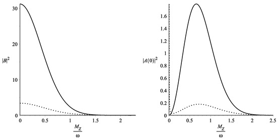
Figure 1.
as a function of parameter . Solid line is for , while the point line is for . as a function of parameter . Solid line is for , while the point line is for .
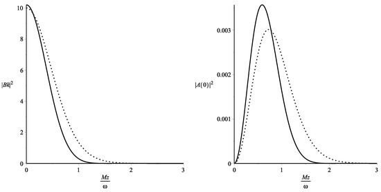
Figure 2.
as a function of parameter . Solid line is for , while the dotted line is for . as a function of parameter . Solid line is for , while the dotted line is for .
Figure 1 and Figure 2 show the variation of the probability density with the parameter and prove that the process of Z boson emission is important when the Hubble parameter is larger than the mass of the boson. Another consequence of the graphs is that the probability is finite and non-vanishing for and also for or . The ratio used in our graphs must be understood as and we observe that the probability is non-vanishing as long as the energy of the background is larger or has the same order as the rest of the energy of the Z boson. This result corresponds to the well-established knowledge that places the Z bosons production in the early universe. Our graphical results for the probability prove that in the Minkowski limit , the probabilities are vanishing, and this result can also be obtained by taking the limit in Equations (12) and (13). We can conclude that the process of Z boson emission by a neutrino is possible as a perturbative process only in early universe when the expansion factor is much larger than the Z boson mass.
3. Total Probability
In this section, we will analyze the situation when the expansion parameter is much larger than the Z boson mass. We will analyze the case of transversal polarization with . This can be achieved by observing that in Equation (8), the algebraic argument of the Bessel K functions become very small when , and we can use the following formula [24]:
where the real part of the index must meet the condition . In order to study the case where the expansion parameter is larger than the mass of the Z boson, we will consider the situation where . We mention that both the probabilities and amplitudes have a good behaviour in terms of parameter of the (see Figure 1 and Figure 2). We compute the total probability of transition in the case of large expansion, when and the index of Bessel K functions becomes . The total probability is obtained by solving the integrals after the final momenta. These kinds of integrals are in general divergent, and we will apply a method for regularization.
First, we obtain the transition amplitude in the limit by using Equations (8) and (11):
Then, the total probability expression of Z boson emission by a neutrino in the limit of large expansion is
To facilitate our calculations, we need to consider the case where the particles’ momenta are in the same direction, that is the z-axis, in such a way that the angle between the momenta vectors is 0, i.e., . In this case, the bispinor summation is reduced to a number. The momentum of the Z boson is also considered on the third axis such that . Then, the momenta integrals in total probability expression are
where we perform the delta Dirac integration, and finally we obtain an integral that is logarithmically divergent. To obtain a finite result, we will apply the dimensional regularization proposed in [25,26,27]. Then, we will replace our integral with a D-dimensional momenta integral as follows:
The new variable is introduced to obtain the integral of the Beta Euler function [24], as given in Appendix B, and the final result is
Because the result is still divergent for , we will use the relation between gamma Euler functions to obtain , which allows us to rewrite as
We observe that the above function is divergent in , and to remove the divergence, we use the method of minimal subtraction proposed in [27]. The pole of in has the following residue:
The method of minimal subtraction allows one to choose a counter-term dependent on a mass parameter with the general form , where s is taken such that the dimension of remains the same. Then, the renormalized integral is
The parenthesis from the above equation can be expanded around , and the result is
where is the digamma Euler function. Using this method, we successfully cancel the divergent term , and the final result of the renormalized integral is finite:
The final expression for the total probability for the process of Z boson emission by a neutrino in the early universe depends on the fundamental constants of the electro-weak theory
where in the second equality, we introduce the Fermi constant , i.e., , with representing the mass of the W boson.
4. The Rate of Transition
In the previous section, we computed the total probability for the process of Z boson emission by a neutrino in de Sitter geometry, but a fundamental problem is related to the computation of measurable quantities for such a process. For that, we will compute the rate of transition in this geometry, following the results obtained in [28] for the Milne universe. Consider the transition amplitude between the initial and final state in a de Sitter space–time of the form:
where the delta functions assure the momentum conservation in the process. In Equation (28), the usual delta function of energy is missing in de Sitter amplitudes. This problem comes from the temporal integrals denoted by :
whose results do not give the usual as in Minkowski space–time but instead have a rather complex dependence on hypergeometric Gauss functions as in Equations (6)–(8). The rate of transition is defined in Minkowski space–time by using the fact that the four delta Dirac functions when squared give the usual , where V is the volume and T is the interaction time. Then, the rate is obtained dividing the probability by , or in other words, the rate is the probability derivative with respect to time. Since in de Sitter geometry this is no longer valid, we adopt the definition given in [28], where the derivative with respect to time is applied on the integrals . These integrals are written in terms of conformal time , and the transition rate will be defined in conformal chart where we expect that the results are similar to those from the following Minkowski metric:
The above result for the rate of transition can be written now as shown below:
where represents the integrands from the temporal integrals given in Equations (8). Since in the present paper, the transition between states in a continuum spectrum are discussed, then to obtain the rate, we must integrate after the final momenta in Equation (31). Then, the rate definition for the process of Z emission by a neutrino is
where are the temporal integrals given in Equation (8) with the results given in Equations (10) and (11). The quantity is proportional to the coupling constants and the polarization terms . The function represents the integrands from Equation (8). All these quantities depend on . Knowing that the neutrino polarizations are fixed , we need to sum only after the Z boson polarizations .
The transition rate can be evaluated in the limit where the expansion parameter is larger than the mass of the Z boson by using the amplitude equation in this limit:
In the present case of large expansion, has the following expression:
while is given by
The limit from Equation (31) can be obtained by using the integrand in Equation (34):
Putting all the above quantities together and summing after the polarization, we obtain the transition rate:
which can be simplified by choosing the momenta of particles in the same direction:
The total transition rate is obtained by integration after the final momenta:
The momenta integral that needs to be computed is shown below:
In this case, we also use the dimensional regularization [25,26,27], and the D-dimensional integral reads
where the last equality in the above equation is obtained by making the variable change . The final result of the integral is obtained by using the definition of the Beta Euler function as shown:
which is divergent for . To remove the divergence, we apply the method of minimal subtraction [27]. First, we rewrite the divergent gamma function as
Then, becomes
The residue in is then computed
Then, the regularized integral is obtained by choosing a counter-term with the same dimension [27]
where is a bosonic mass parameter. The parenthesis expansion around then gives the following:
In this way, one can obtain the regularized result for the momenta integral:
The total transition rate is then given by a finite expression:
In Equation (49), we can obtain a numerical estimation for the transition rate of a Z boson emission by neutrino. Furthermore, one can establish the density number of Z bosons by taking into account the density numbers of neutrinos at different temperatures. For a very large number of neutrinos, this process could have an important impact to the Z boson generation, as we will discuss in the following section.
5. Density Number of Z Bosons
In the process of Z boson emission by neutrinos, the density number of neutrinos will determine the density number of Z bosons. For this reason, we define the density number of Z bosons with our transition rate given in Equation (49), as follows:
where is the rate of Z boson decay and is the density number of neutrinos in the conditions of early universe with the observation that all three species will be taken into account. It is a well-established fact that the Z bosons decay into fermion–anti-fermion pairs and hadrons. The total rate of the decay for the Z boson is the sum of the mentioned rates, and in Minkowski field theory, its value is GeV [29]. For the very early universe, the temperatures of photons and neutrinos are supposed to be equal such that the relations between the number of photons and neutrinos is [30]
where the primed values describe the density numbers in the early universe. From Equation (51), it is clear that the density number of neutrinos in the early universe will be higher, and we can say that the universe was dominated by neutrinos. As the temperature decreases and the universe expands, the neutrinos decouple and the number of neutrinos remains constant. This situation happens at temperatures around K. Now, let us comment on the implications in relation with our rate given in Equation (49).
Using the equations for the decay rate of Z bosons (49) and the number of neutrinos (51), the final equation for the density number of Z bosons produced in emission processes by neutrinos is
Taking into account the results given in Equations (51), we can obtain the density number of Z bosons per cubic centimeter produced in emission processes by neutrinos. For example, we set the temperature at K. The density number of neutrinos given in Equation (51) is . Then, the density number of Z bosons per cubic centimeter obtained from Equation (52) is
where we take the ration from the logarithm to be equal approximately to one. This result shows that in each cubic centimeter, we have around Z bosons, when the temperature was K. Using Equation (52), one can obtain the number densities of Z bosons at different temperatures with the observation that for a realistic evaluation, we need to keep the values around the temperatures specific to the end of the electro-weak epoch and hadron epoch when the Z bosons become massive [31]. Another observation is related to the fact that in our estimation, we use the decay rate from Minkowski theory. This result can be improved by using the decay rates in de Sitter space–time that also need to be evaluated in the limit of a large expansion factor.
At earlier times and high temperatures, it is also possible to study the number of Z bosons with the observation that the mass of the Z boson could be smaller or close to zero in these conditions, because the mass is related to the expectation values of the Higgs field. Another important step for a better understanding of our results is related to the establishing of the variation of the Z boson mass with the temperature via the expansion parameter, or the dependence on the form , where is the Hubble constant. This is an important issue that we hope to analyze in future research.
If the finite temperatures are considered, then the forbidden processes from Minkowski theory are allowed because of the energy received from the thermic bath, and this could be seen as similar to a certain degree to what the gravitational field can do on de Sitter space–time. This means that in the early universe, the thermic effect and the expansion effect could compete as mechanisms that generate particle production. For this reason, it is important to study both effects for a complete picture related to the problem of matter–antimatter generation in the early universe.
6. Conclusions
In this paper, we investigate the problem of particle production in the early universe by using a perturbative method that accounts for the generation of particles through fields’ interactions. Our results prove that for a clear picture of the mechanisms that were involved in matter production in the early universe, one should take into account the perturbative mechanism based on computations of the first-order transition amplitudes that have non-vanishing contributions in a non-stationary geometry. The mechanism proposed here could be one of the possible explanations for the abundance of Z bosons in the conditions of the early universe. We must point out that the rate computed in our paper is valid in the conformal chart , and the result was obtained by using the modes for the Dirac field and Proca field, which are defined globally in de Sitter manifold. Thus, we do not obtain the rate dependence on the observer, since this will imply the using of different modes in different charts and the Bogoliubov transformations. However, the perturbative result for the rate should be considered along with the cosmological results for a complete picture regarding the problem of particle production in the early universe, as was proved in [19]. To the best of our knowledge, the problem of cosmological production of massive bosons is less studied in the literature, and we hope that our perturbative results will be the start of the study of the Bogoliubov transformations in the case of the Proca field, which should also give the non-perturbative density number of massive bosons. One of the notable results related to the production of massive vector bosons in the FRLW universe was obtained in [32], where the density number was obtained using the Bogoliubov transformations. For further studies, it will be interesting to establish the behavior of the transition rate (32) and density number (52) at isometry transformations on de Sitter space–time. This should establish the invariance of this quantities in de Sitter geometry.
Our process is possible only in the early universe conditions where the expansion parameter is much larger than the Z boson mass, and this confirms the important results obtained in [19,33,34,35]. In these papers, the authors prove that the processes that involve particle production are possible only in early stages of the universe. Moreover, in [19], a perturbative method is used, and the results prove that the perturbative mechanism of particle production could become dominant in certain conditions. The results obtained in the present paper are in agreement with the important results mentioned above, and in addition is the first result from the literature that proposes the production of a Z boson in emission processes by neutrinos.
For a more complete result, all the perturbative processes that produce massive Z bosons must be studied in de Sitter space–time. The next step in this direction would be the study of the transition rates for the decays of the Z bosons into fermions in de Sitter geometry and their Minkowski limits, which are finite. Then, the total number of Z bosons could be in principle obtained for each process as the ratio between the production rates and the decay rates. Our present results also prove that the density number of Z bosons depends on temperatures that are specific to the end of the electro-weak epoch when the bosons become massive. In the Minkowski limit, when the expansion parameter is zero, the transition probabilities and rates are vanishing, and we recover the well-known result that the spontaneous Z boson generation by a neutrino in flat space–time is not allowed by the conservation of momentum and energy. Our results prove that in the conditions of the early universe, the Z bosons could be produced directly in spontaneous emission from vacuum with two fermions [2] or in emission processes by fermions, as we prove in the present study. These massive bosons could exist as stable particles in the early universe as long as the background energy was bigger or to the order of their rest energy, and these conditions are no longer met for the present-day expansion.
Author Contributions
Conceptualization, M.-A.B. and C.C.; Methodology, M.-A.B.; Software, C.C. and D.D.; Formal analysis, M.-A.B., C.C. and D.D.; Investigation, M.-A.B., C.C. and D.D.; Writing—original draft, C.C.; Writing—review & editing, M.-A.B. and D.D. All authors have read and agreed to the published version of the manuscript.
Funding
This work was supported by a grant of the Romanian Ministry of Research and Innovation and West University of Timişoara, CCCDI-UEFISCDI, under project “VESS, 18PCCDI/2018”, within PNCDI III.
Data Availability Statement
The data is available upon request from the authors.
Acknowledgments
We would like to thank Victor Ambrus for suggestions to improve the manuscript.
Conflicts of Interest
The authors declare no conflict of interest.
Appendix A. Free Fields in de Sitter Geometry
In Equation (2), the solutions of the Dirac equations for zero mass field are used. These solutions describe the neutrino field in de Sitter geometry, and their explicit form was obtained in [20]
The form of the helicity bispinors can be expressed as follows [15]:
while . These spinors satisfy the following relation:
with , where are the Pauli matrices and is the modulus of the momentum vector. In the case of a Proca field, the temporal and spatial solutions in de Sitter geometry are obtained in [21]. The spatial part of the solution is given by
while the temporal part of the solution of the Proca equation [21] is given by:
In the solutions for the Proca equation on a momentum basis, the polarization vectors are and . For , the polarization vectors are transversal, . In the case , the polarization vectors are longitudinal on the momentum , since . The notation for the mass of the Z boson is , and the parameter is dependent on the ratio , and the condition assures that the index of the Hankel function is imaginary.
Appendix B. Integrals for Obtaining the Amplitude and Rate
The temporal integrals from amplitude are of the following type [24]:
The integral of the Beta Euler function is given by
and in our case, the values for arguments are .
References
- Crucean, C. Production of Z bosons and neutrinos in early universe. Eur. Phys. J. C 2019, 79, 483. [Google Scholar] [CrossRef]
- Dumitrele, D.; Băloi, M.A.; Crucean, C. A perturbative production of massive Z bosons and fermion–antifermion pairs from the vacuum in the de Sitter Universe. Eur. Phys. J. C 2023, 83, 738. [Google Scholar] [CrossRef]
- Crucean, C.; Fodor, A.D. Production of massive W ± bosons and fermion–antifermion pairs from vacuum in the de Sitter Universe. Eur. Phys. J. C 2023, 83, 929. [Google Scholar] [CrossRef]
- Weinberg, S. A Model of Leptons. Phys. Rev. Lett. 1967, 19, 1264. [Google Scholar] [CrossRef]
- Weinberg, S. Physical Processes in a Convergent Theory of the Weak and Electromagnetic Interactions. Phys. Rev. Lett. 1971, 27, 1688. [Google Scholar] [CrossRef]
- Weinberg, S. Effects of a Neutral Intermediate Boson in Semileptonic Processes. Phys. Rev. D 1972, 5, 1412. [Google Scholar] [CrossRef]
- Weinberg, S. General Theory of Broken Local Symmetries. Phys. Rev. D 1973, 7, 1068. [Google Scholar] [CrossRef]
- Weinberg, S. Current Algebra and Gauge Theories. I. Phys. Rev. D 1973, 8, 605. [Google Scholar] [CrossRef]
- Weinberg, S. Recent progress in gauge theories of the weak, electromagnetic and strong interactions. Rev. Mod. Phys. 1974, 46, 255. [Google Scholar] [CrossRef]
- Weinberg, S. Beyond the First Three Minutes. Phys. Scr. 1979, 21, 773. [Google Scholar] [CrossRef]
- Glasshow, S.L.; Weinberg, S. Natural conservation laws for neutral currents. Phys. Rev. D 1977, 15, 1958. [Google Scholar] [CrossRef]
- Bjorken, J.D.; Lane, K.; Weinberg, S. Decay μ→ e γ in models with neutral heavy leptons. Phys. Rev. D 1977, 5, 1474. [Google Scholar] [CrossRef]
- Lee, B.W.; Weinberg, S. SU(3)⨂U(1) Gauge Theory of the Weak and Electromagnetic Interactions. Phys. Rev. D 1977, 38, 1237. [Google Scholar]
- Rubbia, C. Experimental observation of the intermediate vector bosons W+, W-, and Z 0. Rev. Mod. Phys. 1985, 57, 699. [Google Scholar] [CrossRef]
- Weinberg, S. The Quantum Theory of Fields; Cambridge University Press: Cambridge, UK, 1995. [Google Scholar]
- Cosmin, C. Fermion production in a Coulomb field on a de Sitter universe. Phys. Rev. D 2012, 85, 084036. [Google Scholar] [CrossRef]
- Crucean, C.; Băloi, M.A. Fermion production in a magnetic field in a de Sitter universe. Phys. Rev. D 2016, 93, 044070. [Google Scholar] [CrossRef]
- Cotăescu, I.I.; Crucean, C. de Sitter QED in Coulomb gauge: First order transition amplitudes. Phys. Rev. D 2013, 87, 044016. [Google Scholar] [CrossRef]
- Birrel, N.D.; Davies, P.C.W.; Ford, L.H. Effects of field interactions upon particle creation in Robertson-Walker universes. J. Phys. A 1980, 13, 961. [Google Scholar] [CrossRef]
- Cotăescu, I.I. Polarized Dirac fermions in de Sitter spacetime. Phys. Rev. D 2002, 65, 084008. [Google Scholar] [CrossRef]
- Cotăescu, I.I. Polarized vector bosons on the de Sitter expanding universe. Gen. Rel. Grav. 2010, 42, 861–876. [Google Scholar] [CrossRef]
- Misner, C.W.; Thorne, K.S.; Wheleer, J.A. Gravitation; W. H. Freeman and Company: New York, NY, USA, 1973. [Google Scholar]
- Weinberg, S. Cosmology; Oxford University Press: Oxford, UK, 2008. [Google Scholar]
- Gradshteyn, I.S.; Ryzhik, I.M. Table of Integrals, Series and Products; Academic Press: Cambridge, MA, USA, 2007. [Google Scholar]
- Hooft, G.; Veltman, M. Regularization and renormalization of gauge fields. Nucl. Phys. B 1972, 44, 189. [Google Scholar]
- Bollini, C.G.; Giambiagi, J.J. Dimensional renorinalization: The number of dimensions as a regularizing parameter. Nuovo Cimento B 1972, 12, 20. [Google Scholar] [CrossRef]
- Hooft, G. Dimensional regularization and the renormalization group. Nucl. Phys. B 1973, 61, 455. [Google Scholar] [CrossRef]
- Cotăescu, I.I.; Popescu, D. First order QED processes in a spatially flat FLRW space-time with a Milne-type scale factor. Chin. Phys. C 2020, 44, 055104. [Google Scholar] [CrossRef]
- Tanabashi, M.; Particle Data Group. 2018 Review of Particle Physics-29. Cosmic rays. Phys. Rev. D 2018, 98, 030001. [Google Scholar] [CrossRef]
- Steigman, G. Massive relic neutrinos—A status report. Nucl. Phys. B 1985, 252, 73. [Google Scholar] [CrossRef]
- Fritzsch, H. Fundamental constants at high energy. Fortschr. Phys. 2002, 50, 518. [Google Scholar] [CrossRef][Green Version]
- Ema, Y.; Nakayama, K.; Tang, Y. Production of purely gravitational dark matter: The case of fermion and vector boson. J. High Energy Phys. 2019, 2019, 60. [Google Scholar] [CrossRef]
- Schrödinger, E. The proper vibrations of the expanding universe. Physica 1939, 6, 899. [Google Scholar] [CrossRef]
- Parker, L. Particle creation in expanding universes. Phys. Rev. Lett. 1968, 21, 562. [Google Scholar] [CrossRef]
- Parker, L. Quantized fields and particle creation in expanding universes. I. Phys. Rev. 1969, 183, 1057. [Google Scholar] [CrossRef]
Disclaimer/Publisher’s Note: The statements, opinions and data contained in all publications are solely those of the individual author(s) and contributor(s) and not of MDPI and/or the editor(s). MDPI and/or the editor(s) disclaim responsibility for any injury to people or property resulting from any ideas, methods, instructions or products referred to in the content. |
© 2024 by the authors. Licensee MDPI, Basel, Switzerland. This article is an open access article distributed under the terms and conditions of the Creative Commons Attribution (CC BY) license (https://creativecommons.org/licenses/by/4.0/).