Meson Condensation

Abstract

We give a pedagogical review of the properties of the various meson condensation phases triggered by a large isospin or strangeness imbalance. We argue that these phases are extremely interesting and powerful playground for exploring the properties of hadronic matter. The reason is that they are realized in a regime in which various theoretical methods overlap with increasingly precise numerical lattice QCD simulations, providing insight on the properties of color confinement and of chiral symmetry breaking.

1. Introduction

The great success of the Standard Model of particle physics relies on the possibility of making accurate and testable predictions that are in agreement with increasingly precise experimental data. Despite this success, many aspects of the Standard Model are still not completely clear. Among these, there are the mechanisms of color confinement and of chiral symmetry breaking ($\chi$SB) of the strong interaction. The typical energy scales of confinement and $\chi$SB pertain to the nonperturbative region of quantum chromodynamics (QCD), which makes their study extremely challenging.

For some theoreticians, the confinement and the $\chi$SB mechanisms are uninteresting because they are details of a robust theoretical construction, thus sooner or later they will be fully understood; for others (including the author), unraveling the origin of these mechanisms is of the utmost importance for a comprehensive understanding of QCD; for all, it is still unclear which is the path that can bring us to a full understanding of these mechanisms. My view is that any path, as far it is physically sound, should be explored and tested. This brief review is about one those paths, exploring the behavior of matter when there is an asymmetry in the number of particles with different isospin and/or strangeness. This seems a promising direction because a number of theoretical methods can be used for studying these phases. Comparing the results obtained by different methods helps us to check their consistency and the degree of the reached accuracy.

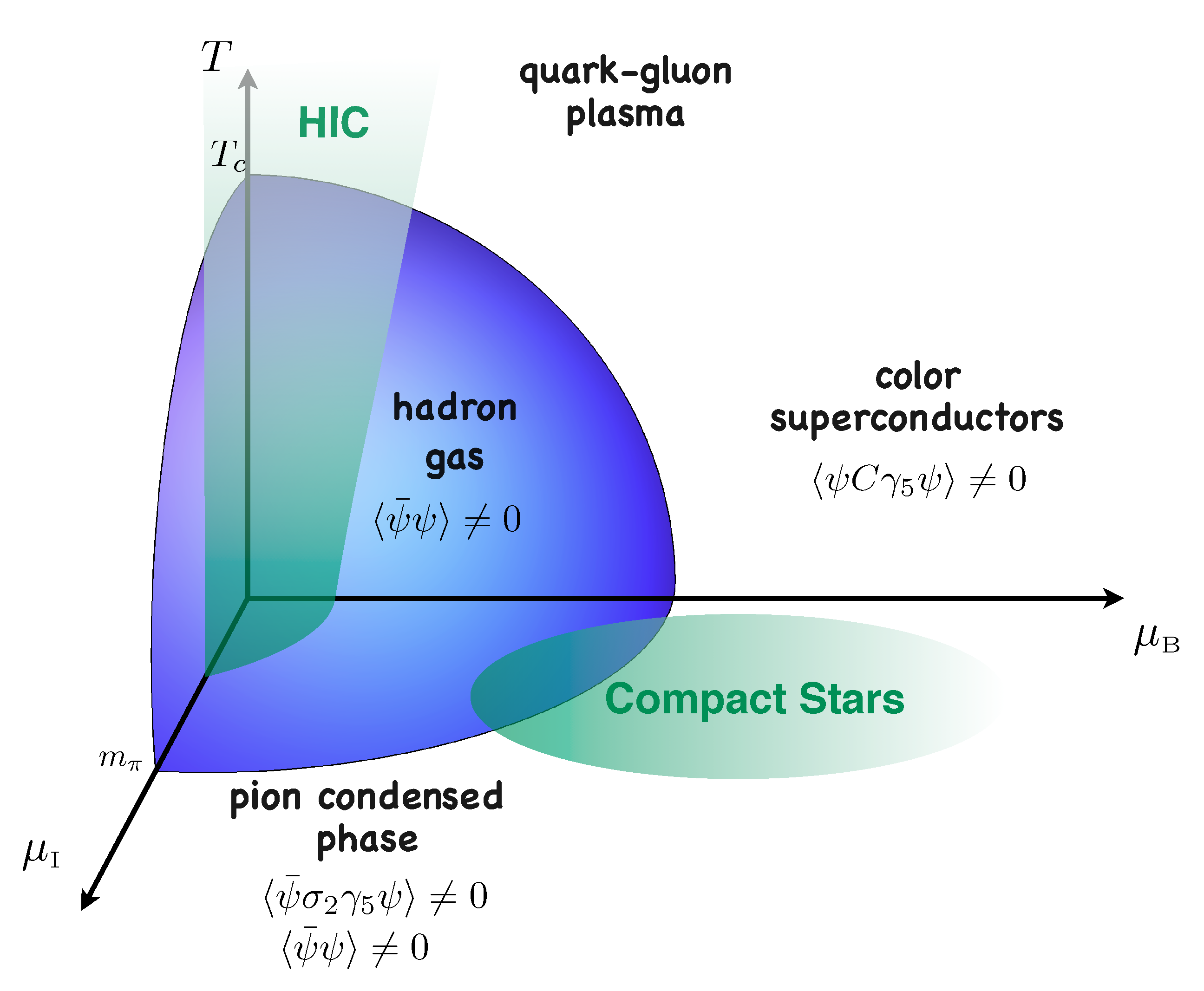
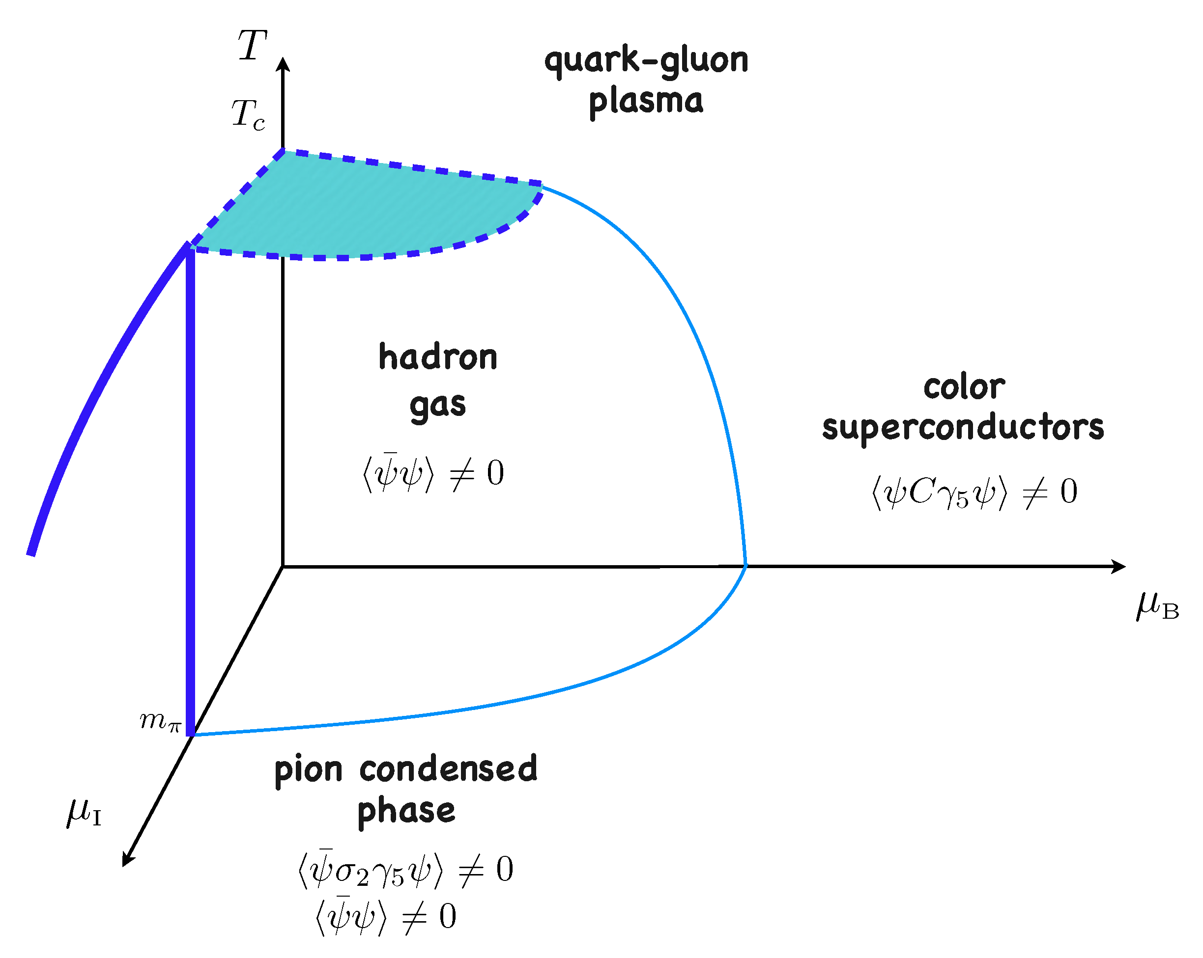
To clarify the setting we report in Figure 1 a sketch of the so-called QCD phase diagram: a grand canonical description of the phases of hadronic matter as a function of the hadronic temperature, T, of the isospin chemical potential, ${\mu }_I$, and of the baryonic chemical potentials, ${\mu }_B$. The total baryonic density is determined by ${\mu }_B$, while ${\mu }_I$ describes the isospin asymmetry, say due to a different number of up and down quarks. If it were possible we would have added a further axis, ${\mu }_S$, indicating the strangeness content. The blue region corresponds to a gas of confined hadrons with a chiral broken symmetry. At large energy scales quarks and gluons should be liberated [1] realizing different phases. We have indicated three of them. The quark-gluon plasma (QGP), realized at large temperature, is asymptotically a gas of quarks and gluons that becomes strongly interacting for the temperature reachable in heavy-ion collisions, see for instance [2,3,4]. At large ${\mu }_B$ we expect that deconfined quarks fill their Fermi spheres and that the color interaction drives the formation of Cooper pairs in a BCS-like color superconducting phase (CSC), see [5,6,7] for reviews. At large and positive ${\mu }_I$ we expect to populate the u and $\overline{d}$ states with the color interaction inducing the formation of ${\pi }^{+}$ states that will eventually condense. A negative isospin chemical potential does instead favor the formation of ${\pi }^{-}$ states. Whether these phases persist to the hadron gas surface of Figure 1 depends on the non-perturbative properties of QCD. This diagram is somehow our starting point to set the stage, we will review it in Section 5 feeding in the up to date results. For the time being we note that there are two uncontroversial results: The critical temperature $T_c\sim 160$ MeV has been experimentally investigated at RHIC and at LHC and precisely determined by LQCD simulations [8,9] to correspond to a analytic crossover. The transition to the pion condensed phase at $T=0$ is a second order phase transition happening exactly at ${\mu }_I=m_{\pi }$ [10,11].

Outside the Beta-Equilibrated Sheet

The three chemical potentials, ${\mu }_B,{\mu }_I$ and ${\mu }_S$ are not three independent quantities because the weak interactions regulate the isospin and strangeness content of matter at a given baryonic density. Moreover, matter must be electrically neutral and the strong interactions can modify the dispersion laws of quasiparticles. Therefore, we should indicate in Figure 1 a beta-equilibrated sheet ${\mu }_I=f({\mu }_B,T)$, where f is some equation of state giving the isospin asymmetry at any temperature and baryonic chemical potential. The beta-equilibrated sheet corresponds to the configuration realized in long lived systems, as in compact stars. It is however instructive to consider configurations outside this surface, for three main reasons. The first is that we do not actually know f, except in restricted energy regions: at small energy scales by nuclear experiments, and at asymptotically large energy scales by perturbative QCD; the second is that in the theoretical investigation we can turn off the weak interactions, thus we can compare the outcomes of different theoretical methods outside the beta-equilibrated sheet to test their robustness and consistency. Finally, working on the beta-equilibrated sheet is interesting for studying the properties of dense nuclear matter in compact stars, but makes the problem so complicated that it is presently hard to make predictions.

In the first papers discussing the pion condensation [12,13], Migdal tried to work on the beta-equilibrated sheet considering how nuclear matter mechanisms could make the ${\pi }^0$ stable states. Then, different authors [14,15,16] considered the possible mechanisms for in-medium stabilization of charged pions by a softening of the pion spectrum by the p-wave pion-nucleus interaction. The in-medium pion dispersion law was assumed to be

$${\omega }^2\left(k\right)=m_{\pi }^2+0.7n{m}_{\pi }\omega +k^2(1-6n),$$

(1)

where n is the baryonic density in units of fm${}^{-3}$. The exciting result is that a gapless mode appears for $n>1/6$ fm${}^{-3}$, thus very close to the nuclear saturation density $n_0\sim 0.16$ fm${}^{-3}$, at a momentum $k=m_{\pi }/\sqrt{6n-1}$. Therefore, a transition to a superfluid phase was expected just above the nuclear saturation density. However, it was pointed out by Migdal [17] that the $\pi -\pi$ repulsive interaction may qualitatively change this result and he argued in favor of ${\pi }^0$ condensation as well as stable ${\pi }^{+}{\pi }^{-}$ molecules. Still today we have not solved this problem, but most of the theoretical works are now directed to understanding what happens outside the beta-equilibrated sheet. This new approach has allowed Son and Stephanov [10] to qualitatively and quantitatively assess the main properties of the pion condensed phase by the use of a simple approach based on the modelization of QCD by chiral perturbation theory ($\chi$PT) [10,11].

Actually, there is a number of theoretical approaches that can be used. In principle, any information on the phase diagram of Figure 1 could be obtained introducing in the QCD action a chemical potential for the charge of interest. The QCD Lagrangian turns to be

$${\mathcal{L}}_{\mathrm{QCD}}=\overline{\psi }\left[{\gamma }^{\mu }\left(i{D}_{\mu }\right)-M\right]\psi -\frac{1}{4}{F}_{\mu \nu }^a{F}^{a,\mu \nu },$$

(2)

where $F_{\mu \nu }^a$ with $a=1,\dots ,8$ are the color gauge field strengths, ${\psi }^T=(u,d,s)$ is the spinor describing up, down and strange quarks (with suppressed color and spinorial indices), the bare quark masses are collected in the mass matrix

$$M=\mathrm{diag}(m,m,m_s),$$

(3)

where we have assumed degenerate light quark masses, and the covariant derivative

$$D_{\mu }={\partial }_{\mu }+ig{A}_{\mu }-\frac{i}{2}{v}_{\mu },$$

(4)

includes both the minimal interaction with the gauge fields, $A_{\mu }$, and with the external source

$$v_{\mu }=2\mu {\delta }_{\mu 0},$$

(5)

with the chemical potentials collected in the matrix

$$\mu =\mathrm{diag}\left({\mu }_u,{\mu }_d,{\mu }_s\right)=\frac{{\mu }_B-{\mu }_S}{3}\mathcal{I}+{\mu }_I{T}_3+\frac{2{\mu }_S}{\sqrt{3}}{T}_8,$$

(6)

where $T_3$ and $T_8$ are the two diagonal $SU\left(3\right)$ generators, $\mathcal{I}$ is the $3\times 3$ identity matrix and we have parameterized the quark chemical potentials as ${\mu }_{u,d}={\mu }_B/3\pm {\mu }_I/2$ and ${\mu }_s={\mu }_B/3-{\mu }_S$. To determine the phase diagram in Figure 1 one should obtain the behavior of the chiral, pion and diquark condensates, respectively given by

$$\begin{array}{cc}\hfill \sigma & \propto \langle \overline{\psi }\psi \rangle ,\hfill \end{array}$$

(7)

$$\begin{array}{cc}\hfill {\pi }_a& \propto \langle \overline{\psi }{\sigma }_a{\gamma }_5\psi \rangle ,\hfill \end{array}$$

(8)

$$\begin{array}{cc}\hfill \Delta & \propto \langle \psi C{\gamma }_5\psi \rangle ,\hfill \end{array}$$

(9)

where ${\sigma }_a$ with $a=1,2,3$ are the Pauli matrices, as a function of T, ${\mu }_B$ and ${\mu }_I$.

Given the nonperturbative character of QCD at the energy scales of the various phase transitions in Figure 1, the Lagrangian in Equation (2) is of little direct use. Various theoretical approaches have been developed, including linear sigma models and chiral perturbation theory ($\chi$PT) [10,11,18,19,20,21,22,23,24,25,26,27,28,29,30,31,32,33], the Nambu-Jona Lasinio (NJL) models [34,35,36,37,38,39,40,41,42,43,44,45,46,47,48,49,50,51,52,53,54,55,56], the quark-meson models [57,58,59,60,61,62], the random matrix model [63,64], the AdS/QCD model [65] and perturbative QCD (pQCD) (with diagrams resummation) [66,67]. A guiding role in this forest of theoretical approaches is played by the lattice QCD (LQCD) simulations [68,69,70,71,72,73,74,75,76,77,78,79,80,81,82], which provide a powerful tool for a numerical check and for exploring non-perturbative QCD. As we shall discuss in some detail in Section 4.3, the grand-canonical LQCD simulations at finite baryonic density and/or strangeness density are hampered by the so-called sign problem, but are feasible at ${\mu }_B={\mu }_S=0$ and ${\mu }_I\ne 0$ [68]; moreover it is possible to simulate an ensemble of kaons by the canonical LQCD approach [74,75], corresponding to a system at nonvanishing strangeness density, as discussed in more detail in Section 4.3. This places the study of the meson condensation on a firmer ground with respect to the study of the phases at large baryonic density: the various theoretical models (we will mostly focus on $\chi$PT and the NJL model) give a qualitative and semiquantitative description of the meson condensed phase; the LQCD simulations provide numerical evidence for the proposed phase transitions and for the meson properties. The theoretical understanding at large ${\mu }_B$ cannot count on experimental data nor on numerical simulations. The phases realized at high baryonic densities could be relevant for dense stellar objects, but it is hard to obtain constraints on the microscopic properties of matter from the macroscopic properties of compact stars [83,84].

This review is organized as follows. In Section 2 we investigate the stability of pions in nuclear matter by a simplified non-interacting model description of hadronic matter. This model, mainly used in the 1960s and in the 1970s, serves as a guide for understanding by simple qualitative reasoning how meson condensation can occur and why it is unclear whether it be realized in compact stars or any other stellar object. In Section 3 we use an argument based on group theory to derive the phase diagram of the meson condensed phases. This is a useful result because any other theoretical modeling is expected to reproduce this phase diagram. In Section 4 we report and compare the results obtained by three different approaches: $\chi$PT, NJL and LQCD, showing that the obtained results are in qualitative and quantitative agreement for $T=0$ and ${\mu }_I\lesssim 2m_{\pi }$. At nonvanishing temperature the three approaches give similar qualitative results, but more work is needed to reconcile the $\chi$PT and NJL methods with the precise numerical results of the LQCD simulations. We conclude, with a new discussion of the QCD phase diagram, in Section 5.

2. The Early Works and Models

To understand why the pion condensation in dense hadronic matter is controversial [85] we scrutinize the condition for the meson stabilization against weak decays by a simple non-interacting gas approximation (NGA). This is a mean field model based on the assumption that neutrons, protons and electrons behave as independent Fermi gases of quasiparticles. As we shall see below, the result of these kind of models is that fermions are favored with respect to mesons [86,87,88,89,90]. The pion states can only be populated at non extreme densities if the strong interaction modifies the pion spectrum.

2.1. The Equilibrium Configuration

The condensation mechanism of any type of particle relies on three basic requirements:

• The particles must be bosons, as ${}^4$He atoms, or boson-like, as Cooper pairs in the BCS theory
• The system has to be sufficiently cold: the particle condensation can be disrupted by the thermal disorder
• The particles must be stable.

Since mesons are bosons, they satisfy the first requirement. We can also imagine that they can be produced in a relatively cold environment, as in the core of neutron stars [83]. The third point is typically neglected in ultracold atom physics, because experiments are done with stable atoms [91]. In contrast, all mesons in vacuum are unstable. The point is whether medium effects can stabilize mesons or not.

The first papers discussing stable pions in dense nuclear matter appeared in the 1960s [86,87,88,89] considering a medium of catalyzed nuclear matter: neutral matter consisting of nucleons and leptons in electroweak equilibrium. In the Fermi gas approximation, the equilibrium distribution is determined by the Urca process

$$n\to p+e+{\overline{\nu }}_{e}p+e\to n+{\nu }_e,$$

(10)

that with the assumption of neutrino transparency implies that

$${\mu }_n={\mu }_p+{\mu }_e,$$

(11)

where ${\mu }_i$, with $i=n,p,e$, are the appropriate chemical potentials, see [92] for the temperature corrections to the Fermi gas approximation. The electrical neutrality requires that

$$n_p=n_e,$$

(12)

where $n_p$ and $n_e$ are the number densities of protons and electrons, respectively.

In the NGA, the number density of each component is

$$n_i=2{\int }_0^{p_{f,i}}\frac{d^{3}p}{{\left(2\pi \right)}^3}=\frac{p_{f,i}^3}{3{\pi }^2},$$

(13)

with $p_{f,i}$ the Fermi momentum. The neutrality condition Equation (12) then implies that the Fermi momenta of electrons and protons are the same, that is

$$p_{f,p}=p_{f,e}\simeq {\mu }_e,$$

(14)

where in the last expression we have neglected the electron mass. For free Fermi gases, without in-medium effects, we obtain using Equation (11) that

$$p_{f,n}\simeq 2{\mu }_e({\mu }_e+\sqrt{{\mu }_e^2+m_n^2}),$$

(15)

where $m_n$ is the nucleon mass (we have neglected the small mass difference between protons and neutrons). Upon substituting these expressions in Equation (13) we can express any number density as a function of the electron chemical potential; in particular, the total number density as an increasing function of the electron chemical potential. We can now include different hadronic states. We determine and compare, for reasons that will soon become clear, the threshold electron chemical potential for the appearance of ${\pi }^{-}$ and ${\Sigma }^{-}$.

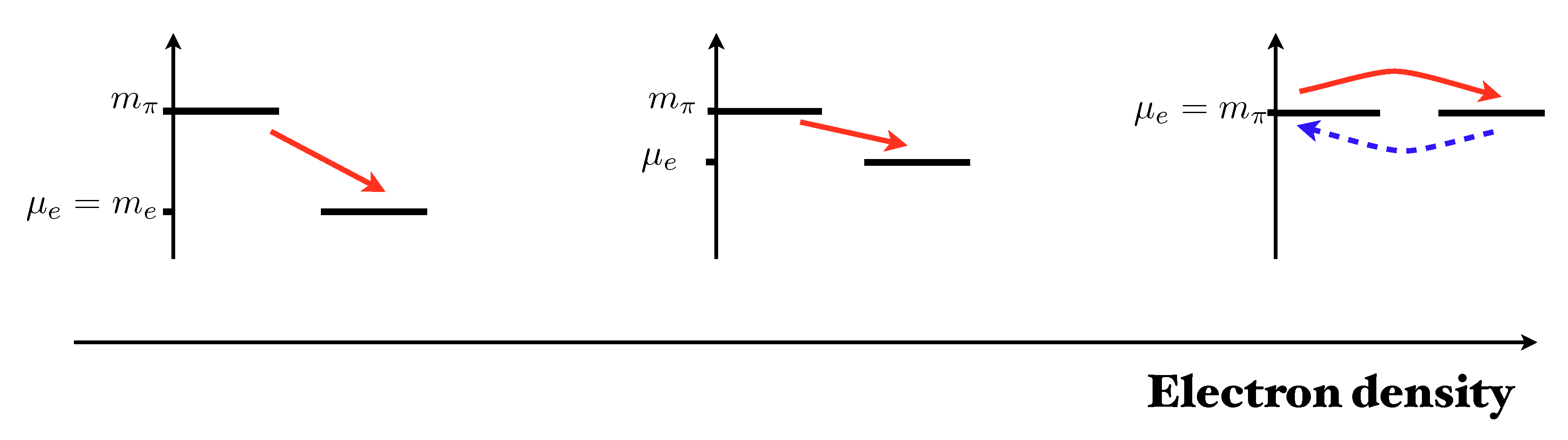
In vacuum ${\pi }^{-}$ decays to leptons, mostly in muon and in its antineutrino. Since muons decay in electrons and neutrinos, we simplify the discussion considering the process (solid red line in Figure 2)

$${\pi }^{-}\to e^{-}+{\overline{\nu }}_e,$$

(16)

where we assume that neutrinos are not trapped. This process can be Pauli blocked as depicted in the right side of Figure 2, meaning that it is in equilibrium with the electron decay process (dashed blue line in Figure 2)

$$e^{-}\to {\pi }^{-}+{\nu }_e,$$

(17)

in the configuration with

$${\mu }_{e\pi }=m_{\pi }\simeq 135\mathrm{MeV}.$$

(18)

We now proceed with a similar analysis for the stability of the ${\Sigma }^{-}$ baryonic resonance. In the quark model it is a $\left(dds\right)$ state with mass, $m_{{\Sigma }^{-}}\simeq 1.2$ GeV, weakly decaying by

$${\Sigma }^{-}\to n{\pi }^{-}\to n+e^{-}+{\overline{\nu }}_e,$$

(19)

in about ${10}^{-10}$ s. The ${\Sigma }^{-}$ states can be populated by the electron capture process

$$e^{-}+n\to {\Sigma }^{-}+{\nu }_e,$$

(20)

with eventually an additional spectator neutron to ensure the energy-momentum conservation. The equilibrium is reached at

$${\mu }_{e\Sigma }=\frac{2m_{{\Sigma }^{-}}-\sqrt{m_{{\Sigma }^{-}}^2+3m_p^2}}{3}\simeq 126\mathrm{MeV},$$

(21)

and since ${\mu }_{e\pi }>{\mu }_{e\Sigma }$ the ${\Sigma }^{-}$ states appear at a lower density than the ${\pi }^{-}$ states. This result is somehow surprising: at high density the heavier ${\Sigma }^{-}$ states are favored over the lighter mesonic ${\pi }^{-}$ states. This happens because the production channels of these two hadrons are different and because the ${\Sigma }^{-}$ is not much heavier than nucleons. The density for the appearance of the ${\Sigma }^{-}$ states in the NGA is pretty large, about $4n_0$. Once the ${\Sigma }^{-}$ states are populated they must be included in the neutrality condition in Equation (12), forbidding the appearance of pions up to $n\sim 300n_0$, see for instance [90] and references therein.

2.2. Including in-Medium Effects

Although in the free gas approximation the ${\pi }^{-}$ is not energetically favored with respect to ${\Sigma }^{-}$, the difference between the two critical chemical potentials is small, ${\mu }_{e\pi }-{\mu }_{e\Sigma }\simeq 10\mathrm{MeV}\ll m_{\pi }$. Thus, a slight change of their effective masses may invert this result: charged pion states could be populated first.

To gain insight, we assume that the the strong interactions cause a constant Fermi energy shift [90], independent of the particle momentum. In the NGA framework, for any baryon i, we define the effective chemical potential

$${\mu }_{\mathrm{eff},i}={\mu }_i-{\overline{B}}_i,$$

(22)

where ${\overline{B}}_i$ is the constant chemical energy shift due to the strong interactions, while for leptons ${\overline{B}}_{\mathrm{lepton}}=0$. The chemical equilibrium, Equation (11), now reads

$${\mu }_{\mathrm{eff},n}={\mu }_{\mathrm{eff},p}+{\mu }_e,$$

(23)

where we have assumed as before that neutrinos escape: the medium does not trap neutrinos. Turning to the problem of populating ${\pi }^{-}$ and ${\Sigma }^{-}$ states, the charged pion states are now populated (do not decay in leptons) at

$${\mu }_{e\pi }=m_{\pi }-{\overline{B}}_{\pi },$$

(24)

thus a positive $B_{\pi }$ favors the appearance of ${\pi }^{-}$. The ${\Sigma }^{-}$ appears at the critical electron chemical potential in Equation (21) with

$$m_{{\Sigma }^{-}}\to m_{{\Sigma }^{-}}-{\overline{B}}_{{\Sigma }^{-}}+{\overline{B}}_p,$$

(25)

therefore assuming small binding energies we find that pions appear first (${\mu }_{e\pi }\le {\mu }_{e\Sigma }$) for

$${\overline{B}}_{\pi }-0.47({\overline{B}}_{{\Sigma }^{-}}-{\overline{B}}_p)\gtrsim 10\mathrm{MeV},$$

(26)

which is a condition depending on three in-medium quantities.

The point of this simple model is that the appearance of pions may or may not happen depending on quite small parameters that are not under quantitive control. In particular, it is not clear in which direction the medium effects go [90]. Any result obtained in this way can hardly stand firm against scrutiny and it is doomed to be troublesome, because based on a too naive modeling and/or on extrapolating nuclear matter properties at least to $2-3n_0$ [19].

3. Group Theory Analysis

In recent years a simpler approach to the mechanism of meson condensation has been developed, disentangling it from weak equilibrium and strong interaction effects. We illustrate it for pions. Pions are an isospin triplet: they are the three eigenstates of an $I=1$ multiplet with different $I_3$ projection. In vacuum the masses of the charged pions are degenerate, however this degeneracy is removed by the isospin chemical potential as in the Stark-Lo Surdo effect. In particular, we expect that the energy levels split as follows

$$\begin{array}{cc}\hfill E_{{\pi }^0}& =\sqrt{m_{\pi }^2+p^2},\hfill \end{array}$$

(27)

$$\begin{array}{cc}\hfill E_{{\pi }^{-}}& =+{\mu }_I+\sqrt{m_{\pi }^2+p^2},\hfill \end{array}$$

(28)

$$\begin{array}{cc}\hfill E_{{\pi }^{+}}& =-{\mu }_I+\sqrt{m_{\pi }^2+p^2},\hfill \end{array}$$

(29)

which are valid for $|{\mu }_I|<m_{\pi }$, because for $|{\mu }_I|>m_{\pi }$ one of the two charged mesons becomes massless. This is an indication of a spontaneous symmetry breaking (SSB), with the resulting massless mode to be identified with the Nambu-Goldstone boson (NGB) associated to a broken generator. The best tool for exploring the (global) symmetry breaking is group theory. The good thing about this method is that it gives robust results. Its main limitation is that it does not provide a microscopic mechanism for the occurrence of the symmetry breaking.

3.1. Global Symmetries of QCD

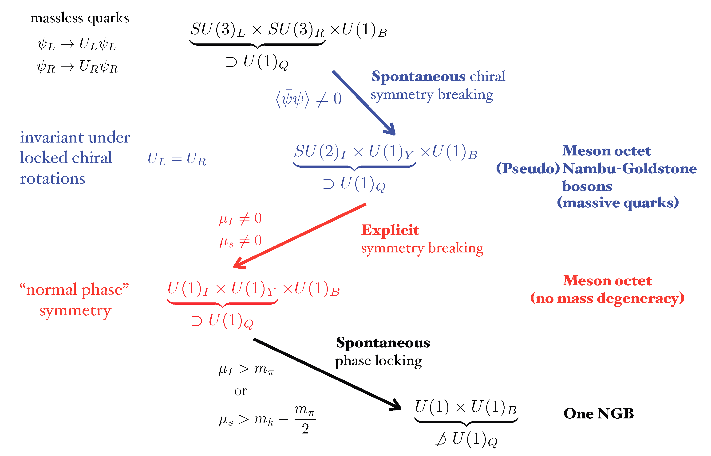
In Figure 3 we report the global symmetry breaking pattern which is relevant for meson condensation. We start assuming three flavor massless quarks with ${\mu }_I={\mu }_S=0$ described by an Hamiltonian, $\mathcal{H}$, with global symmetries

$$\mathrm{G}=\underset{{\displaystyle \supset U{\left(1\right)}_Q}}{\underbrace{SU{\left(3\right)}_L\times SU{\left(3\right)}_R}}\times U{\left(1\right)}_B,$$

(30)

where we have not included the $U{\left(1\right)}_A$ anomalous group and we have specified that the electromagnetic gauge group, $U{\left(1\right)}_Q$, is a subgroup of the considered symmetries. The baryon symmetry group, $U{\left(1\right)}_B$, can be broken by the formation of quark Cooper pairs in the CSC phase, see Figure 1. In the following we will not consider this possibility, focusing on the chiral symmetry, $SU{\left(3\right)}_L\times SU{\left(3\right)}_R$, corresponding to the invariance of massless QCD with respect to left- and right-handed rotations, indicated respectively with $U_L$ and $U_R$ in Figure 3, of the quark fields.

In vacuum the chiral condensate locks the chiral rotation to the vectorial flavor group by the SSB

$$\mathrm{G}\to \underset{{\displaystyle \supset U{\left(1\right)}_Q}}{\underbrace{SU{\left(3\right)}_V}}\times U{\left(1\right)}_B,$$

(31)

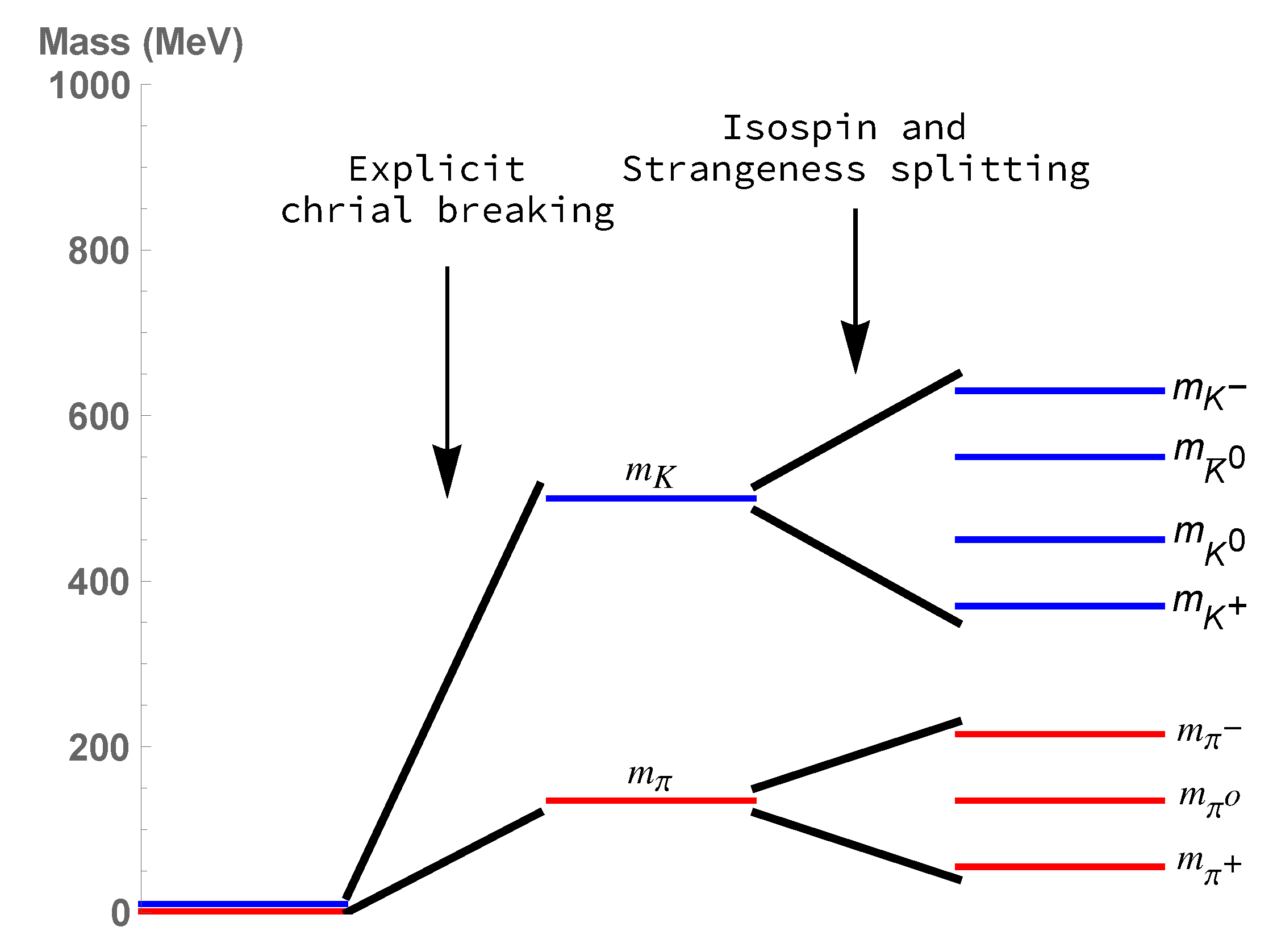
corresponding to the simultaneous rotations of left- and right-handed quark fields. The ground state is still invariant under rotation of quark flavors but the left and right handed rotations are now locked: the quark transformation leaving the vacuum invariant is $U_L=U_R$. According to the Goldstone’s theorem this symmetry breaking pattern results in 8 NGBs associated to the broken generators, see the left side of Figure 4. Actually, the bare quark masses explicitly break the chiral symmetry, meaning that these modes are massive pseudo NGBs, identified with the pseudoscalar meson octet. Assuming that the light quark masses are degenerate the isospin symmetry is preserved, meaning that the resulting symmetry is now (second row of Figure 3)

$$\underset{{\displaystyle \supset U{\left(1\right)}_Q}}{\underbrace{SU{\left(2\right)}_I\times U{\left(1\right)}_Y}}\times U{\left(1\right)}_B,$$

(32)

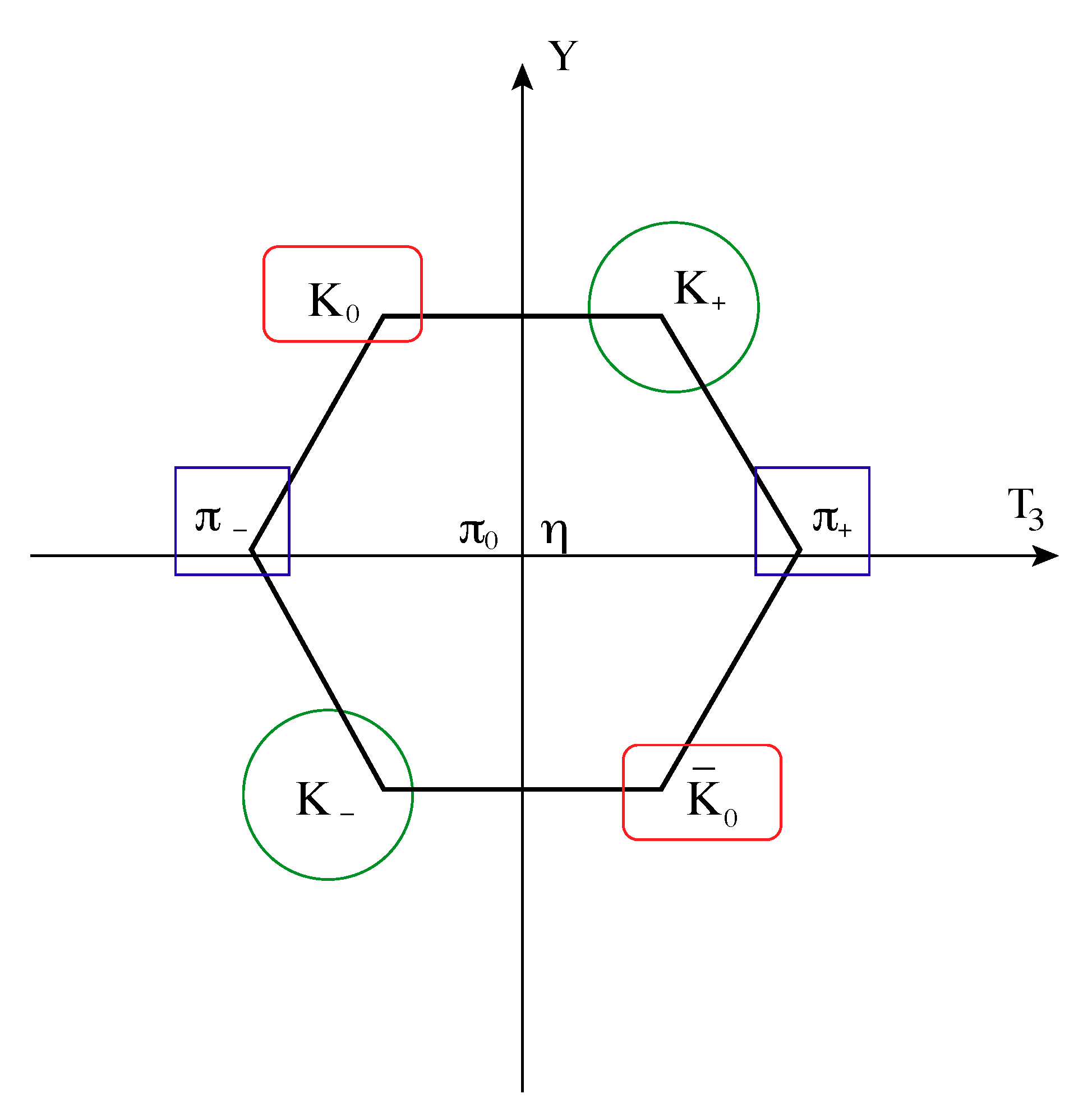
where $SU{\left(2\right)}_I$ is the isospin symmetry group and $U{\left(1\right)}_Y$ is the symmetry group generated by $T_8$. Thanks to the isospin invariance the pions are degenerate, with mass $m_{\pi }\simeq 135$ MeV. The kaons are grouped in two isodoublets with degenerate masses $m_K\simeq 500$ MeV. The kaon masses differ from the pion masses because kaons involve a strange quark. These meson masses are reported on the central part of Figure 4. The last member of the octet, which is not reported in Figure 4, is the $\eta$ field, with mass

$$m_{\eta }\simeq \sqrt{\frac{4m_K^2-m_{\pi }^2}{3}},$$

(33)

by the Gell Mann-Okubo relation.

The chemical potentials induce two different symmetry breakings, one is explicit, at the Lagrangian level, while the second one is a SSB, causing the meson condensation. At the Lagrangian level, the chemical potentials explicitly break the Lorentz boost invariance, due to the presence of a privileged reference frame, the one in which particles are at rest with the medium. Space rotations and translations are instead unaffected: the considered medium is isotropic and homogeneous. The chemical potentials also explicitly break the charge symmetry, meaning that charged conjugated states will have different masses. This effect can also be seen in a more detailed way scrutinizing how the chemical potentials in Equation (6) break the flavor symmetry. Since

$$[\mathcal{H},T_3]=0\mathrm{and}[\mathcal{H},T_8]=0,$$

(34)

while the commutator of the Hamiltonian with any other $SU\left(3\right)$ generator is nonzero, the explicit symmetry breaking is (third row in Figure 3)

$$\underset{{\displaystyle \supset U{\left(1\right)}_Q}}{\underbrace{SU{\left(2\right)}_I\times U{\left(1\right)}_Y}}\times U{\left(1\right)}_B\to \mathrm{N}=\underset{{\displaystyle \supset U{\left(1\right)}_Q}}{\underbrace{U{\left(1\right)}_I\times U{\left(1\right)}_Y}}\times U{\left(1\right)}_B$$

(35)

where $U{\left(1\right)}_I$ and $U{\left(1\right)}_Y$ are the symmetries generated by $T_3$ and $T_8$, respectively. The remaining symmetry group can be viewed as generated by the independent phase rotations of the three flavor fields. This residual symmetry is extremely important, because it proves possible a SSB and a phase transition between the normal phase, characterized by the symmetry N in Equation (35), to a superfluid phase, with a reduced global symmetry. The meson condensation, last part of the diagram in Figure 3, is indeed related to the SSB that locks the phases of quarks with different flavors. It is induced by a large ${\mu }_I$ or ${\mu }_S$.

3.2. Phases of Condensed Mesons

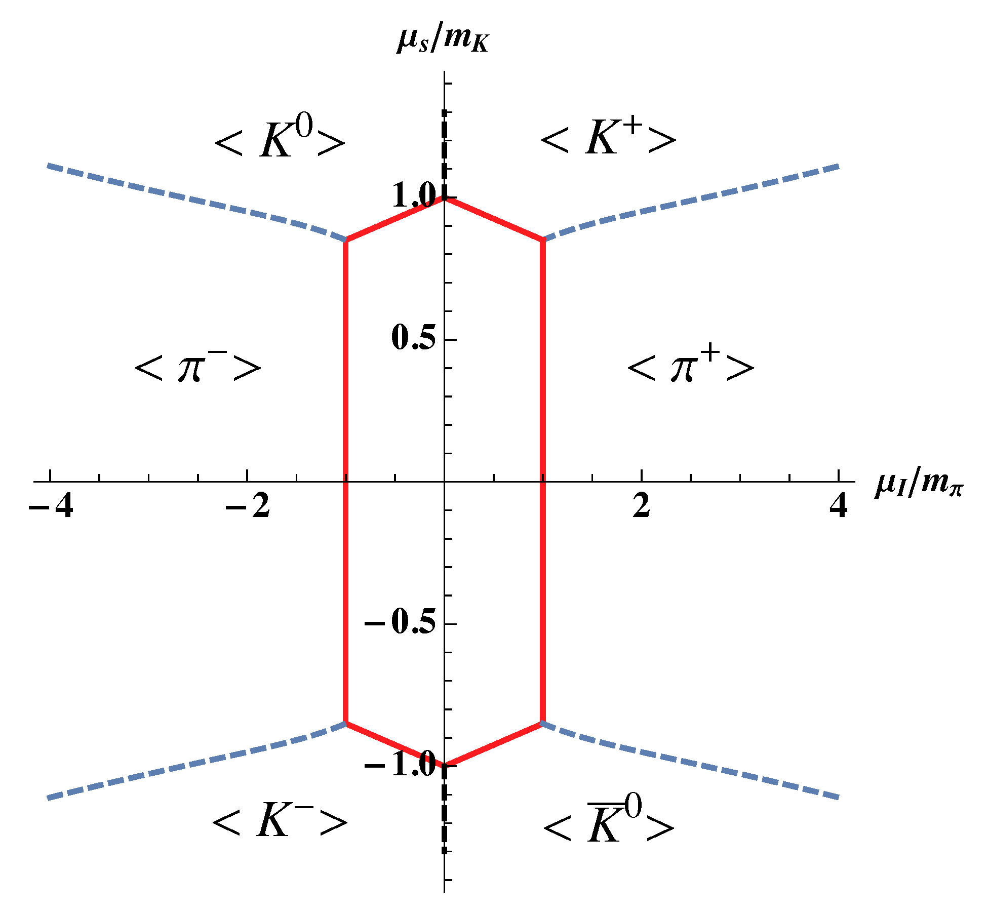
We can figure out the conditions for the final SSB of Figure 3 by inspecting the meson mass spectrum. The isospin and strangeness chemical potentials remove the degeneracy within isomultiplets and between states with different hypercharge. Since

$$[\mathcal{H},T_3]=0\mathrm{and}[\mathcal{H},T^2]=0,$$

(36)

in the normal phase we can still group eigenstates as isospin multiplets. By the lemmas of Schur, these states will not be degenerate in mass: there is a mass splitting within members of isomultiplets, proportional to ${\mu }_I$, and there is a mass splitting between states with different hypercharge, proportional to ${\mu }_S$. The only unaffected states are the ${\pi }_0$ and $\eta$ states, because they have both vanishing isospin and hypercharge. Since the mass splitting is given by the corresponding charges we have that

$$\begin{array}{cc}\hfill m_{{\pi }^0}& =m_{\pi },\hfill \end{array}$$

(37)

$$\begin{array}{cc}\hfill m_{{\pi }^{\pm }}& =m_{\pi }\mp {\mu }_I,\hfill \end{array}$$

(38)

$$\begin{array}{cc}\hfill m_{\eta }& =\sqrt{\frac{4m_K^2-m_{\pi }^2}{3}},\hfill \end{array}$$

(39)

$$\begin{array}{cc}\hfill m_{K^{\pm }}& =m_K\mp \frac{1}{2}{\mu }_I\mp {\mu }_S,\hfill \end{array}$$

(40)

$$\begin{array}{cc}\hfill m_{K^0/{\overline{K}}^0}& =m_K\pm \frac{1}{2}{\mu }_I\mp {\mu }_S,\hfill \end{array}$$

(41)

where $m_{\pi }$ and $m_K$ indicate the meson masses for ${\mu }_I={\mu }_S=0$.

To elucidate the mass splittings we show on the right of Figure 4 the results obtained for ${\mu }_I=80$ MeV and ${\mu }_S=90$ MeV. As discussed above, the first mass splitting is induced by the nonvanishing quark masses. The second splitting is due to the considered values of the chemical potentials, which completely remove the level degeneracies. The shown hierarchy is only one of the possible ones: different values of ${\mu }_I$ and/or ${\mu }_S$ may imply different level splittings, possibly with kaons lighter than pions.

The pion masses are independent of ${\mu }_S$ and we see from Equation (38) that for

$${\mu }_I=\left|m_{\pi }\right|,$$

(42)

one of the charged mesons becomes massless. Analogously, for $|{\mu }_S|=m_K-\left|{\mu }_I\right|/2$ one of the kaons becomes massless. The normal phase will persists until no mode is massless, that is for

$$|{\mu }_I|<m_{\pi }\mathrm{and}\left|{\mu }_S\right|<m_k-\frac{|{\mu }_I|}{2},$$

(43)

which corresponds to the irregular hexagon (solid red line) in Figure 5.

This phase diagram was first derived in [11] in the $\chi$PT framework. At the boundary of the hexagon we expect a massless mode, signaling a SSB. This massless mode eventually condenses if the temperature is below the relevant critical temperature. When meson condensation occurs, the vacuum will have a nonvanishing charge associated to one of the non-diagonal generators of $SU\left(3\right)$ characterizing the condensed meson.

For the description of the broken phases, we first note that the ${\mu }_I$ and ${\mu }_S$ Lagrangian terms are proportional to $T_3$ and $T_8$, respectively, see Equation (6). Since these two generators form the Cartan subalgebra of $SU\left(3\right)$, it turns out useful to consider the three $\mathcal{SU}\left(2\right)$ Lie subalgebras of $\mathcal{SU}\left(3\right)$ generated by

$$\begin{array}{c}\hfill T_{\pm },T_3,V_{\pm },V_3,U_{\pm },U_3,\end{array}$$

(44)

where the step operators are respectively

$$\begin{array}{c}\hfill T_{\pm }=T_1\pm i{T}_2,V_{\pm }=T_4\pm i{T}_5,U_{\pm }=T_6\pm i{T}_7,\end{array}$$

(45)

and

$$\begin{array}{c}\hfill Y=\frac{2}{\sqrt{3}}{T}_8,K=T_3-\frac{1}{\sqrt{3}}{T}_8,Q=T_3+\frac{1}{\sqrt{3}}{T}_8,\end{array}$$

(46)

are the corresponding weights.

Let us now consider the case in which one of the charged pions, say the ${\pi }^{+}$, becomes massless and condenses. The spontaneously broken generator is $T_{+}$, which locks the phases of up and down quarks. Since $[T_{+},Y]=0$, it follows the SSB

$$\underset{{\displaystyle \supset U{\left(1\right)}_Q}}{\underbrace{U{\left(1\right)}_I\times U{\left(1\right)}_Y}}\times U{\left(1\right)}_B\to \underset{{\displaystyle \not\supset U{\left(1\right)}_Q}}{\underbrace{U{\left(1\right)}_Y\times U{\left(1\right)}_B}},$$

(47)

meaning that the massless mode is the NGB associated to $U{\left(1\right)}_I$ breaking. We remark that this superfluid mode actually signals the transition to a superconducting phase, because the $U{\left(1\right)}_Q$ symmetry is broken. Since $[T_{+},Q]\ne 0$ the charged pion states can mix and indeed the massless mode coincides with the ${\pi }_{+}$ only at the phase transition point. In general it will be a superposition of the two charged pion states. Analogous results hold if the ${\pi }^{-}$ becomes massless and condenses, with $T_{-}$ the broken generator.

The second possibility is that the $K^{+}$ becomes massless and condenses; the spontaneously broken generator is $V_{+}$, which locks the phases of up and strange quarks. In this case $[V_{+},K]=0$, with the resulting SSB

$$\underset{{\displaystyle \supset U{\left(1\right)}_Q}}{\underbrace{U{\left(1\right)}_I\times U{\left(1\right)}_Y}}\times U{\left(1\right)}_B\to \underset{{\displaystyle \not\supset U{\left(1\right)}_Q}}{\underbrace{U{\left(1\right)}_K\times U{\left(1\right)}_B}},$$

(48)

meaning that there is a residual global symmetry associated to the weight K. In this case the isospin and hypercharge phases are locked. The system is a kaon superconductor, because the condensed meson is charged. Analogous results hold if the $K^{-}$ becomes massless and condenses.

The third case is the condensation of one of the neutral kaons. If the $K^0$ becomes massless and condenses, then the spontaneously broken generator is $U_{+}$, with down-strange quark phase locking. Since $[U_{+},Q]=0$, the resulting SSB is

$$\underset{{\displaystyle \supset U{\left(1\right)}_Q}}{\underbrace{U{\left(1\right)}_I\times U{\left(1\right)}_Y}}\times U{\left(1\right)}_B\to U{\left(1\right)}_Q\times U{\left(1\right)}_B,$$

(49)

meaning that the electromagnetic gauge field is unbroken. Therefore, the system is a kaon superfluid where the superfluid mode is given by the mixing of the two neutral kaons.

Let us analyze the order of the transition lines in Figure 5. The $\chi$SB and the meson condensation mechanisms are independent: the $\chi$SB is related to the locking of the phases of left- and right-handed quarks, while the meson condensation locks the phases of quarks with different flavors. This means that the chiral condensate and the meson condensate can coexist, therefore the irregular hexagon should be a second order phase transition line. On the other hand, it is not possible to have the simultaneous condensation of say ${\pi }^{+}$ and $K^{+}$ because both condensates involve an up quark. In group theory this is related to the fact that the two generators $T_{+}$ and $V_{+}$ do not commute. We expect that the presence of a meson condensate excludes the other, implying the first order phase transition shown in Equation (5) as dashed lines. The simultaneous condensation can only happen at the vertices of the hexagon or close to the first order phase transition lines if inhomogeneous phases are realized. This has been preliminarily explored by canonical LQCD simulation in [75] and by $\chi$PT in [30].

To summarize, any meson condensate tilts the vacuum in a certain direction having a residual $U{\left(1\right)}_B\times U\left(1\right)$ symmetry which is generated by the baryonic charge and by one of the weight operators in Equation (46). The low-energy spectrum consists of one NGB. This NGB has the same quantum numbers of one of the standard mesons at the phase transition point, but then in the superfluid phase it mixes with its charged conjugated state as shown in Figure 6, see also [26].

4. Modern Approaches

We now present two different approaches to the meson condensation, one is based on the effective field theory $\chi$PT description of mesons, the second on the NJL modelization of the strong interaction by a contact term. Then we compare the results of these methods with those of the pertinent LQCD numerical simulations. We restrict to consider an homogeneous and static medium; for inhomogeneous phases see [7,61,93,94,95].

4.1. Chiral Perturbation Theory

The $\chi$PT Lagrangian is an extremely powerful tool for systematically describe the strong interactions between hadrons [96,97,98,99,100,101,102,103,104]. Remarkably, $\chi$PT can also be used to study a variety of gauge theories with isospin asymmetry, including 2 color QCD with different flavors [105,106,107,108,109,110,111]. Quite generally, any $\chi$PT realization is based on two key ingredients: the global symmetries of the studied theory and an appropriate low momentum expansion.

The relevant global symmetry of QCD for constructing the $\chi$PT Lagrangian is the chiral symmetry

$$SU{\left(N_f\right)}_L\times SU{\left(N_f\right)}_R,$$

(50)

with $N_f$ the number of relevant quark flavors. The meson fields are collected in the unimodular $\Sigma$ field, transforming as

$$\Sigma \to L\Sigma R^{†},$$

(51)

where $L\in SU{\left(N_f\right)}_L$ and $R\in SU{\left(N_f\right)}_R$. Based on the chiral symmetry and this transformation property one builds the most general Lagrangian at the given order in the momentum expansion, assuming that the meson momenta satisfy

$$p\ll {\Lambda }_{\chi },$$

(52)

where ${\Lambda }_{\chi }\sim 1$ GeV is the $\chi$PT breaking scale. At each order in the momentum expansion the chiral symmetry fixes the form of the various Lagrangian pieces but the pre-factors, the so-called low energy constants (LECs), must be determined by different means. The leading $\mathcal{O}\left(p^2\right)$ $\chi$PT Lagrangian [11,97,103] describing the in-medium pseudoscalar mesons is given by

$$\mathcal{L}=\frac{f_{\pi }^2}{4}\mathrm{Tr}({\mathcal{D}}_{\nu }\Sigma {\mathcal{D}}^{\nu }{\Sigma }^{†})+\frac{f_{\pi }^2}{4}\mathrm{Tr}(X{\Sigma }^{†}+\Sigma X^{†}),$$

(53)

where the trace is in flavor space and the auxiliary field X transforms as $\Sigma$. The locking of the chiral rotations to the vector $SU{\left(N_f\right)}_V$ group is induced by the vev of X, see for example the discussion in [98,103], which is usually written as $\langle X\rangle =2BM$ with M the quark mass matrix defined in Equation (3). The two LECS, B and $f_{\pi }$, can be fixed by the vacuum properties [97,99,100,103,104]; for instance B from the mass relations $m_{\pi }^2=2Bm$ and $m_K^2=B(m+m_s)$, while $f_{\pi }\simeq 93$ MeV from the weak pion decays.

The adjoint covariant derivative in Equation (53) takes into account the minimal coupling of the meson fields with gauge fields, external currents and the effect of different chemical potentials [97,99,101]. Pretty much as the covariant derivative in the quark sector, see Equation (4), we define it as

$${\mathcal{D}}_{\nu }\Sigma ={\partial }_{\nu }\Sigma +\frac{i}{2}[v_{\nu },\Sigma ],$$

(54)

where the external current, $v_{\nu }$, is given in Equation (5); here we can take $\mu =\mathrm{diag}({\mu }_I/2,-{\mu }_I/2,-{\mu }_S)$ because mesons have no baryonic charge. This leading order (LO) $\chi$PT Lagrangian is sufficient to accurately describe the phase structure of QCD at ${\mu }_I\lesssim 2m_{\pi }$ [10,11,29], including finite temperature effects [22,23,24] and pion in-medium stability [26,28].

4.1.1. Ground State

The ground state can be variationally determined by replacing $\Sigma \to \overline{\Sigma }$ in Equation (53), where $\overline{\Sigma }$ is the time independent and homogeneous vacuum expectation value of the meson fields. The resulting static Lagrangian

$${\mathcal{L}}_{\mathrm{static}}=-\frac{f_{\pi }^2}{4}\mathrm{Tr}\left(\left[\mu ,\overline{\Sigma }\phantom{{}^{†}}\right]\left[\mu ,{\overline{\Sigma }}^{†}\right]\right)+\frac{f_{\pi }^{2}B}{2}\mathrm{Tr}\left(M(\overline{\Sigma }+{\overline{\Sigma }}^{†})\right),$$

(55)

must be maximized to determine the vacuum configuration. Specifically, one can parameterize the most general $SU\left(3\right)$ vev as

$$\overline{\Sigma }=e^{i\alpha \mathit{n}·\mathit{\lambda }},$$

(56)

where ${\lambda }_i$, for $i=1,\dots ,8$ are the Gell-Mann matrices, and the tilting angle $\alpha$ and the eight-dimensional unit vector $\mathit{n}$ are the variational parameters that should be obtained maximizing Equation (55). The normal phase is easily described by $\alpha =0$, thus $\overline{\Sigma }={\overline{\Sigma }}_N=I$, but in general one should maximize Equation (55) with respect to eight independent parameters, which is a rather formidable task. As far as I know, nobody has ever considered this procedure, and for a good reason. From the insight gained in Section 3 by the group theory analysis, we expect that in each different meson condensed phase the vacuum is rotated in a specific way. In the pion condensed phase the only nonvanishing components should be $(n_1,n_2)$, in the charged kaon condensed phase $(n_4,n_5)$, while in the neutral kaon condensed phase $(n_6,n_7)$. One can further simplify the ansatz observing that the potential must have a flat direction, the one spanned by the NGB.

To elucidate these aspects let us first focus on the $N_f=2$ case, with the most general ansatz

$$\overline{\Sigma }=e^{i\alpha \mathit{n}·\mathit{\sigma }}=cos\alpha +i\mathit{n}·\mathit{\sigma }sin\alpha ,$$

(57)

where $\mathit{n}=(n_1,n_2,n_3)$. The static Lagrangian now reads

$${\mathcal{L}}_{\mathrm{static}}=f_{\pi }^2{m}_{\pi }^{2}cos\alpha +\frac{f_{\pi }^2}{2}{(sin\alpha )}^2{\mu }_I^2(1-n_3^2),$$

(58)

showing that it is independent of $n_1$ and $n_2$, corresponding to the flat direction spanned by the NGB that interpolates between the ${\pi }_{+}$ and ${\pi }_{-}$ fields, see Section 3. For maximizing the Lagrangian one has to take $n_3=0$, then we have the freedom to take say $n_1=0$ and $n_2=1$. In summary, the ground state has vanishing projection along the isospin direction while the rotations around the direction of the chemical potential leave the vacuum invariant.

We now return to the three-flavor case. In the three different meson condensed phases we expect that it suffices to take only one entry of the unit vector $\mathit{n}$ nonzero. In particular, in the pion condensed phase

$$\begin{array}{cc}\hfill {\overline{\Sigma }}_{\pi }& =e^{i\alpha {\lambda }_2}=\left(\begin{array}{ccc}cos\alpha & sin\alpha & 0\\ -sin\alpha & cos\alpha & 0\\ 0& 0& 1\end{array}\right)=\frac{1+2cos\alpha }{3}I+i{\lambda }_{2}sin\alpha +\frac{cos\alpha -1}{\sqrt{3}}{\lambda }_8,\hfill \end{array}$$

(59)

while in the charged kaon condensed phase

$$\begin{array}{cc}\hfill {\overline{\Sigma }}_K=& e^{i\alpha {\lambda }_5}=\left(\begin{array}{ccc}cos\alpha & 0& sin\alpha \\ 0& 1& 0\\ -sin\alpha & 0& cos\alpha \end{array}\right)=\frac{1+2cos\alpha }{3}I+\frac{cos\alpha -1}{2\sqrt{3}}\left(\sqrt{3}{\lambda }_3-{\lambda }_8\right)+i{\lambda }_{5}sin\alpha ,\hfill \end{array}$$

(60)

finally in the neutral kaon condensed phase

$$\begin{array}{cc}\hfill {\overline{\Sigma }}_{K_0}=& e^{i\alpha {\lambda }_7}=\left(\begin{array}{ccc}1& 0& 0\\ 0& cos\alpha & sin\alpha \\ 0& -sin\alpha & cos\alpha \end{array}\right)=\frac{1+2cos\alpha }{3}I+\frac{1-cos\alpha }{2\sqrt{3}}\left(\sqrt{3}{\lambda }_3+{\lambda }_8\right)+i{\lambda }_{7}sin\alpha ,\hfill \end{array}$$

(61)

where $\alpha$ assumes different values in the three different phases.

To allow the transition between the three phases one can consider the more general ansatz

$$\overline{\Sigma }=e^{-i\gamma {\lambda }_2}{e}^{-i\beta {\lambda }_7}{e}^{i\alpha {\lambda }_2}{e}^{i\beta {\lambda }_7}{e}^{i\gamma {\lambda }_2},$$

(62)

with $\alpha ,\beta ,\gamma \in [0,\pi /2]$ are three different angles. Once again, the normal phase corresponds to $\alpha =0$ and it is insensitive to the values of $\beta$ and $\gamma$. The pion condensed phase corresponds to $\beta =0,\gamma =0$, the $K^{+}$ condensed phase to $\beta =\pi /2,\gamma =0$, the $K^0$ condensed phase to $\beta =\pi /2,\gamma =\pi /2$. Any value of $\beta$ and $\gamma$ different from the above ones indicates a phase with simultaneous condensation of two or more meson fields. We have argued in Section 3 that this is not the case. This has been explicitly shown in $\chi$PT for the ${\pi }^{+}$ and $K^{+}$ condensation phases [11]. In this case we can simplify the ground state ansatz by taking $\gamma =0$ in Equation (62), obtaining the same ansatz of [11]. Any value $\beta \in (0,\pi /2)$ corresponds to the simultaneous ${\pi }^{+}$-$K^{+}$ condensation. The analysis of [11] shows that at the phase transition the angle $\beta$ discontinuously jumps from 0 to $\pi /2$ resulting in a first order phase transition (as depicted in Figure 5): no simultaneous condensation is possible.

Below we summarize the main properties of the possible phases obtained by the $\chi$PT analysis. The phase diagram is in agreement with Figure 5, indeed it was first derived by $\chi$PT in [11]. Given the symmetry of the phase diagram we focus on the ${\mu }_I>0$ and ${\mu }_S>0$ part of Figure 5 characterized by the ${\pi }^{+}$ and $K^{+}$ condensates. The red solid line is exactly determined, while the $\chi$PT prediction for the dashed blue line is

$${\mu }_S=\frac{-m_{\pi }^2+\sqrt{{(m_{\pi }^2-{\mu }_I^2)}^2+4m_K^2{\mu }_I^2}}{2{\mu }_I}.$$

(63)

We also report below the relevant thermodynamic quantities. Once $\overline{\Sigma }$ is determined, the pressure is obtained from

$$P=-{\mathcal{L}}_{\mathrm{static}}\left(\overline{\Sigma }\right),$$

(64)

and then the number densities and the energy density follow from the thermodynamic relations

$$\begin{array}{c}\hfill n_{I,S}=\frac{\partial P}{\partial {\mu }_{I,S}},ϵ={\mu }_I{n}_I+{\mu }_S{n}_S-P.\end{array}$$

(65)

Finally one can obtain the equation of state (EoS) by appropriately expressing the chemical potentials as a function of the pressure.

• The normal phase is favored for

  $$\begin{array}{cc}\hfill {\mu }_I& <m_{\pi },\hfill \\ \hfill {\mu }_S& <m_K-\frac{1}{2}{\mu }_I,\hfill \end{array}$$

  (66)

  with the trivial vev ${\overline{\Sigma }}_N=\mathrm{diag}(1,1,1)$. The nonvanishing condensates are the three chiral condensates, see Equation (7),

  $${\sigma }_u={\sigma }_d={\sigma }_s\equiv {\sigma }_0,$$

  (67)

  where the subscript indicates the quark flavor and ${\sigma }_0$ is the value of the chiral condensate in vacuum. In the normal phase the values of the chiral condensates are not affected by the chemical potentials. The pressure is given by

  $$\begin{array}{c}\hfill P=\left\{\begin{array}{cc}{f}_{\pi }^2{m}_{\pi }^2\hfill & \mathrm{for}{N}_f=2,\hfill \\ f_{\pi }^2{m}_{\pi }^2\left(\frac{1}{2}+\frac{m_K^2}{m_{\pi }^2}\right)\hfill & \mathrm{for}{N}_f=3,\hfill \end{array}\right.\end{array}$$

  (68)

  and thus the isospin and strangeness number densities vanish, that is

  $$n_I=n_S=0.$$

  (69)
• The ${\pi }^{+}$ condensed phase is favored for

  $$\begin{array}{cc}\hfill {\mu }_I& >m_{\pi },\hfill \\ \hfill {\mu }_S& <\frac{-m_{\pi }^2+\sqrt{{(m_{\pi }^2-{\mu }_I^2)}^2+4m_K^2{\mu }_I^2}}{2{\mu }_I},\hfill \end{array}$$

  (70)

  resulting in the vacuum in Equation (59) with

  $$cos{\alpha }_{\pi }={\left(\frac{m_{\pi }}{{\mu }_I}\right)}^2,$$

  (71)

  determined by maximizing the static Lagrangian in Equation (58). The condensates are given by

  $$\begin{array}{cc}\hfill {\sigma }_u& ={\sigma }_d={\sigma }_{0}cos{\alpha }_{\pi }{\sigma }_s={\sigma }_0\hfill \\ \hfill \langle {\pi }^{+}\rangle & ={\sigma }_{0}sin{\alpha }_{\pi }\langle K^{+}\rangle =0,\hfill \end{array}$$

  (72)

  and the pressure produced by the condensation of pions is given by [10,11]

  $$P=\frac{f_{\pi }^2{\mu }_I^2}{2}{\left(1-\frac{m_{\pi }^2}{{\mu }_I^2}\right)}^2,$$

  (73)

  where the normal phase pressure has been subtracted. This expression is valid for both $N_f=2$ and $N_f=3$; it is of course insensitive to the kaon mass and the strange quark chemical potential. The number densities are

  $$\begin{array}{c}\hfill n_I=f_{\pi }^2{\mu }_I\left(1-\frac{m_{\pi }^4}{{\mu }_I^4}\right)n_s=0,\end{array}$$

  (74)

  and the $\mathcal{O}\left(p^2\right)$ equation of state [27] is

  $$ϵ\left(P\right)=-P+2\sqrt{P(2f_{\pi }^2{m}_{\pi }^2+P)}.$$

  (75)
• The $K^{+}$ condensed phase is favored for

  $$\begin{array}{cc}\hfill {\mu }_S& >m_K-\frac{1}{2}{\mu }_I,\hfill \\ \hfill {\mu }_S& >\frac{-m_{\pi }^2+\sqrt{{(m_{\pi }^2-{\mu }_I^2)}^2+4m_K^2{\mu }_I^2}}{2{\mu }_I},\hfill \end{array}$$

  (76)

  resulting in the vacuum in Equation (60) with

  $$cos{\alpha }_K={\left(\frac{m_K}{{\mu }_K}\right)}^2,$$

  (77)

  where ${\mu }_K={\mu }_I/2+{\mu }_S$ is the relevant combination of chemical potentials, because $K^{+}$ has isospin $1/2$ and strangeness 1. The condensates are given by

  $$\begin{array}{cc}\hfill {\sigma }_u& ={\sigma }_s={\sigma }_{0}cos{\alpha }_K{\sigma }_d={\sigma }_0\hfill \\ \hfill \langle {\pi }^{+}\rangle & =0\langle K^{+}\rangle ={\sigma }_{0}sin{\alpha }_K,\hfill \end{array}$$

  (78)

  and the normalized pressure by

  $$P=\frac{f_{\pi }^2{\mu }_K^2}{2}{\left(1-\frac{m_K^2}{{\mu }_K^2}\right)}^2,$$

  (79)

  which consents to obtain the number densities

  $$\begin{array}{c}\hfill n_I=\frac{f_{\pi }^2{\mu }_K}{2}\left(1-\frac{m_K^4}{{\mu }_K^4}\right)n_s=2n_I.\end{array}$$

  (80)
  The EoS is

  $$ϵ\left(P\right)=-P+2\sqrt{P(2f_{\pi }^2{m}_K^2+P)}.$$

  (81)

As we shall see in Section 4.3, these $\chi$PT results are in good agreement with the NJL and LQCD results close to the second order phase transitions.

Let us briefly comment on the difference between the charged meson condensed phases and the neutral kaon condensed phase. The expression of the various thermodynamic quantities in the neutral kaon condensed phase can be obtained from those of the charged kaon condensed phase by replacing ${\mu }_I\to -{\mu }_I$, due to the fact that $K_0$ has isospin $-1/2$. The relevant difference, as we have already noted is Section 3, is that the $K_0$ and the ${\overline{K}}_0$ condensed phases are superfluid, while the charged meson condensed phases are superconductors. In the latter case one can determine the screening masses of the electromagnetic field by gauging the $U{\left(1\right)}_Q$ subgroup of the chiral group, see Equation (30), resulting in the Debye and Meissner screening masses [26]

$$M_D^2=M_M^2=f_{\pi }^2{e}^2{(sin\alpha )}^2,$$

(82)

where the Debye mass is related to the electric charge susceptibility, see for instance [112], while the nonvanishing value of the Meissner mass implies that the system is a superconductor.

4.1.2. Low-Energy Excitations

Once the ground state has been identified, one can determine the low-energy fluctuations by an appropriate expansion. This is quite useful also because it allows us to identify the NGB. We briefly illustrate the procedure for the two-flavor case. A useful parameterization is

$$\Sigma =cos\rho +i\widehat{\mathit{\phi }}·\mathit{\sigma }sin\rho ,$$

(83)

where the radial field, $\rho$, and the unit vector field, $\widehat{\mathit{\phi }}$, encode in a nontrivial way the three pion fields. By this parameterization the LO $\chi$PT Lagrangian takes the form obtained in [29]

$$\begin{array}{cc}\hfill \mathcal{L}=& \frac{f_{\pi }^2}{2}\left({\partial }^{\mu }\rho {\partial }_{\mu }\rho +{sin}^2\rho {\partial }^{\mu }{\widehat{\phi }}_i{\partial }_{\mu }{\widehat{\phi }}_i-2m_{\pi }\gamma {sin}^2\rho {ϵ}_{3ik}{\widehat{\phi }}_i{\partial }_0{\widehat{\phi }}_k\right)-V\left(\rho \right),\hfill \end{array}$$

(84)

where

$$V\left(\rho \right)=-f_{\pi }^2{m}_{\pi }^2\left(cos\rho +\frac{{\gamma }^2}{2}{sin}^2\rho \right),$$

(85)

is the potential and $\gamma ={\mu }_I/m_{\pi }$ is the control parameter. From the ground state analysis we know that the pion condensed phase is favored for $\left|\gamma \right|>1$, and the minimum of the potential is attained for the radial field vev, $\overline{\rho }={\alpha }_{\pi }$, see Equation (71).

The low-energy radial and angular excitations can now be introduced as follows [26,29,30]

$$\rho ={\alpha }_{\pi }+\chi ,\widehat{\mathit{\phi }}=({\phi }_1,{\phi }_2),$$

(86)

where we have neglected the fluctuation of the ${\phi }_3\equiv {\pi }_0$ field, because it decouples. We can parameterize the angular field by

$$\widehat{\mathit{\phi }}=(cos\theta ,sin\theta ),$$

(87)

where $\theta$ is the Bogolyubov mode, and rescaling the radial field as $\chi \to \chi /f_{\pi }$ and the Bogolyubov mode as $\theta \to \theta /f_{\pi }sin\overline{\rho }$, one obtains the quadratic Lagrangian

$$\mathcal{L}=\frac{1}{2}{\partial }^{\mu }\chi {\partial }_{\mu }\chi -\frac{1}{2}{m}_{\chi }^2{\chi }^2+\frac{1}{2}{\partial }_{\mu }\alpha {\partial }^{\mu }\alpha -g\chi {\partial }_0\alpha ,$$

(88)

where $m_{\chi }=m_{\pi }\gamma sin{\alpha }_{\pi }$ is the mass of the radial field fluctuations and $g=2{\mu }_I$ is the coupling between the oscillations of the radial and the angular fields. The mass of the radial mode vanishes at the phase transition to the normal phase because it is a second order phase transition. The Bogolyubov field seems to propagate at the speed of light, but integrating out the radial fluctuations one obtains the actual NGB with a phonon-like dispersion law

$$\begin{array}{cc}\hfill E_{\mathrm{ph}}& =c_{s}p,\hfill \end{array}$$

(89)

thus propagating at the sound speed [10],

$$\begin{array}{cc}\hfill c_s& =\sqrt{\frac{\partial P}{\partial n_I}}=\sqrt{\frac{{\gamma }^4-1}{{\gamma }^4+3}}.\hfill \end{array}$$

(90)

Alternatively, by diagonalizing the quadratic Lagrangian one obtains the dispersion laws

$$\begin{array}{cc}\hfill E_{\pm }& =\sqrt{p^2+\frac{m_{\mathrm{eff}}^2}{2}\pm \sqrt{{\left(\frac{m_{\mathrm{eff}}^2}{2}\right)}^2+g^2{p}^2}},\hfill \end{array}$$

(91)

where the low momentum expansion of the $E_{-}$ field coincides with the NGB dispersion law and the other mode with mass

$$\begin{array}{cc}\hfill m_{\mathrm{eff}}^2& =m_{\chi }^2+g^2=m_{\pi }^2\frac{{\gamma }^4+3}{{\gamma }^2},\hfill \end{array}$$

(92)

is the rotated radial mode. In conclusion, the low-energy modes correspond to a NGB with dispersion law in Equation (89) and to a radial mode with mass $m_{\mathrm{eff}}$.

4.2. The Nambu-Jona Lasinio Model

The meson condensed phases can also be studied by a modeling of the strong interaction by contact interaction terms [34,35,36,37,38,39,40,41,45,46,47,50,52,55], see [54] for a brief recent review. These models stem from the original work by Nambu and Jona Lasinio [113,114,115] of a pre-QCD Lagrangian for the description of the strong interaction by contact interaction terms:

$$\begin{array}{c}\hfill \mathcal{L}=\overline{\psi }\left[i{\gamma }^{\mu }{\partial }_{\mu }-M\right]\psi +G[{\left(\overline{\psi }\psi \right)}^2+{\left(\overline{\psi }i{\gamma }_5\mathit{\sigma }\psi \right)}^2],\end{array}$$

(93)

where $\psi$ is the two-nucleon isodoublet, M is the pertinent mass matrix and G is a dimensional coupling. The interaction preserves the global symmetry group G, see Equation (30), for a proper description of hadronic matter. The nucleons emerge as quasiparticle states and the spontaneously breaking of the chiral symmetry leads to the appearance of mesons. The model is based on an analogy with the BCS theory of superconductivity describing the electron interaction by means of a local interaction term with no gauge fields. It is not completely specified until a regularization scheme is provided and the value of the coupling constant is fixed.

In the modern view [35,57,116,117,118], the model describes quark matter with an effective contact interaction term that preserve the chiral symmetries of QCD. The spinor $\psi$ in Equation (93) now represents the quark fields and M the corresponding mass matrix, see Equation (3). The NJL model (eventually supplemented by Polyakov loop terms) has been applied to study the entire QCD phase diagram in Figure 1. The major phenomenological shortcoming of the quark NJL model is that it does not provide a confinement mechanism, indeed it has no gauge dynamics. Moreover, the presence of a dimension 6 operator requires an ultra-violet regularization scheme [57], which in the most used approximations is a hard cutoff at the $\Lambda \sim 1$ GeV scale or a form factor of the form [119]

$$F\left({\mathit{p}}^2\right)=\frac{{\Lambda }^2}{{\mathit{p}}^2+{\Lambda }^2},$$

(94)

to mimic the asymptotic freedom property of QCD. The coupling constant and the bare quark masses are then fixed to reproduce the low energy physics. Typical values of these quantities are

$$G{\Lambda }^2\simeq 6m\simeq 1.5\mathrm{MeV}{m}_s\simeq 50\mathrm{MeV},$$

(95)

see however [57,118]. The NJL model is a useful tool for a qualitative and semiquantitative exploration of the properties of hadronic matter, however the obtained results depend on the choice of these parameters and on the regularization scheme employed. Unfortunately, one cannot systematically improve the model because no expansion parameter can be identified. Despite these limitations, the NJL Lagrangian is Lorentz invariant, with the chiral symmetry realized and spontaneously broken exactly as it is expected to happen in QCD: by a chiral condensate. Moreover, the chiral symmetry can be explicitly broken by the inclusion of small current quark masses.

There is a certain degree of uncertainty in the form of the NJL Lagrangian. In the two-flavor case most of the authors retain the form in Equation (93), although different chirally symmetric interactions can be written. This increases the number of phenomenological parameters that have to be fixed. Following [57,118,120], the NJL Lagrangian can be generalized to

$$\mathcal{L}=\overline{\psi }\left[i{\gamma }^{\mu }{\partial }_{\mu }-M\right]\psi +{\mathcal{L}}_1+{\mathcal{L}}_2,$$

(96)

where the two interaction terms are

$$\begin{array}{cc}\hfill {\mathcal{L}}_1& =G_1[{\left(\overline{\psi }\psi \right)}^2+{\left(\overline{\psi }i{\gamma }_5\mathit{\sigma }\psi \right)}^2+{\left(\overline{\psi }\mathit{\sigma }\psi \right)}^2+{\left(\overline{\psi }i{\gamma }_5\psi \right)}^2]\hfill \\ \hfill {\mathcal{L}}_2& =G_2[{\left(\overline{\psi }\psi \right)}^2+{\left(\overline{\psi }i{\gamma }_5\mathit{\sigma }\psi \right)}^2-{\left(\overline{\psi }\mathit{\sigma }\psi \right)}^2-{\left(\overline{\psi }i{\gamma }_5\psi \right)}^2].\hfill \end{array}$$

(97)

The first term preserves the $U{\left(1\right)}_A$ symmetry while the second term explicitly breaks it. Whether or not the latter is comparable with the first depends on nonperturbative effects, indeed the $U{\left(1\right)}_A$ breaking term is supposed to describe the interaction mediated by some instanton configurations of the gauge fields. Considering different values of the coupling constants $G_1$ and $G_2$ implies distinct values of the chiral condensates of different flavors and a different phase diagram. This issue emerges also in the three-flavor case, where the NJL Lagrangian takes a slightly different form [121],

$$\begin{array}{cc}\hfill \mathcal{L}=& \overline{\psi }\left[i{\gamma }^{\mu }{\partial }_{\mu }-M\right]\psi +G\sum _{a=0}^8[{\left(\overline{\psi }{\lambda }_a\psi \right)}^2+{\left(\overline{\psi }i{\gamma }_5{\lambda }_a\psi \right)}^2]-K[det\overline{\psi }(1+{\gamma }_5)\psi +det\overline{\psi }(1-{\gamma }_5)\psi ],\hfill \end{array}$$

(98)

where now ${\psi }^T=(u,d,s)$ and G and K are the two coupling constants analogous of $G_1$ and $G_2$; the determinant term removes the $U{\left(1\right)}_A$ symmetry. Considering the $U{\left(1\right)}_A$ symmetric Lagrangian with $K=0$, the authors of [36] find the same transition hexagon (solid red line) reported in Figure 5, however the up and down chiral condensates split and at large values of the chemical potentials they find phase transition lines not present in Figure 5.

In the following we will focus on the traditional two-flavor NJL model, with $G_1=G_2=G/2$ corresponding to the Lagrangian in Equation (93), and thus maximally violated $U{\left(1\right)}_A$ symmetry. The presence of a medium can be described by a covariant derivative analogous to Equation (4), which takes into account the baryon and isospin chemical potentials. With the NJL model one can explore the entire QCD phase diagram (with the limitations discussed above), a clear advantage with respect to the $\chi$PT approach which can hardly investigate the effect of the baryon chemical potential. To obtain the properties of the vacuum and of the low-energy excitations one can perform a Hubbard-Stratanovich transformation introducing the collective boson variables

$${\sigma }_f\left(x\right)=-\frac{4G}{\Lambda }\left({\overline{\psi }}_f{\psi }_f\right){\pi }_a=-\frac{2G}{\Lambda }(\overline{\psi }{\gamma }_{5}i{\lambda }_a\psi +\mathrm{h}.\mathrm{c}.),$$

(99)

corresponding to scalar and pseudoscalar fields. Their expectation values are determined by minimizing the one loop effective potential, or equivalently, by solving the coupled gap equations. By this analysis it has been confirmed that the pion condensed phase sets in at ${\mu }_I=m_{\pi }$, see [38]. Moreover, it has been determined the dependence of the condensates on the chemical potentials and on the temperature.

At vanishing temperature, in the two flavor case the grand potential has the particularly simple expression

$$\Omega =G({\sigma }^2+{\langle \pi \rangle }^2)-\frac{3}{2{\pi }^2}{\int }_0^{\Lambda }dk{k}^2(E_{+}+E_{-}),$$

(100)

where we have used the hard cutoff procedure and the quark quasiparticle dispersion laws are given by

$$\begin{array}{c}\hfill E_{q,\pm }=\sqrt{{\left(E_k\pm \frac{{\mu }_I}{2}\right)}^2+4G^2{\langle \pi \rangle }^2},\end{array}$$

(101)

where $E_k=\sqrt{k^2+{\overline{m}}^2}$ with $\overline{m}=m-2G\sigma$ the effective quark mass. Therefore, the effect of the chiral condensate is a shift of the quark masses [57], while the pion condensate opens a gap between the quasiparticle dispersion laws. This is the typical effect of condensation on the quasiparticle spectrum, as it indicates the formation of correlated pairs of fermions. In the pion condensed phase it costs additional energy to produce quasiparticle fermionic excitations because of quark-antiquark pairs. Clearly, this picture of meson condensation cannot be directly compared with the $\chi$PT results of the previous section, because the considered degrees of freedom are different. However, as we shall discuss below, the values of the pion and chiral condensates can be compared, as well as various thermodynamic quantities. Moreover, the three flavor NJL model phase diagram obtained in [38] is in agreement with the theory group expectation in Figure 5 and quantitatively very similar to that obtained in $\chi$PT.

In the NJL model it is possible to include an electron (or positron) background to neutralize the pion electric charge. When requiring the electrical neutrality [39,40], the NJL models tend to disfavor the appearance of the pion condensed phase [45,47]. At the physical point, corresponding to a neutral configuration in hydrostatic equilibrium, the pions do not condense [45].

4.3. Comparison with Lattice QCD

The LQCD simulations are numerical implementation of the QCD action on a discretized grid; the relevant physical results are then obtained performing the limit to the continuum. These simulations can lead to the precise determination of many hadronic quantities and can provide numerical evidence for conjectured properties of strongly interacting matter. The LQCD simulations have been very successfully used for simulating hadronic matter in vacuum, but dealing with in medium effects poses a series of problems. The most important one is that the LQCD simulations at finite baryonic density are hampered by the so-called sign problem. Very briefly, in the LQCD simulations with dynamical quarks the Dirac degrees of freedom are typically integrated out, see for instance [122,123], resulting in a partition function that can be written as the euclidean path integral

$$\mathcal{Z}\sim \int d{A}_{\mu }{e}^{-S\left(A_{\mu }\right)}det{\Delta }_D,$$

(102)

where S is the euclidean action, $A_{\mu }$ are the gauge fields and $det{\Delta }_D$ is the determinant of the Dirac operators. The standard Monte Carlo simulations are based on importance sampling of the possible gauge configurations. This procedure works if $det{\Delta }_D>0$, that is with a real and positive Euclidean path integral measure. At nonvanishing baryonic density the LQCD numerical technique becomes problematic because the Dirac determinant is complex. Although continuous progress for facing this problem has been reported over the years, see for example [124,125,126,127,128], as of yet it is not a feasible tool for exploring the QCD phase diagram at large ${\mu }_B$ and, in particular, the transition from the confined phase to the CSC phase in Figure 1. See however [68,129,130,131] for different LQCD approaches to the region with nonvanishing baryonic and isospin chemical potentials.

Since it is hard to manage baryons in LQCD simulations, people decided to ignore baryons. This poses the LQCD simulations outside the beta-equilibrated sheet, as discussed in Section 1, to explore a part of the QCD phase diagram where the outcomes of the numerical simulations can be compared with different methods, in particular with the $\chi$PT and the NJL results. The key point is indeed that the LQCD simulations at nonvanishing isospin chemical potential and zero baryonic density are not affected by the sign problem [68]. This does not mean that this direction is without obstacles: the realization of multi-hadron systems in LQCD is an extremely challenging problem, see [132] for a review. There is a wealth of LQCD results for the pion condensation [70,71,72,73,76,77,79,82] while there has been little progress on kaons [74,75]. As we will see, the LQCD results on pion condensation are reliable only for ${\mu }_I\le 2m_{\pi }$, but these simulations are steadily improving and becoming more accurate, even with physical quark masses and external magnetic fields [77,79,82]

The LQCD simulations can be performed in the canonical or in the grand canonical ensembles. In the grand canonical simulation one discretizes on a lattice the actual QCD Lagrangian in Equation (2) with the isospin chemical potential as external source. In this approach the strangeness density has to be zero, as the strangeness chemical potential makes the measure complex. Moreover, the QCD Lagrangian has to be supplemented with a pionic source [69,70]

$${\mathcal{L}}_{\lambda }=i\lambda \overline{\psi }{\gamma }_5{\sigma }_2\psi ,$$

(103)

to trigger the breaking of the $U{\left(1\right)}_I$ symmetry and to stabilize the numerical simulations. Since the $\lambda$ term explicitly breaks the $U{\left(1\right)}_I$ symmetry, in the pion condensed phase there is a pseudo-NGB with vanishing mass in the $\lambda \to 0$ limit. Therefore, the physical interesting results are obtained doing both the continuum and the $\lambda \to 0$ limits. The first quenched LQCD simulations [69] already reported the expected behavior of the condensates; these results were soon improved considering $N_f=2$ dynamical quarks in [70]. To obtain more precise results one has to consider that both the pion and the chiral condensates depend in a rather non-trivial way on $\lambda$. Moreover, the first simulations employed a large pion mass. Progress with respect to these aspects has been reported in [133] where the $\lambda \to 0$ limit has been tackled by a reweighing technique in simulations with 2 light flavors and a heavy strange quark at the physical pion mass.

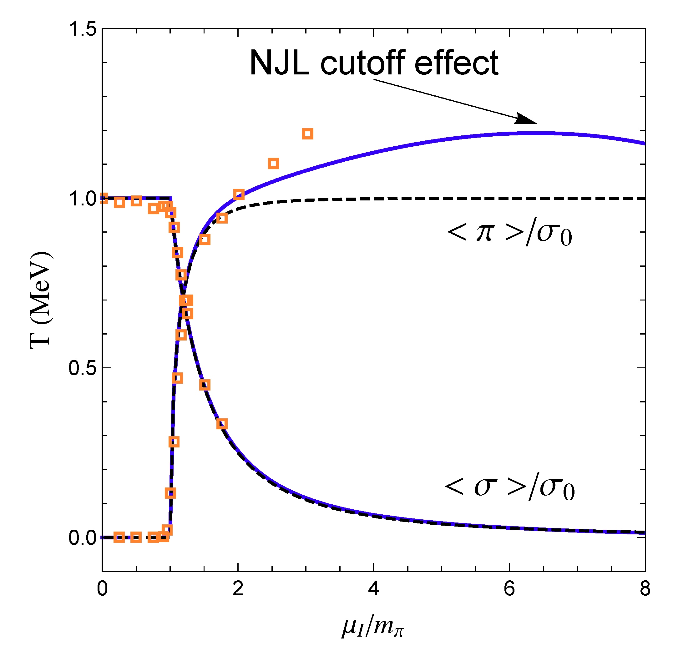
In Figure 7 we compare the pion and chiral condensates obtained by the LO $\chi$PT, see Section 4.1, by the two-flavor NJL model, see Section 4.2, and by the LQCD simulations of [133].

The chiral condensate obtained with the three approaches agree for any considered (or available) value of ${\mu }_I$. On the other hand, the pion condensates deviate at ${\mu }_I\sim 2m_{\pi }$. In $\chi$PT the the two condensates obey the relation

$${\sigma }^2+{\langle {\pi }^{+}\rangle }^2={\sigma }_0^2,$$

(104)

and therefore the pion condensate quickly saturates at ${\mu }_I\sim 2m_{\pi }$. Both the NJL and the LQCD results for the pion condensate indicate that it exceeds ${\sigma }_0$ and it does not saturate at ${\mu }_I\sim 2m_{\pi }$. This seems a robust result, although for larger values of ${\mu }_I$ both the NJL and the LQCD approaches become problematic. The NJL results show a non-monotonic behavior due to the hard cutoff $\Lambda$, which serves to mimic the asymptotic behavior of QCD, but that also signals the scale at which the NJL results are not under control. Similarly, the LQCD simulations feel the finite size lattice effects, indeed for large value of ${\mu }_I$ saturation effects become important, see for example [70]. Anyway, one can certainly regard this comparison as successful, in the sense that in the range ${\mu }_I\lesssim 2m_{\pi }$, where all the three approaches are supposed to work, they give very similar results.

We now turn to the canonical approach [73,74,75,76]. The canonical LQCD simulations can explore quark matter at nonvanishing isospin and strangeness density, while grand-canonical LQCD simulations can only deal with finite isospin density. In the canonical LQCD simulations the isospin and strangeness density are fixed and the corresponding chemical potentials are determined by thermodynamic relations. The description of mesons in the canonical LQCD simulation is attained by the introduction of external sources with a fixed isospin or strangeness charge. In these simulations the calculation of the meson field correlator requires the computation of a large number of Wick contraction of the quark fields on the lattice, leading to time consuming and expensive calculations. This is the main limitation of the canonical lattice simulations. Various different algorithms for reducing theses costs have been developed in [76], resulting in the simulation of up to $72{\pi }^{+}$ in configurations with spatial extents $L\sim 2,2.5$ and 3 fm, resulting in isospin chemical potentials up to $4.5m_{\pi }$ [76].

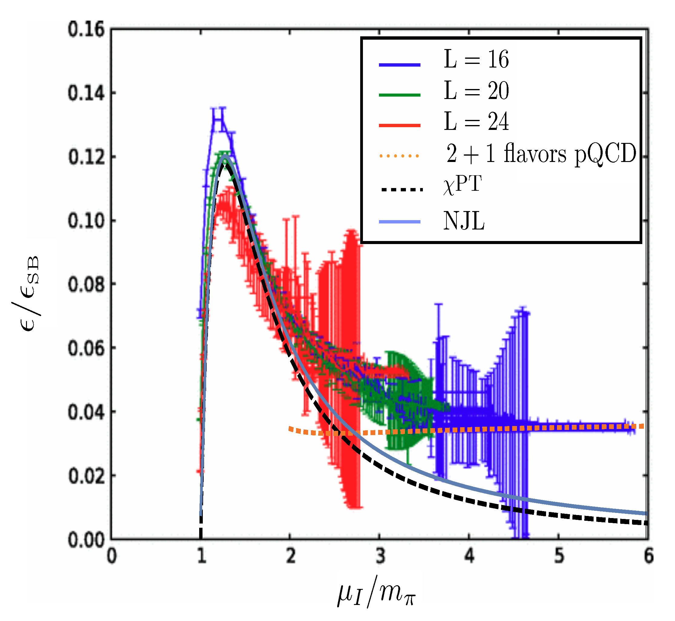
In Figure 8 we compare the energy density obtained with the canonical LQCD simulations with that of the $\chi$PT and the NJL approaches.

More precisely, in this figure it is shown the normalized energy density $ϵ/{ϵ}_{\mathrm{SB}}$, where ${ϵ}_{SB}=9{\mu }_I^4/\left(4{\pi }^2\right)$ is the Stefan-Boltzmann limit, as a function of the normalized isospin chemical potential, ${\mu }_I/m_{\pi }$. The dots with error bars are the results of [76] obtained with three different spatial volumes $L^3$. With increasing ${\mu }_I$ the error bars increase, signaling that lattice simulations cease to be reliable at ${\mu }_I\sim 2m_{\pi }$, as in the grand-canonical LQCD simulations discussed above. In this regime, the normalized energy well agrees with the $\chi$PT results (dashed black line), and with the NJL results (solid blue line). Both the $\chi$PT and the NJL curves perfectly capture the peak structure at low ${\mu }_I$, while they begin to depart from the LQCD results at ${\mu }_I\sim 2m_{\pi }$. The $\chi$PT and the NJL peak positions are respectively at

$$\begin{array}{cc}\hfill {\mu }_{I,\chi \mathrm{PT}}^{\mathrm{peak}}& ={\left(\sqrt{13}-2\right)}^{1/2}{m}_{\pi }\simeq 1.27m_{\pi },\hfill \end{array}$$

(105)

$$\begin{array}{cc}\hfill {\mu }_{I,\mathrm{NJL}}^{\mathrm{peak}}& \simeq 1.27m_{\pi },\hfill \end{array}$$

(106)

where the $\chi$PT results are independent of $f_{\pi }$, while the NJL results are not very sensitive to the parameter set used. The LQCD results of [76] are peaked at

$${\mu }_{I,\mathrm{LQCD}}^{\mathrm{peak}}=\{1.20,1.25,1.275\}{m}_{\pi },$$

(107)

where the different values are obtained for lattice sides $L=\{16,20,24\}$, respectively; the continuum-linearly-extrapolated peak is at ${\mu }_{I,\mathrm{LQCD}}^{\mathrm{peak}}\simeq 1.30m_{\pi }$. Therefore, also the canonical LQCD simulations are in agreement with the $\chi$PT and the NJL results for ${\mu }_I\lesssim 2m_{\pi }$.

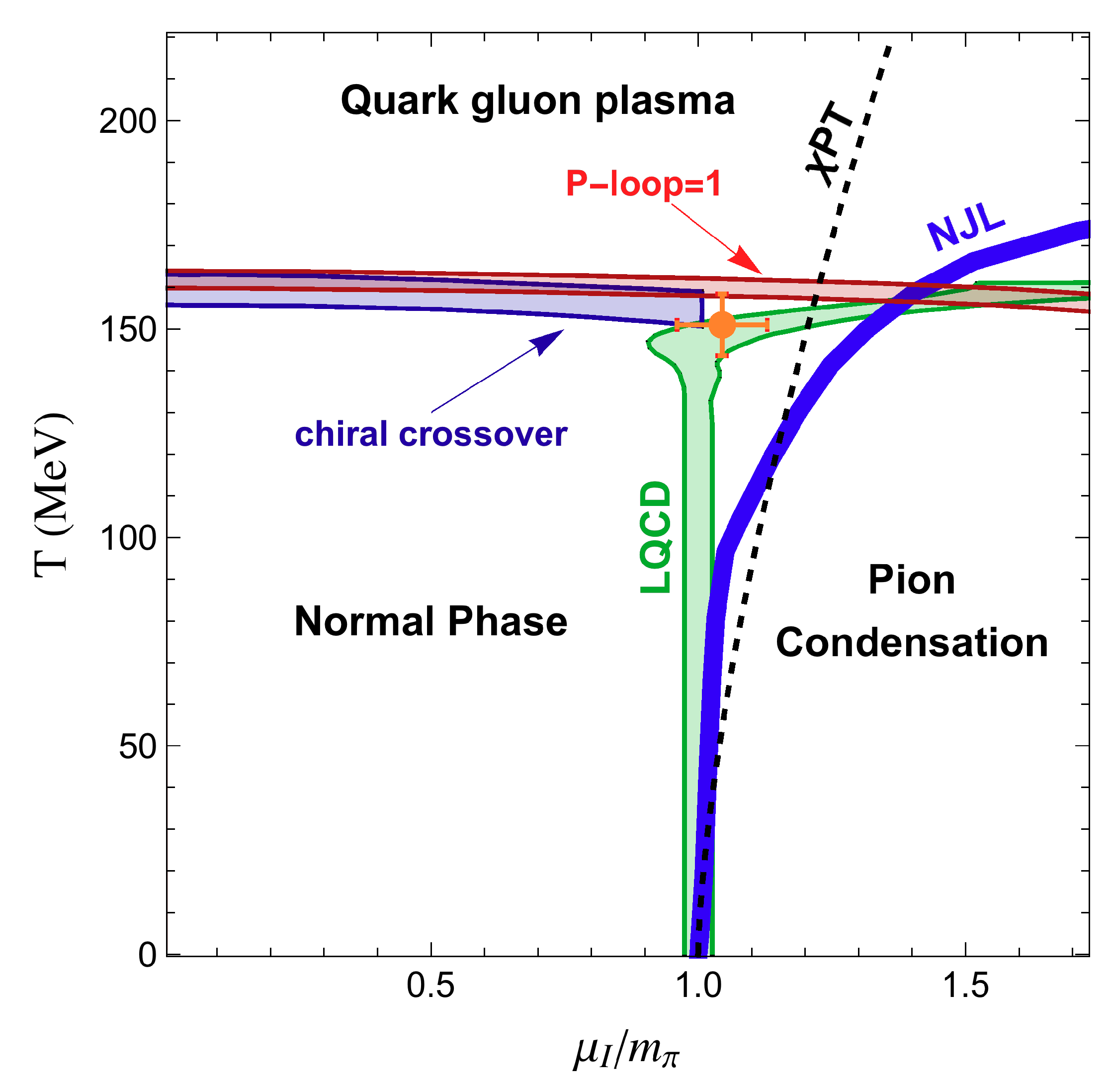
Nonvanishing Temperature

Given the successful comparison of the $\chi$PT, NJL and LQCD approaches at $T=0$, one may expect a similar agreement at small temperatures. As we will see, the agreement between the three methods at $T\ne 0$ is much worse. Herein we report on the investigation of the phase diagram at $T\ne 0$ and ${\mu }_I\ne 0$ comparing the results for the transition lines at ${\mu }_B=0$ separating the pion condensed phase from the normal phase at low T, and between the pion condensed phase and the quark-gluon plasma, at high T. We show in Figure 9 the results obtained with the different approaches. The LQCD simulations of [133] indicate that at ${\mu }_B=0$ there is in the ${\mu }_I,T$ plane a chiral crossover line (shaded blue region) joining the points $(0,160)$ to the (pseudo) tricritical point $(140,151)$ (orange dot with error bars). At the tricritical point the chiral crossover line joins the second order phase transition line (shaded green region). The LQCD results for the second order phase transition are almost insensitive to the temperature for $T\lesssim 150$ MeV, then the phase transition line becomes strongly temperature dependent, with a sort of “T-like” phase diagram shape. The mean-field NJL second order phase transition (solid blue line) [38] shows a behavior similar to that of the LQCD simulations for $T\lesssim 100$ MeV, then for higher temperatures the NJL results show a more pronounced temperature dependence. Eventually, the NJL critical curve saturates with a critical temperature that is not sensitive to the isospin chemical potential for $500\mathrm{MeV}<{\mu }_I<1$ GeV (not shown in the figure). The analytic $\chi$PT temperature dependence of the second order phase transition has been obtained in [22]

$${\mu }_I\left(T\right)=m_{\pi }+\frac{1}{4f_{\pi }^2}\sqrt{\frac{m_{\pi }^3{T}^3}{2{\pi }^3}}\zeta \left(\frac{3}{2}\right),$$

(108)

and is reported in Figure 9 with a dashed black line. The $T^{3/2}$ behavior does not agree with the LQCD nor with the NJL results. The $\chi$PT results of [24] indicate an even stronger temperature dependence. These results are somehow surprising, as one would expect $\chi$PT to work up to $T\lesssim 100$ MeV while Figure 9 shows that it is inconsistent with the LQCD low temperature behavior.

Given the rather precise LQCD data, one should understand what are the origins of the discrepancies. The NJL results have been obtained by a hard cutoff scheme, maybe one can relax this requirement by a Pauli-Villars regularization scheme or by a form factor, as in (94), that does not completely eliminate the hard scale contribution. The improved $\chi$PT results of [24] do not match the LQCD behavior at low ${\mu }_I$ but indicate a critical temperature that is independent of the chemical potential for ${\mu }_I>T$, which is in agreement with both the LQCD and NJL simulations. One should certainly try to understand what is the $\chi$PT missing ingredient at lower temperatures.

Quite remarkably, the LQCD simulations are now tackling the color deconfinement transition as a function of the isospin chemical potential. Color deconfinement can be characterized by the behavior of the so-called Polyakov loop, see for instance [4,134],

$$P\left(r\right)=\frac{1}{3}\mathrm{Tr}{\Pi }_{\tau =1}^{N_{\tau }}{U}_{\tau }\left(r\right),$$

(109)

at large lattice spacing. The expectation value of the Polyakov loop is related to the correlation function between two static heavy quarks, therefore it is a measure of the strength of the color interaction. It has the important property to vanish in the color confined phase of pure gauge theories [4]. A first inspection of the Polyakov loop dependence at nonvanishing ${\mu }_I$ and T has been done in [133], by a ${24}^3\times 6$ lattice. Various lines of constant values of the Polyakov loop have been obtained to infer the position of the deconfinement critical temperature. In Figure 9 we report the line of [133] (shaded red line) corresponding to $P=1$, which in their notation can be taken as indicating the color deconfinement transition. This line partially overlaps with the chiral crossover line, but then it starts to bend inside the pion condensed phase. These preliminary results should be tested with different lattice spacings. Quite interestingly, the results of [133] indicate that the deconfinement line is quite insensitive to the presence of the pion condensate, or equivalently, to the melting of the chiral condensate at large ${\mu }_I$. We expect that for sufficiently large ${\mu }_I$ the BEC pion condensate turns in a BCS condensate. In this case the deconfined quarks should form quark-antiquark Cooper pairs, pretty much as in the CSC phase, but with an important difference: the BCS pairs in this case can be color singlets. Therefore, in this case there is no need to have color deconfinement nor any phase transition at all. Quite generally, indeed, there is no phase transition between the BEC and the BCS phases [91]. Moreover, it would be interesting to see the behavior of the energy density of the system as a function of T for a fixed ${\mu }_I$, as we expect that the deconfinement phase transition should induce a rapid increase of the energy density due to the liberation of the quark and gluon degrees of freedom.

5. Conclusions

We have briefly reviewed the meson condensation phenomenon happening when the isospin or the strange chemical potentials exceed a critical value. We have clarified that it is unclear whether or not these phases can be realized in Nature. In vacuum all mesons are unstable, therefore a stable meson can only exist in a dense medium, as in compact stars. In the core of these stellar objects the large number of electrons may stabilize the ${\pi }^{-}$, however the problem is that with increasing density other particles compete with ${\pi }^{-}$ to share the excess electron charge. By a simple noninteracting model we have seen how the electron negative charge is drained off into ${\Sigma }^{-}$ states favoring the strangeness production. The strong interactions can modify this picture, but it is unclear whether they favor or disfavor the appearance of stable pions. Quite recently, it has been proposed that pion stars consisting of pions and charged leptons may exist [29,135,136]. The astrophysical observation of this exotic star would certainly be a smoking gun of a macroscopic coherent state of pions.

Although it is unclear whether the meson condensed phases are realized in compact stars or in any other physical setting, they are interesting by themselves. The reason is that they allow us to explore the properties of QCD in a regime in which various methods overlap. In particular, the $\chi$PT, the NJL and the LQCD approaches give similar results at vanishing temperature for ${\mu }_I\lesssim 2m_{\pi }$. The ${\mu }_I-{\mu }_S$ phase diagram in Figure 5 finds $\chi$PT and NJL in excellent agreement, and the LQCD numerical results have confirmed that the phase transition between the normal phase and the pion condensation phase is of the second order. Unfortunately, the entire ${\mu }_I-{\mu }_S$ phase diagram has not been completely explored by canonical LQCD simulations; such simulations could allow to figure out whether mixed phases are realized.

These findings allow us to improve the first version of the QCD phase diagram shown in Figure 1. That diagram was based on naive arguments on the strong interaction. We now draw in Figure 10 the QCD phase diagram in which we have fed the acquired knowledge.

The solid thick lines correspond to the second order phase transitions that are most tenable. The LQCD simulations give numerical support to the second order phase transition line at ${\mu }_I=m_{\pi }$, which should be temperature independent up to $T\approx 150$ MeV, see also Figure 9. The dotted lines indicate a chiral and (quite probably) deconfinement crossover. Since there is a chiral crossover at small ${\mu }_B$ and ${\mu }_I=0$ [125,126,127,128] and since we have seen in the previous section that there is a chiral crossover at ${\mu }_B=0$ and ${\mu }_I\lesssim m_{\pi }$, the most simple possibility is that there is an almost temperature independent chiral crossover region at $T\simeq T_c$ (dashed area). There is indeed growing evidence that the chiral crossover extends in the ${\mu }_B$, ${\mu }_I$ plane at an almost constant temperature $T\sim T_c$ [35,38,63,137,138]. The general result of these works is that the transition temperature smoothly decreases with ${\mu }_I$ (or ${\mu }_S$), but the order of the phase transition is hard to establish. From Figure 10 it seems like the hadron gas occupies a first octant sphere with the edges cut by a vertical and an horizontal plane. However, there are still uncertain transitions, marked with a thin blue line. We have added a phase transition line between the hadron gas phase and the color superconducting phase, although there is no experimental data nor any LQCD simulation that supports it and may as well be a smooth crossover [139], see also [5,6]. We have also assumed that the hadron gas is separated from the pion condensed phase and/or the color superconducting phase by a transition (thin blue) line extending in the $T=0$ plane, which is just a guess. We have not shown in Figure 9 any transition line between the color superconducting phase and the pion condensed phase. This happens in a region where three different quark condensates compete and it is not at all obvious that the phase diagram has a simple form.

References

- Cabibbo, N.; Parisi, G. Exponential Hadronic Spectrum and Quark Liberation. Phys. Lett. B 1975, 59, 67–69. [Google Scholar] [CrossRef]
- Gyulassy, M. The QGP Discovered at RHIC. In Structure and Dynamics of Elementary Matter, Proceedings of the NATO Advanced Study Institute, Camyuva-Kemer, Turkey, 22 September–2 October 2003; Springer: Berlin/Heidelberg, Germany, 2004; pp. 159–182. [Google Scholar]
- Shuryak, E. Physics of Strongly coupled Quark-Gluon Plasma. Prog. Part. Nucl. Phys. 2009, 62, 48–101. [Google Scholar] [CrossRef]
- Satz, H. Extreme states of matter in strong interaction physics: An introduction. Lect. Notes Phys. 2012, 841, 1–239. [Google Scholar] [CrossRef]
- Rajagopal, K.; Wilczek, F. The Condensed matter physics of QCD. Front. Part. Phys. 2001, 3, 2061–2151. [Google Scholar]
- Alford, M.G.; Schmitt, A.; Rajagopal, K.; Schafer, T. Color superconductivity in dense quark matter. Rev. Mod. Phys. 2008, 80, 1455–1515. [Google Scholar] [CrossRef]
- Anglani, R.; Casalbuoni, R.; Ciminale, M.; Ippolito, N.; Gatto, R.; Mannarelli, M.; Ruggieri, M. Crystalline color superconductors. Rev. Mod. Phys. 2014, 86, 509–561. [Google Scholar] [CrossRef]
- Borsanyi, S.; Fodor, Z.; Hoelbling, C.; Katz, S.D.; Krieg, S.; Ratti, C.; Szabo, K.K. Is there still any Tc mystery in lattice QCD? Results with physical masses in the continuum limit III. JHEP 2010, 09, 073. [Google Scholar] [CrossRef]
- Bazavov, A.; Bhattacharya, T.; Cheng, M.; DeTar, C.; Ding, H.-T.; Gottlieb, S.; Gupta, R.; Hegde, P.; Heller, U.M.; Laermann, E.; et al. The chiral and deconfinement aspects of the QCD transition. Phys. Rev. D 2012, 85, 054503. [Google Scholar] [CrossRef]
- Son, D.; Stephanov, M.A. QCD at finite isospin density. Phys. Rev. Lett. 2001, 86, 592–595. [Google Scholar] [CrossRef]
- Kogut, J.; Toublan, D. QCD at small nonzero quark chemical potentials. Phys. Rev. D 2001, 64, 034007. [Google Scholar] [CrossRef]
- Migdal, A.B. Stability of vacuum and limiting fields. Zh. Eksp. Teor. Fiz. 1971, 61, 2209–2224. [Google Scholar] [CrossRef]
- Migdal, A.B. Vacuum Stability and Limiting Fields. Soviet Phys. Uspekhi 1972, 14, 813. [Google Scholar] [CrossRef]
- Sawyer, R.F. Condensed pi- phase in neutron star matter. Phys. Rev. Lett. 1972, 29, 382–385. [Google Scholar] [CrossRef]
- Scalapino, D.J. Pi-condensate in dense nuclear matter. Phys. Rev. Lett. 1972, 29, 386–388. [Google Scholar] [CrossRef]
- Kogut, J.; Manassah, J.T. π−condensation and neutron star cooling. Phys. Lett. A 1972, 41, 129–131. [Google Scholar] [CrossRef]
- Migdal, A.B. Pi condensation in nuclear matter. Phys. Rev. Lett. 1973, 31, 257–260. [Google Scholar] [CrossRef]
- Baym, G.; Campbell, D.K. Chiral Symmetry and Pion Condensation. In Mesons in Nuclei; Rho, M., Wilkinson, D., Eds.; North Holland Pub. Co.: Amsterdam, The Netherlands, 1978; p. 1031. [Google Scholar]
- Kaplan, D.B.; Nelson, A.E. Strange Goings on in Dense Nucleonic Matter. Phys. Lett. B 1986, 175, 57–63. [Google Scholar] [CrossRef]
- Dominguez, C.; Loewe, M.; Rojas, J. Pion and nucleon thermal widths in the linear sigma model. Phys. Lett. B 1994, 320, 377–380. [Google Scholar] [CrossRef]
- Birse, M.C.; Cohen, T.D.; McGovern, J.A. Phases of QCD with nonvanishing isospin density. Phys. Lett. B 2001, 516, 27–32. [Google Scholar] [CrossRef]
- Splittorff, K.; Toublan, D.; Verbaarschot, J.J.M. Thermodynamics of chiral symmetry at low densities. Nucl. Phys. B 2002, 639, 524–548. [Google Scholar] [CrossRef]
- Loewe, M.; Villavicencio, C. Thermal pions at finite isospin chemical potential. Phys. Rev. D 2003, 67, 074034. [Google Scholar] [CrossRef]
- Loewe, M.; Villavicencio, C. Thermal pion masses in the second phase: |mu(I)|>m(pi). Phys. Rev. D 2004, 70, 074005. [Google Scholar] [CrossRef]
- Loewe, M.; Villavicencio, C. Pion stability in a hot dense media. arXiv 2011, arXiv:1107.3859. [Google Scholar]
- Mammarella, A.; Mannarelli, M. Intriguing aspects of meson condensation. Phys. Rev. D 2015, 92, 085025. [Google Scholar] [CrossRef]
- Carignano, S.; Mammarella, A.; Mannarelli, M. Equation of state of imbalanced cold matter from chiral perturbation theory. Phys. Rev. D 2016, 93, 051503. [Google Scholar] [CrossRef]
- Loewe, M.; Raya, A.; Villavicencio, C. Metastable Pions in Dense Media. Phys. Rev. D 2016, 95, 096013. [Google Scholar] [CrossRef]
- Carignano, S.; Lepori, L.; Mammarella, A.; Mannarelli, M.; Pagliaroli, G. Scrutinizing the pion condensed phase. Eur. Phys. J. A 2017, 53, 35. [Google Scholar] [CrossRef]
- Lepori, L.; Mannarelli, M. Multicomponent meson superfluids in chiral perturbation theory. Phys. Rev. D 2019, 99, 096011. [Google Scholar] [CrossRef]
- Adhikari, P.; Andersen, J.O.; Kneschke, P. QCD at finite isospin density: chiral perturbation theory confronts lattice data. arXiv 2019, arXiv:1909.01131. [Google Scholar]
- Tawfik, A.N.; Diab, A.M.; Ghoneim, M.T.; Anwer, H. SU(3) Polyakov Linear-Sigma Model With Finite Isospin Asymmetry: QCD Phase Diagram. arXiv 2019, arXiv:1904.09890. [Google Scholar]
- Mishustin, I.N.; Anchishkin, D.V.; Satarov, L.M.; Stashko, O.S.; Stoecker, H. Condensation of interacting scalar bosons at finite temperatures. Phys. Rev. C 2019, 100, 022201. [Google Scholar] [CrossRef]
- Barducci, A.; Casalbuoni, R.; De Curtis, S.; Gatto, R.; Pettini, G. Pion Decay Constant at Finite Temperature and Density. Phys. Rev. D 1990, 42, 1757–1763. [Google Scholar] [CrossRef] [PubMed]
- Toublan, D.; Kogut, J.B. Isospin chemical potential and the QCD phase diagram at nonzero temperature and baryon chemical potential. Phys. Lett. B 2003, 564, 212–216. [Google Scholar] [CrossRef][Green Version]
- Barducci, A.; Casalbuoni, R.; Pettini, G.; Ravagli, L. A Calculation of the QCD phase diagram at finite temperature, and baryon and isospin chemical potentials. Phys. Rev. D 2004, 69, 096004. [Google Scholar] [CrossRef]
- Barducci, A.; Casalbuoni, R.; Pettini, G.; Ravagli, L. Pion and kaon condensation in a 3-flavor NJL model. Phys. Rev. D 2005, 71, 016011. [Google Scholar] [CrossRef]
- He, L.Y.; Jin, M.; Zhuang, P.F. Pion superfluidity and meson properties at finite isospin density. Phys. Rev. D 2005, 71, 116001. [Google Scholar] [CrossRef]
- Ebert, D.; Klimenko, K.G. Gapless pion condensation in quark matter with finite baryon density. J. Phys. G 2006, 32, 599–608. [Google Scholar] [CrossRef][Green Version]
- Ebert, D.; Klimenko, K.G. Pion condensation in electrically neutral cold matter with finite baryon density. Eur. Phys. J. C 2006, 46, 771–776. [Google Scholar] [CrossRef][Green Version]
- Mukherjee, S.; Mustafa, M.G.; Ray, R. Thermodynamics of the PNJL model with nonzero baryon and isospin chemical potentials. Phys. Rev. D 2007, 75, 094015. [Google Scholar] [CrossRef]
- He, L.; Zhuang, P. Phase structure of Nambu-Jona-Lasinio model at finite isospin density. Phys. Lett. B 2005, 615, 93–101. [Google Scholar] [CrossRef]
- He, L.; Jin, M.; Zhuang, P. Pion Condensation in Baryonic Matter: from Sarma Phase to Larkin-Ovchinnikov- Fudde-Ferrell Phase. Phys. Rev. D 2006, 74, 036005. [Google Scholar] [CrossRef]
- Sun, G.F.; He, L.; Zhuang, P. BEC-BCS crossover in the Nambu-Jona-Lasinio model of QCD. Phys. Rev. D 2007, 75, 096004. [Google Scholar] [CrossRef]
- Andersen, J.O.; Kyllingstad, L. Pion Condensation in a two-flavor NJL model: the role of charge neutrality. J. Phys. G 2009, 37, 015003. [Google Scholar] [CrossRef]
- Abuki, H.; Ciminale, M.; Gatto, R.; Ippolito, N.D.; Nardulli, G.; Ruggieri, M. Electrical neutrality and pion modes in the two flavor PNJL model. Phys. Rev. D 2008, 78, 014002. [Google Scholar] [CrossRef]
- Abuki, H.; Anglani, R.; Gatto, R.; Pellicoro, M.; Ruggieri, M. The Fate of pion condensation in quark matter: From the chiral to the real world. Phys. Rev. D 2009, 79, 034032. [Google Scholar] [CrossRef]
- Mu, C.f.; He, L.y.; Liu, Y.x. Evaluating the phase diagram at finite isospin and baryon chemical potentials in the Nambu-Jona-Lasinio model. Phys. Rev. D 2010, 82, 056006. [Google Scholar] [CrossRef]
- Xia, T.; He, L.; Zhuang, P. Three-flavor Nambu–Jona-Lasinio model at finite isospin chemical potential. Phys. Rev. D 2013, 88, 056013. [Google Scholar] [CrossRef]
- Xia, T.; Zhuang, P. Quark-antiquark Scattering Phase Shift and Meson Spectral Function in Pion Superfluid. Chin. Phys. D 2014, 43, 054103. [Google Scholar] [CrossRef]
- Chao, J.; Huang, M.; Radzhabov, A. Charged pion condensation under parallel electromagnetic fields. arXiv 2018, arXiv:1805.00614. [Google Scholar]
- Khunjua, T.G.; Klimenko, K.G.; Zhokhov, R.N. Chiral imbalanced hot and dense quark matter: NJL analysis at the physical point and comparison with lattice QCD. Eur. Phys. J. C 2019, 79, 151. [Google Scholar] [CrossRef]
- Khunjua, T.G.; Klimenko, K.G.; Zhokhov, R.N. Dualities and inhomogeneous phases in dense quark matter with chiral and isospin imbalances in the framework of effective model. JHEP 2019, 06, 006. [Google Scholar] [CrossRef]
- Khunjua, T.; Klimenko, K.; Zhokhov, R. Charged Pion Condensation in Dense Quark Matter: Nambu–Jona-Lasinio Model Study. Symmetry 2019, 11, 778. [Google Scholar] [CrossRef]
- Avancini, S.S.; Bandyopadhyay, A.; Duarte, D.C.; Farias, R.L.S. Cold QCD at finite isospin density: confronting effective models with recent lattice data. arXiv 2019, arXiv:1907.09880. [Google Scholar]
- Lu, Z.Y.; Xia, C.J.; Ruggieri, M. Thermodynamics and susceptibilities of isospin imbalanced QCD matter. arXiv 2019, arXiv:1907.11497. [Google Scholar]
- Klevansky, S.P. The Nambu-Jona-Lasinio model of quantum chromodynamics. Rev. Mod. Phys. 1992, 64, 649–708. [Google Scholar] [CrossRef]
- Andersen, J.O.; Naylor, W.R.; Tranberg, A. Phase diagram of QCD in a magnetic field: A review. Rev. Mod. Phys. 2016, 88, 025001. [Google Scholar] [CrossRef]
- Adhikari, P.; Andersen, J.O.; Kneschke, P. On-shell parameter fixing in the quark-meson model. Phys. Rev. D 2017, 95, 036017. [Google Scholar] [CrossRef]
- Adhikari, P.; Andersen, J.O.; Kneschke, P. Pion condensation and phase diagram in the Polyakov-loop quark-meson model. Phys. Rev. D 2018, 98, 074016. [Google Scholar] [CrossRef]
- Andersen, J.O.; Kneschke, P. Chiral density wave versus pion condensation at finite density and zero temperature. Phys. Rev. D 2018, 97, 076005. [Google Scholar] [CrossRef]
- Andersen, J.O.; Adhikari, P.; Kneschke, P. Pion Condensation and QCD Phase Diagram at Finite Isospin Density. In Proceedings of the 13th Conference on Quark Confinement and the Hadron Spectrum (Confinement XIII), Maynooth, Ireland, 31 July–6 August 2018. [Google Scholar]
- Klein, B.; Toublan, D.; Verbaarschot, J.J.M. The QCD phase diagram at nonzero temperature, baryon and isospin chemical potentials in random matrix theory. Phys. Rev. D 2003, 68, 014009. [Google Scholar] [CrossRef]
- Klein, B.; Toublan, D.; Verbaarschot, J. Diquark and pion condensation in random matrix models for two color QCD. Phys. Rev. D 2005, 72, 015007. [Google Scholar] [CrossRef]
- Lv, M.; Li, D.; He, S. Pion condensation in a soft-wall AdS/QCD model. arXiv 2018, arXiv:1811.03828. [Google Scholar]
- Graf, T.; Schaffner-Bielich, J.; Fraga, E.S. Perturbative thermodynamics at nonzero isospin density for cold QCD. arXiv 2015, arXiv:1511.09457. [Google Scholar]
- Andersen, J.O.; Haque, N.; Mustafa, M.G.; Strickland, M. Three-loop HTLpt thermodynamics at finite temperature and isospin chemical potential. arXiv 2015, arXiv:1511.04660. [Google Scholar]
- Alford, M.G.; Kapustin, A.; Wilczek, F. Imaginary chemical potential and finite fermion density on the lattice. Phys. Rev. D 1999, 59, 054502. [Google Scholar] [CrossRef]
- Kogut, J.B.; Sinclair, D.K. Quenched lattice QCD at finite isospin density and related theories. Phys. Rev. D 2002, 66, 014508. [Google Scholar] [CrossRef]
- Kogut, J.B.; Sinclair, D.K. Lattice QCD at finite isospin density at zero and finite temperature. Phys. Rev. D 2002, 66, 034505. [Google Scholar] [CrossRef]
- Kogut, J.B.; Sinclair, D.K. The Finite temperature transition for 2-flavor lattice QCD at finite isospin density. Phys. Rev. D 2004, 70, 094501. [Google Scholar] [CrossRef]
- Beane, S.R.; Detmold, W.; Luu, T.C.; Orginos, K.; Savage, M.J.; Torok, A. Multi-Pion Systems in Lattice QCD and the Three-Pion Interaction. Phys. Rev. Lett. 2008, 100, 082004. [Google Scholar] [CrossRef]
- Detmold, W.; Savage, M.J.; Torok, A.; Beane, S.R.; Luu, T.C.; Orginos, K.; Parreno, A. Multi-Pion States in Lattice QCD and the Charged-Pion Condensate. Phys. Rev. D 2008, 78, 014507. [Google Scholar] [CrossRef]
- Detmold, W.; Orginos, K.; Savage, M.J.; Walker-Loud, A. Kaon Condensation with Lattice QCD. Phys. Rev. D 2008, 78, 054514. [Google Scholar] [CrossRef]
- Detmold, W.; Smigielski, B. Lattice QCD study of mixed systems of pions and kaons. Phys. Rev. D 2011, 84, 014508. [Google Scholar] [CrossRef]
- Detmold, W.; Orginos, K.; Shi, Z. Lattice QCD at non-zero isospin chemical potential. Phys. Rev. D 2012, 86, 054507. [Google Scholar] [CrossRef]
- Endrödi, G. Magnetic structure of isospin-asymmetric QCD matter in neutron stars. Phys. Rev. D 2014, 90, 094501. [Google Scholar] [CrossRef]
- Janssen, O.; Kieburg, M.; Splittorff, K.; Verbaarschot, J.J.M.; Zafeiropoulos, S. Phase Diagram of Dynamical Twisted Mass Wilson Fermions at Finite Isospin Chemical Potential. Phys. Rev. D 2016, 93, 094502. [Google Scholar] [CrossRef]
- Brandt, B.B.; Endrodi, G. QCD phase diagram with isospin chemical potential. arXiv 2016, arXiv:1611.06758. [Google Scholar] [CrossRef]
- Brandt, B.B.; Endrodi, G. Reliability of Taylor expansions in QCD. Phys. Rev. D 2019, 99, 014518. [Google Scholar] [CrossRef]
- Brandt, B.B.; Endrodi, G.; Schmalzbauer, S. QCD at finite isospin chemical potential. EPJ Web Conf. 2018, 175, 07020. [Google Scholar] [CrossRef]
- Brandt, B.B.; Endrodi, G.; Schmalzbauer, S. QCD at nonzero isospin asymmetry. arXiv 2018, arXiv:1811.06004. [Google Scholar]
- Shapiro, S.L.; Teukolsky, S.A. Black Holes, White Dwarfs, and Neutron Stars: The Physics of Compact Objects; WILEY-VCH Verlag GmbH & Co. KgaA: Weinheim, Germany, 1983. [Google Scholar]
- Glendenning, N.K. Compact Stars: Nuclear Physics, Particle Physics, and General Relativity; Springer: New York, NY, USA, 1997. [Google Scholar]
- Migdal, A.B.; Saperstein, E.; Troitsky, M.; Voskresensky, D. Pion degrees of freedom in nuclear matter. Phys. Rept. 1990, 192, 179–437. [Google Scholar] [CrossRef]
- Cameron, A.G. Neutron Star Models. Astrophys. J. 1959, 130, 884. [Google Scholar] [CrossRef]
- Ambartsumyan, V.A.; Saakyan, G.S. The Degenerate Superdense Gas of Elementary Particles. Sov. Astron. 1960, 4, 187. [Google Scholar]
- Salpeter, E.E. Matter at high densities. Ann. Phys. 1960, 11, 393–413. [Google Scholar] [CrossRef]
- Ambartsumyan, V.A.; Saakyan, G.S. Internal Structure of Hyperon Configurations of Stellar Masses. Sov. Astron. 1962, 5, 779. [Google Scholar]
- Bahcall, J.N.; Wolf, R.A. Neutron Stars. 1. Properties at Absolute Zero Temperature. Phys. Rev. 1965, 140, B1445–B1451. [Google Scholar] [CrossRef]
- Giorgini, S.; Pitaevskii, L.P.; Stringari, S. Theory of ultracold atomic Fermi gases. Rev. Mod. Phys. 2008, 80, 1215–1274. [Google Scholar] [CrossRef]
- Alford, M.G.; Harris, S.P. Beta equilibrium in neutron star mergers. Phys. Rev. C 2018, 98, 065806. [Google Scholar] [CrossRef]
- Sadzikowski, M. Coexistence of pion condensation and color superconductivity in two flavor quark matter. Phys. Lett. B 2003, 553, 45–50. [Google Scholar] [CrossRef][Green Version]
- Buballa, M.; Carignano, S. Inhomogeneous chiral condensates. Prog. Part. Nucl. Phys. 2015, 81, 39–96. [Google Scholar] [CrossRef]
- Carignano, S.; Mannarelli, M.; Anzuini, F.; Benhar, O. Crystalline phases by an improved gradient expansion technique. Phys. Rev. D 2018, 97, 036009. [Google Scholar] [CrossRef]
- Weinberg, S. Phenomenological Lagrangians. Physica 1979, 96, 327. [Google Scholar] [CrossRef]
- Gasser, J.; Leutwyler, H. Chiral Perturbation Theory to One Loop. Ann. Phys. 1984, 158, 142. [Google Scholar] [CrossRef]
- Georgi, H. Weak Interactions and Modern Particle Theory; Dover Publications: New York, NY, USA, 1984. [Google Scholar]
- Leutwyler, H. On the foundations of chiral perturbation theory. Ann. Phys. 1994, 235, 165–203. [Google Scholar] [CrossRef]
- Ecker, G. Chiral perturbation theory. Prog. Part. Nucl. Phys. 1995, 35, 1–80. [Google Scholar] [CrossRef]
- Leutwyler, H. Phonons as goldstone bosons. Helv. Phys. Acta 1997, 70, 275–286. [Google Scholar]
- Pich, A. Effective Field Theory: Course. In Probing the Standard Model of Particle Interactions, Proceedings of the Summer School in Theoretical Physics, NATO Advanced Study Institute, 68th session, Les Houches, France, 28 July–5 September 1997; North Holland: Amsterdam, The Netherlands, 1998; pp. 949–1049. [Google Scholar]
- Scherer, S. Introduction to chiral perturbation theory. Adv. Nucl. Phys. 2003, 27, 277. [Google Scholar]
- Scherer, S.; Schindler, M.R. A Chiral perturbation theory primer. arXiv 2005, arXiv:hep-ph/0505265. [Google Scholar]
- Kogut, J.B.; Stephanov, M.A.; Toublan, D. On two color QCD with baryon chemical potential. Phys. Lett. B 1999, 464, 183–191. [Google Scholar] [CrossRef]
- Kogut, J.B.; Stephanov, M.A.; Toublan, D.; Verbaarschot, J.J.M.; Zhitnitsky, A. QCD—Like theories at finite baryon density. Nucl. Phys. B 2000, 582, 477–513. [Google Scholar] [CrossRef]
- Hands, S.; Montvay, I.; Morrison, S.; Oevers, M.; Scorzato, L.; Skullerud, J. Numerical study of dense adjoint matter in two color QCD. Eur. Phys. J. C 2000, 17, 285–302. [Google Scholar] [CrossRef][Green Version]
- Kogut, J.B.; Sinclair, D.K.; Hands, S.J.; Morrison, S.E. Two color QCD at nonzero quark number density. Phys. Rev. D 2001, 64, 094505. [Google Scholar] [CrossRef]
- Brauner, T. On the chiral perturbation theory for two-flavor two-color QCD at finite chemical potential. Mod. Phys. Lett. A 2006, 21, 559–570. [Google Scholar] [CrossRef]
- Braguta, V.V.; Ilgenfritz, E.M.; Kotov, A.Yu.; Molochkov, A.V.; Nikolaev, A.A. Study of the phase diagram of dense two-color QCD within lattice simulation. Phys. Rev. D 2016, 94, 114510. [Google Scholar] [CrossRef]
- Adhikari, P.; Beleznay, S.B.; Mannarelli, M. Finite Density Two Color Chiral Perturbation Theory Revisited. Eur. Phys. J. C 2018, 78, 441. [Google Scholar] [CrossRef]
- Le Bellac, M. Thermal Field Theory. In Cambridge Monographs on Mathematical Physics; Cambridge University Press: Cambridge, UK, 2000. [Google Scholar]
- Nambu, Y. Axial vector current conservation in weak interactions. Phys. Rev. Lett. 1960, 4, 380–382. [Google Scholar] [CrossRef]
- Nambu, Y.; Jona-Lasinio, G. Dynamical Model of Elementary Particles Based on an Analogy with Superconductivity. 1. Phys. Rev. 1961, 122, 345–358. [Google Scholar] [CrossRef]
- Nambu, Y.; Jona-Lasinio, G. Dynamical Model of Elementary Particles Based on An Analogy with Superconductivity. II. Phys. Rev. 1961, 124, 246–254. [Google Scholar] [CrossRef]
- Ebert, D.; Volkov, M.K. Composite Meson Model with Vector Dominance Based on U(2) Invariant Four Quark Interactions. Z. Phys. C 1983, 16, 205. [Google Scholar] [CrossRef]
- Ebert, D.; Reinhardt, H. Effective Chiral Hadron Lagrangian with Anomalies and Skyrme Terms from Quark Flavor Dynamics. Nucl. Phys. B 1986, 271, 188–226. [Google Scholar] [CrossRef]
- Buballa, M. NJL model analysis of quark matter at large density. Phys. Rept. 2005, 407, 205–376. [Google Scholar] [CrossRef]
- Alford, M.G.; Rajagopal, K.; Wilczek, F. Color flavor locking and chiral symmetry breaking in high density QCD. Nucl. Phys. B 1999, 537, 443–458. [Google Scholar] [CrossRef]
- Asakawa, M.; Yazaki, K. Chiral Restoration at Finite Density and Temperature. Nucl. Phys. A 1989, 504, 668–684. [Google Scholar] [CrossRef]
- Bernard, V.; Jaffe, R.L.; Meissner, U.G. Strangeness Mixing and Quenching in the Nambu-Jona-Lasinio Model. Nucl. Phys. B 1988, 308, 753–790. [Google Scholar] [CrossRef]
- Smit, J. Introduction to quantum fields on a lattice: A robust mate. Camb. Lect. Notes Phys. 2002, 15, 1–271. [Google Scholar]
- Gattringer, C.; Lang, C.B. Quantum chromodynamics on the lattice. Lect. Notes Phys. 2010, 788, 1–343. [Google Scholar] [CrossRef]
- Muroya, S.; Nakamura, A.; Nonaka, C.; Takaishi, T. Lattice QCD at finite density: An Introductory review. Prog. Theor. Phys. 2003, 110, 615–668. [Google Scholar] [CrossRef]
- Schmidt, C. Lattice QCD at finite density. PoS 2006, LAT2006, 021. [Google Scholar] [CrossRef]
- De Forcrand, P. Simulating QCD at finite density. PoS 2009, LAT2009, 010. [Google Scholar] [CrossRef]
- Philipsen, O. The QCD equation of state from the lattice. Prog. Part. Nucl. Phys. 2013, 70, 55–107. [Google Scholar] [CrossRef]
- Aarts, G. Introductory lectures on lattice QCD at nonzero baryon number. J. Phys. Conf. Ser. 2016, 706, 022004. [Google Scholar] [CrossRef]
- Lombardo, M.P. Finite density (might well be easier) at finite temperature. Nucl. Phys. Proc. Suppl. 2000, 83, 375–377. [Google Scholar] [CrossRef]
- Cea, P.; Cosmai, L.; D’Elia, M.; Papa, A.; Sanfilippo, F. The critical line of two-flavor QCD at finite isospin or baryon densities from imaginary chemical potentials. Phys. Rev. D 2012, 85, 094512. [Google Scholar] [CrossRef]
- Nishida, Y. Phase structures of strong coupling lattice QCD with finite baryon and isospin density. Phys. Rev. D 2004, 69, 094501. [Google Scholar] [CrossRef]
- Detmold, W. Nuclear Physics from Lattice QCD. Lect. Notes Phys. 2015, 889, 153–194. [Google Scholar] [CrossRef]
- Brandt, B.B.; Endrodi, G.; Schmalzbauer, S. QCD phase diagram for nonzero isospin-asymmetry. Phys. Rev. D 2018, 97, 054514. [Google Scholar] [CrossRef]
- Cheng, T.; Li, L. Gauge Theory of Elementary Particle Physics; Oxford science publications, Clarendon Press: Oxford, UK, 1984. [Google Scholar]
- Brandt, B.B.; Endrődi, G.; Fraga, E.S.; Hippert, M.; Schaffner-Bielich, J.; Schmalzbauer, S. New class of compact stars: Pion stars. Phys. Rev. D 2018, 98, 094510. [Google Scholar] [CrossRef]
- Andersen, J.O.; Kneschke, P. Bose-Einstein condensation and pion stars. arXiv 2018, arXiv:hep-ph/1807.08951. [Google Scholar]
- Barducci, A.; Pettini, G.; Ravagli, L.; Casalbuoni, R. Ladder QCD at finite isospin chemical potential. Phys. Lett. B 2003, 564, 217–224. [Google Scholar] [CrossRef]
- Toublan, D.; Kogut, J.B. The QCD phase diagram at nonzero baryon, isospin and strangeness chemical potentials: Results from a hadron resonance gas model. Phys. Lett. B 2005, 605, 129–136. [Google Scholar] [CrossRef]
- Schafer, T.; Wilczek, F. Continuity of quark and hadron matter. Phys. Rev. Lett. 1999, 82, 3956–3959. [Google Scholar] [CrossRef]
Figure 1.
Cartoon of the grand-canonical phase diagram of hadronic matter as a function of temperature and of the isospin and baryonic chemical potentials. The shaded green regions are explored by heavy ion collisions (HIC) or are possibly realized in compact stars. For each phase we have indicated the relevant quark condensates, see Equations (7)–(9) below.
Figure 2.
Sketch of the Pauli blocking mechanism for the charged pion decay (solid red line) induced by an increasing electron chemical potential. With increasing electron density, the electron chemical potential grows. The equilibrium configuration is reached for sufficiently high electron density, last figure on the right, with the pion decay process equilibrated by the electron decay process (blue dashed line), corresponding to .
Figure 3.
Symmetry breaking path of three flavor quark matter; the arrows indicate the various symmetry breakings. On the right we report the emergent low-energy degrees of freedom. The normal phase is defined by the corresponding symmetry group, see Equation (35). See the text below for a through description of the symmetry breakings.
Figure 4.
Sketch of the energy levels of pions and kaons. On the left we assume massless quarks and vanishing chemical potentials. The effect of the explicit symmetry breaking induced by the quark masses is shown in the central region. On the right we show the mass splitting within isomultiplets, obtained for MeV and MeV. The isospin and the strangeness chemical potentials completely remove the level degeneracy.
Figure 5.
Phase diagram of the meson condensed phase, see [11]. The irregular hexagon (solid red line), obtained from the meson mass spectrum, corresponds to the second order phase transitions between the normal phase and the meson condensed phases. The dashed lines have been drawn by hand and represent the expected first order phase transitions between two different meson condensed phases.
Figure 6.
Weight diagram of the mesonic octet. We have enclosed with the same symbol the states that can mix in the meson condensed phase. They have the same T-spin, U-spin and V-spin quantum numbers. The and the are not simultaneous T-spin, U-spin and V-spin eigenstates; their mixing depends on the spontaneously induced charge of the vacuum, see [26] for more details.
Figure 7.
Comparison of the chiral and pion condensates obtained by PT (dashed black line), by the two-flavor NJL model (solid blue line) and by LQCD simulations on a lattice by [133] (orange squares). The condensates have been normalized at the value of the scalar condensate in the normal phase (note that the LQCD data of [133] have been obtained at MeV), while the chemical potential is in units of the pion mass in the normal phase. Quite remarkably, the condensates obtained with the three methods overlap for . For larger values of the isospin chemical potentials the evaluation of the pion condensate becomes problematic: the NJL model feels the hard cutoff ; the PT approaches the critical scale ; the LQCD simulations start to feel the lattice saturation effects [70].
Figure 8.
Comparison of the energy density over the Stefan-Boltzmann limit obtained by different methods. We report the lattice data points of the canonical simulations of [76] obtained at MeV with three different lattice volumes. The pQCD results of [66] (orange dotted line) indicate a constant asymptotic energy density. The PT leading order results of [27] (dashed black line) and the mean field NJL results (solid blue line), see [38,49], perfectly reproduce the peak structure at .
Figure 9.
Phase diagram of hadronic matter at . The green shaded area marked with LQCD corresponds to the second order phase transition separating the pion condensed phase from the normal phase, at low temperature, and the chirally restored quark gluon plasma, at high temperature. These three phases meet at a (pseudo) tricritical point (orange dot with error bars), at MeV and 140 MeV. The shaded blue area marks the chiral crossover line which in part overlaps with a (probable) deconfinement phase transition (shaded red area), see the text for more details. These results have been obtained in [133] by LQCD simulations. The NJL second order transition line (solid blue), see [38], overlaps with the LQCD data for MeV. Then it shows a stronger temperature dependence. The PT second order transition line (dashed black), corresponding to Equation (108), shows a temperature dependence that disagrees with both the LQCD and NJL results.
Figure 10.
Sketch of the phase diagram of hadronic matter. The solid thick lines have been determined in the LQCD simulations of [133]. For and MeV, the transition to the pion condensed phase happens at . The shaded area on the top corresponds to a chiral and deconfinement crossover. We have indicated with thin blue lines the possible transitions from the hadron gas phase to the color superconducting and to the pion condensed phases, although there are neither experimental data nor LQCD simulations that support their existence. How the color superconducting phase turns in a quark-gluon plasma or in a pion condensed phase is not known.
© 2019 by the author. Licensee MDPI, Basel, Switzerland. This article is an open access article distributed under the terms and conditions of the Creative Commons Attribution (CC BY) license (http://creativecommons.org/licenses/by/4.0/).
Share and Cite
MDPI and ACS Style
Mannarelli, M. Meson Condensation. Particles 2019, 2, 411-443. https://doi.org/10.3390/particles2030025
AMA Style
Mannarelli M. Meson Condensation. Particles. 2019; 2(3):411-443. https://doi.org/10.3390/particles2030025
Chicago/Turabian StyleMannarelli, Massimo. 2019. "Meson Condensation" Particles 2, no. 3: 411-443. https://doi.org/10.3390/particles2030025
APA StyleMannarelli, M. (2019). Meson Condensation. Particles, 2(3), 411-443. https://doi.org/10.3390/particles2030025